Search for decaying heavy dark matter in an effective interaction framework: a comparison of $\gamma$-ray and radio observations

Abstract

We investigate and compare the possibilities of observing decaying dark matter (DM) in $\gamma$-ray and radio telescopes. The special emphasis of the study is on a scalar heavy DM particle with mass in the trans-TeV range. DM decays, consistent with existing limits on the lifetime, are assumed to be driven by higher dimensional effective operators. We consider both two-body decays of a scalar dark particle and a dark sector having three-body decays, producing two standard model particles. It is found that the Fermi-LAT data on isotropic $\gamma$-ray background provides the best constraints so far, although the CTA telescope may be more effective for decays where one or two photons are directly produced. In all cases, deeper probes of the effective operators are possible in the upcoming SKA radio telescope with a few hundred hours of observation, using the radio synchrotron flux coming from energetic electrons produced in the decay cascades within dwarf spheroidal galaxies. Finally, we estimate how the SKA can constrain the parameter space spanned by the galactic magnetic field and the diffusion coefficient, if observations consistent with $\gamma$-ray data actually take place.

1 Introduction

Dark matter (DM) has been emerging as an unavoidably large component of the energy density of our universe. Perceiving it as resulting from some hitherto unidentified invisible elementary particle has gained ground as an acceptable explanation. The mass of a cold dark matter particle is rather difficult to ascertain from existing evidence. A particularly challenging possibility is that of a DM particle in the mass range exceeding a TeV. Such an invisible particle, even if weakly interacting, is largely unconstrained from direct search experiments [1, 2]. On the other hand, one does not expect such a heavy DM to lead to perceptible missing-$E_{T}$ signals at, say, the large hadron collider (LHC). In scenarios such as supersymmetry, where the production of coloured new particles can lead via cascades to DM production, the search limit on DM mass is unlikely to go up appreciably above a TeV. This limit is even less in cases where one has to depend on Drell-Yan processes for DM production [3, 4, 5]. One may therefore have to depend on indirect signals of trans-TeV DM particles. This makes it imperative to think of as many independent indirect signals as possible.

While independent signals of a stable DM particle come mostly from its annihilation into standard model (SM) particles [6, 7, 8, 9, 10], it is not inconceivable that such a particle is not fully stable, though its lifetime must exceed the age of the universe by at least ten orders of magnitude [11, 12]. The exact limit on the lifetime is decided by the dominant decay mode, such as particle-antiparticle pairs, photons, or even invisible particles like neutrinos, as also on the spin of the DM particle [11, 13, 14, 9, 15]. Observations from Fermi-LAT [16], AMS-02 [17, 18], HESS [19, 20], IceCube [21] etc. contribute to the existing limits.

An upcoming telescope array that can improve our understanding of trans-TeV DM is the Cherenkov telescope Array (CTA) [22, 23] which looks for highly energetic gamma-rays, arising either from direct decay of quasi-stable DM or from cascades. Considerable attention has been already paid to the potential of CTA observation in photonic annihilation of DM pairs [24, 25, 26, 27]. It is comparably interesting to investigate similar potential of the CTA as well as the already existing Fermi-LAT, as far as decaying DM is concerned [28, 11, 29].

Our aim here is to study decay of a heavy DM particle by parameterizing the decay Lagrangian in terms of effective operators, using as illustration scalar DM particle(s) in single-component as well as multicomponent scenarios. The importance of multi-messenger data from extra-terrestrial observations in exploring heavy dark matter decays has been emphasized in the literature [30]. While earlier work largely stresses, for example, gamma-ray and cosmic-ray data in this context, we investigate here how gamma-ray data are likely to fare in comparison with the radio synchrotron fluxes from dwarf spheroidal galaxies (dSph) arising from high-mass decaying dark matter particles. While the existing radio data provide some constraints on the DM parameter space [9], the picture is likely to improve considerably when the Square kilometer Array (SKA) telescope starts its operation. The usefulness of the SKA, especially for high-mass DM, consists not only in the fact that relatively high frequency ( $>$$\sim$  400 MHz) radio observation is possible, but also in the efficacy of separating foregrounds, thanks to its inter-continental baseline length [31]. The prospects of thus exploring trans-TeV stable DM via its pair-annihilation have already been discussed in recent studies [32, 33]. The present work is aimed at extending this to decaying heavy DM, and also comparing the predicted results to existing and future gamma-ray observations.

The limits on DM decay from $\gamma$-ray data to date come largely from the isotropic background caused by the intra-galactic DM distribution as well as the extra-galactic continuum. It has been pointed out that localised sources do not offer much of an improvement on this in general [34], since the emitted flux from DM decay goes as $\rho_{DM}/m_{DM}$, as against $\rho^{2}_{DM}/m^{2}_{DM}$ in the case of annihilation [35]. However, the suppression caused by trans-TeV $m_{DM}$ can sometimes be offset by the higher $\rho_{DM}$ in localised sources. In addition, a ground-based experiment like the CTA has to overcome backgrounds resulting from the interaction of cosmic-ray (CR) electrons and protons with Earth’s atmosphere, where a dense source can be helpful to aim at [36]. Therefore, from the standpoint of high-mass DM candidates, it is desirable to ultimately gear the CTA towards observation of sources that may reveal signals for optimal values of $\rho_{DM}/m_{DM}$, even if the isotropic gamma-ray measurements turn out to have better prospects at present [28].

For radio synchrotron fluxes, on the other hand, one has to depend exclusively on specific sources with large mass-to-light ratios. A dSph is a popular hunting ground in this respect. Their low star formation rates also minimize the astrophysical background [37, 38, 39, 40]. The DM decay cascades there, just as in the case of annihilation, lead to energetic electron-positron pairs that execute cycloidal motion under the influence of galactic magnetic fields, leading to radio synchrotron emission whose flux is determined by solving the appropriate transport equation. The ‘source function’ entering into the transport equation again depends on $\rho_{DM}/m_{DM}$ for decaying DM, as opposed to $\rho^{2}_{DM}/m^{2}_{DM}$ in the case of annihilating pairs. This causes enhanced fluxes for a dSph with high DM density profile, when one is looking at the decays of trans-TeV DM.

Keeping the above observations in mind, we focus here on gamma-ray predictions and constraints vis-a-vis those for SKA, mostly using the dSph Draco as example. As has been mentioned above, scalar DM particles have been used to illustrate our point, although the conclusions are easily extendable to a fermionic dark sector. We consider various $SU(2)_{L}\times U(1)_{Y}$ invariant effective operators, as listed in the next section, driving DM decays in various channels. We have included two-body decays of the DM, as also three-body decays of one quasi-stable particle in the dark sector decaying into another along with a pair of SM particles. Decays of the latter generate electron-positron pairs that are the ultimate sources of radio synchrotron emission. For each case, we compare the upper limit on the decay width from gamma-ray data with those expected from the SKA. These can be translated into limits on the coefficients of the effective operators, including the Wilson coefficients and the suppression scale of the operators. As we shall see, the upper limits mostly come from the Fermi-LAT data on isotropic gamma-ray, whenever they are available. The projected CTA sensitivity in such cases mostly require decay widths that are already ruled out [28]. Therefore, for such cases we compare the potential of radio signal measurements at SKA with Fermi-LAT observations on isotropic gamma-rays, find that the former can probe deeper into DM parameter space.

An exception is the situation where the DM mass exceeds about 1 TeV, and the DM decays directly into one or two photons. The available Fermi-LAT data in such a case offer no limits [36]. This is where the projected CTA measurements have been compared here with the corresponding expectations from the SKA. While the SKA predictions pertain to an illustrative dSph, namely Draco, the CTA projections shown here still focus on the isotropic gamma-ray observation, since for the common dSph’s are found to be less promising for CTA in terms of DM decays [28]. We try to understand how the predicted signals (or their absence) at the SKA can yield information on the space of astrophysical parameters in the dSph, spanned by quantities like the galactic magnetic field and the diffusion coefficient.

The effective operators listed by us are assumed to be responsible for DM decays in galaxies. However, we take a model-independent view of the relic density [41], by not ruling out other production/annihilation channels. The assumption inbuilt in the present study is that only the effective operators under consideration here are responsible for indirect DM decay signals.

The paper is organized as follows: In sec. 2 we have parametrized the DM decay into gauge boson as well as fermion pairs in terms of higher dimensional operators. Sec. 3 contains a brief discussion of the astrophysical signals of decaying DM, namely the $\gamma$-ray flux as well as the radio synchrotron flux. We have presented our findings in sec. 4. Finally we conclude and summarize in sec. 5. The necessary formulae used for our analysis can be found in Appendices A and B.

2 Effective operators

The standard model(SM) of Particle Physics does not contain any suitable DM candidate. Thus the extension of the SM particle content is inevitable. DM and its stability are frequently explained by the postulation of one or more new particles and some new symmetry, whose most popular (but by no means unique) formulation is the discrete group $Z_{2}$. With such a discrete symmetry the part of the particle spectrum which is odd under it constitutes a ‘dark sector’. There can be decays within the dark sector, till the lightest particle in that sector is reached, the latter becoming stable and contributing to the relic density [42, 14, 43]. Alternatively, one may have no such symmetry surviving at the mass scale of the DM particle, and allow the latter to decay, albeit very slowly [44, 45]. The basic requirement for such decays is that the lifetime should exceed the age of the universe. However, the constraint is most stringent if the final state consists of visible particles, due to limits from, for example, cosmic-ray photons as well as positrons and antiprotons [35].

Parametrization of the decay of a DM candidate by dimension-5 effective operators is strongly constrained [46], since in that case

$$\tau_{DM}\simeq\,6.58\times 10^{4}\,{\rm s}\left(\frac{m_{DM}}{1\,{\rm TeV}}\right)^{-3}\left(\frac{\Lambda}{10^{19}{\rm GeV}}\right)^{2},$$ (2.1)

leaving out factors dependent on the spin of the DM particle. This exceeds the requisite lower limit only when $m_{DM}\leq\!\mathcal{O}({\rm MeV})$, even with $\Lambda\simeq\!10^{19}$GeV [47]. For most of the DM parameter space, one thus finds it more consistent to parametrize all the decay interactions of the DM by dimension-6 operators, the suppressant scale $\Lambda$ being the mass scale of the new physics responsible for generating such interactions.

As has been mentioned in the introduction, we simplify our analysis by confining ourselves to a scalar dark sector, though the features related to its detection pointed out by us apply to particles with spin as well. We consider two possible scenarios within this category:

1. A single-component dark matter which is quasi-stable over the age of the universe and has two-body decays into SM particles.

2. A multicomponent (two-component) scenario where the heavier of the two dark sector members is quasi-stable and decays into the lighter, stable one, along with visible SM particles.

We outline these two scenarios below .

2.1 Single-component scalar dark matter

Following the above observation, we postulate dimension-6 terms as being responsible for DM decays. Modulo some hitherto unspecified symmetry, broken by the vacuum expectation value (vev) of scalar DM field $\phi$, the dimension-6 operators reduced to dimension-5 ones, dictating two-body DM decays . The corresponding dimension-5 operators can be parameterised as [48, 49]:

$$-\mathcal{L}_{dim-5}\, \supset\, \,-\mathcal{L}^{\rm gauge}_{dim-5}-\mathcal{L}^{\rm fermion,1}_{dim-5}-\mathcal{L}^{\rm fermion,2}_{dim-5}$$ (2.2)

where

$$-\mathcal{L}^{\rm gauge}_{dim-5} = \frac{f_{WW}}{\Lambda}\phi\,W^{a\,\mu\,\nu}W^{a}_{\mu\,\nu}+\frac{f_{BB}}{\Lambda}\phi\,B^{\mu\,\nu}B_{\mu\,\nu},$$

$$-\mathcal{L}^{\rm fermion,1}_{dim-5} = \phi\,\bigg{(}\frac{f_{QQ}}{\Lambda}\bar{Q}_{L}\gamma^{\mu}D_{\mu}Q_{L}+\frac{f_{uu}}{\Lambda}\bar{u}_{R}\gamma^{\mu}D_{\mu}u_{R}+\frac{f_{dd}}{\Lambda}\bar{d}_{R}\gamma^{\mu}D_{\mu}d_{R}\bigg{)}$$

$$\hskip 22.76228pt+\phi\,\bigg{(}\frac{f_{l_{L}l_{L}}}{\Lambda}\bar{l}_{L}\gamma^{\mu}D_{\mu}l_{L}+\frac{f_{l_{R}l_{R}}}{\Lambda}\bar{l}_{R}\gamma^{\mu}D_{\mu}l_{R}\bigg{)},$$

$$= \phi\,\frac{f_{qq}}{\Lambda}\bigg{(}\bar{Q}_{L}\gamma^{\mu}D_{\mu}Q_{L}+\bar{u}_{R}\gamma^{\mu}D_{\mu}u_{R}+\bar{d}_{R}\gamma^{\mu}D_{\mu}d_{R}\bigg{)}$$

$$\hskip 22.76228pt+\phi\,\frac{f_{ll}}{\Lambda}\bigg{(}\bar{l}_{L}\gamma^{\mu}D_{\mu}l_{L}+\bar{l}_{R}\gamma^{\mu}D_{\mu}l_{R}\bigg{)},$$

$$-\mathcal{L}^{\rm fermion,2}_{dim-5} = \phi\bigg{[}\frac{f_{uuH}}{\Lambda}\bar{Q}_{L}u_{R}\tilde{H}+\frac{f_{ddH}}{\Lambda}\bar{Q}_{L}d_{R}H+\frac{f_{llH}}{\Lambda}\bar{l}_{L}l_{R}H+h.c\bigg{]},$$ (2.3)

with $\Lambda$ being the suppression scale. Here $\phi$ is $SU(2)_{L}\times U(1)_{Y}$-singlet thus making each operator invariant under the electroweak group. While presenting our results, we will however consider only one operator to be dominant at a time, for the sake of simplicity. In each such case the two-body decays in the respective final states is taken to dominate DM decay, the three-body decays driven by the corresponding operators being understandably suppressed. For simplicity we have also assumed that $f_{QQ}=f_{uu}=f_{dd}=f_{qq}$ and $f_{l_{L}l_{L}}=f_{l_{R}l_{R}}=f_{ll}$ while presenting our results. Expressions for the two-body partial decay widths are given in Appendix A.

2.2 Multicomponent scalar dark sector

As an alternative scenario, we consider a multicomponent dark sector containing two SM singlet $Z_{2}$-odd real scalars $\phi_{2}$ and $\phi_{1}$. We assume $\phi_{2}$ (identifying $M_{2}\equiv\!m_{DM}$, as the mass of the decaying dark matter) is heavier than $\phi_{1}$ (with mass $M_{1}$) and $\phi_{2}$ decays to $\phi_{1}$ [50]. We parametrize these decay modes in terms of several dimension-6 operators [49] ,

$$-\mathcal{L}_{dim-6}\, \supset\, \,-\mathcal{L}^{\rm gauge}_{dim-6}-\mathcal{L}^{\rm fermion,1}_{dim-6}-\mathcal{L}^{\rm fermion,2}_{dim-6}$$ (2.4)

where

$$-\mathcal{L}^{\rm gauge}_{dim-6} = \frac{f_{WW}}{\Lambda^{2}}\phi_{2}\phi_{1}W^{a\,\mu\,\nu}W^{a}_{\mu\,\nu}+\frac{f_{BB}}{\Lambda^{2}}\phi_{2}\phi_{1}B^{\mu\,\nu}B_{\mu\,\nu}+\frac{f_{B}}{\Lambda^{2}}\left(\partial_{\mu}\phi_{2}\partial_{\nu}\phi_{1}-\partial_{\nu}\phi_{2}\partial_{\mu}\phi_{1}\right)B^{\mu\,\nu},$$

$$-\mathcal{L}^{\rm fermion,1}_{dim-6} = \phi_{2}\overset{\leftrightarrow}{\partial}_{\mu}\phi_{1}\bigg{(}\frac{f_{QQ}}{\Lambda^{2}}\bar{Q}_{L}\gamma^{\mu}Q_{L}+\frac{f_{uu}}{\Lambda^{2}}\bar{u}_{R}\gamma^{\mu}u_{R}+\frac{f_{dd}}{\Lambda^{2}}\bar{d}_{R}\gamma^{\mu}d_{R}$$

$$\hskip 42.67912pt+\frac{f_{l_{L}l_{L}}}{\Lambda^{2}}\bar{l}_{L}\gamma^{\mu}l_{L}+\frac{f_{l_{R}l_{R}}}{\Lambda^{2}}\bar{l}_{R}\gamma^{\mu}l_{R}\bigg{)},$$

$$= \phi_{2}\overset{\leftrightarrow}{\partial}_{\mu}\phi_{1}\frac{f_{qq}}{\Lambda^{2}}\bigg{(}\bar{Q}_{L}\gamma^{\mu}Q_{L}+\bar{u}_{R}\gamma^{\mu}u_{R}+\bar{d}_{R}\gamma^{\mu}d_{R}\bigg{)}$$

$$\hskip 42.67912pt+\phi_{2}\overset{\leftrightarrow}{\partial}_{\mu}\phi_{1}\frac{f_{ll}}{\Lambda^{2}}\bigg{(}\bar{l}_{L}\gamma^{\mu}l_{L}+\bar{l}_{R}\gamma^{\mu}l_{R}\bigg{)},$$

$$-\mathcal{L}^{\rm fermion,2}_{dim-6} = \phi_{2}\phi_{1}\left[\frac{f_{uuH}}{\Lambda^{2}}\bar{Q}_{L}u_{R}\tilde{H}+\frac{f_{ddH}}{\Lambda^{2}}\bar{Q}_{L}d_{R}H+\frac{f_{llH}}{\Lambda^{2}}\bar{l}_{L}l_{R}H+h.c\right].$$ (2.5)

Unlike the case of sec. 2.1, the energy distribution of the primary decay products in this case depends on the lorentz structure of the matrix element itself (see Appendix B). We have considered three-body decays  into bosonic final states $\phi_{2}\rightarrow\phi_{1}W^{+}W^{-},\phi_{1}ZZ,\phi_{1}Z\gamma,\phi_{1}\gamma\gamma$, $\phi_{1}\!Z$  as well as fermionic final states $\phi_{2}\rightarrow\phi_{1}b\bar{b},\phi_{1}t\bar{t},\phi_{1}\tau^{+}\tau^{-}$. As in the case of single-component dark matter, here also we have assumed that $f_{QQ}=f_{uu}=f_{dd}=f_{qq}$ and $f_{l_{L}l_{L}}=f_{l_{R}l_{R}}=f_{ll}$, for simplicity. In addition to the DM mass $M_{2}$ and the Wilson coefficient driving the decay under consideration, $\Delta M=M_{2}-M_{1}$ is also a parameter that affects the $\gamma$-ray and radio signals. While determining the signals of $\phi_{2}$ decay from various astrophysical objects we have assumed $\phi_{2}$ density to be same as the DM density of that object i.e. $\rho_{\phi_{2}}=\rho_{\rm DM}$. For $\rho_{\phi_{2}}<\rho_{\rm DM}$ the results presented in sec. 4 get relaxed by a factor of $\rho_{\phi_{2}}/\rho_{\rm DM}$.

3 Astrophysical signals of decaying DM

The SM particles produced in DM decay lead to further cascades. Charged particles in such cascades can produce $e^{\pm}$ which subsequently emit radio synchrotron signal as a result of cycloidal motion under galactic magnetic field. Such radio signals can be detected by the SKA radio telescope if the frequency lies in the range 50 MHz - 50 GHz [31]. The high frequency range should serve as especially important signal of highly energetic electrons produced from the decay of trans-TeV DM. On the other hand, the source of energetic $\gamma$-rays is usually neutral pions produced in cascades. In addition, directly produced photons can also contribute to the $\gamma$-ray as well as radio signals, when the effective operators couple $\phi/\phi_{1,2}$ directly to electroweak field strength tensors.

3.1 DM induced $\gamma$-ray flux

The differential $\gamma$-ray flux originating from the SM final states (e.g. $W^{+}W^{-},ZZ,Z\gamma,\gamma\gamma,\bar{b}b$, $\bar{t}t,\tau^{+}\tau^{-}$) of DM decay inside our galaxy is given by [35]

$$\frac{d\Phi_{\rm Gal}}{dE_{\gamma}}(E_{\gamma},\Omega)=\frac{\Gamma}{4\pi m_{DM}}\times\sum_{f}\frac{dN^{\gamma}_{f}}{dE_{\gamma}}(E_{\gamma})B_{f}\times J_{d}(\Omega)$$ (3.1)

where $\Gamma$ is the total decay width (into all allowed channels) of the DM particle, $m_{DM}$ is the mass of the decaying dark matter particle, $dN^{\gamma}_{f}/dE_{\gamma}$ is the differential distribution of the $\gamma$-ray photons produced per decay for the final state $f$ with branching ratio $B_{f}$. This differential distribution is calculated using [51, 52]. The astrophysical factor contributing to the determination of this flux is encoded in the J-factor, $J_{d}$ for decaying DM which can be expressed as

$$J_{d}(\Omega)=\int_{l.o.s}ds\hskip 2.84526pt\rho_{d}(r(s,\Omega))$$ (3.2)

where $\rho_{d}(r)$ is the density of decaying DM inside our galaxy. We have considered $\rho_{d}(r)$ to be a standard Navarro-Frenk-White (NFW) [53] profile:

$$\rho_{d}(r)=\frac{\rho_{0}}{\left(r/r_{s}\right)\left(1+r/r_{s}\right)^{2}}$$ (3.3)

where $r_{s}=20\,$kpc and $\rho_{0}$ is such that the local DM density $\rho_{d}(r=8.25{\rm kpc})=0.4$ GeV/cm³ [54, 55].

On the other hand, DM decay inside of our galaxy also gives rise to $e^{\pm}$ which can transfer their energy to photons of CMB, dust scattered light and starlight via Inverse Compton Scatterings(ICS). The energy distribution of ICS gamma-rays are given by [56]:

$$\frac{d\Phi_{\rm ICS}}{dE_{\gamma}}(E_{\gamma},\Omega)=\frac{1}{4\pi E_{\gamma}}\int_{l.o.s}ds\times 2\int_{m_{e}}^{m_{\rm DM}/2}dE_{e}\mathcal{P}_{\rm ICS}(E_{\gamma},E_{e},\vec{r})\frac{dn_{e}}{dE_{e}}(E_{e},\vec{r})$$ (3.4)

where $\mathcal{P}_{\rm ICS}$ is the ICS power spectrum in Klein-Nishina regime which includes the distribution of photons in the inter-steller radiation field of CMB, dust scattered light and starlight [57]. On the other hand, $\dfrac{dn_{e}}{dE_{e}}(E_{e},\vec{r})$ is the steady-state $e^{\pm}$ distribution obtained from the diffusion-loss equation:

$$\nabla\left[D(E_{e},\vec{r})\nabla\left(\frac{dn_{e}}{dE_{e}}(E_{e},\vec{r})\right)\right]+\frac{\partial}{\partial E}\left(b(E_{e},\vec{r})\frac{dn_{e}}{dE_{e}}(E_{e},\vec{r})\right)+Q(E_{e},\vec{r})=0$$ (3.5)

where $D(E_{e},\vec{r})$ is the diffusion parameter which have been taken to be position independent for simplicity and we have used $D(E_{e})=3.33\times 10^{27}\,{\rm cm}^{2}\,{\rm s}^{-1}\left(E_{e}/{\rm GeV}\right)^{0.7}$ [58, 59]. The eqn 3.5 have been solved in a cylindrical diffusion zone of height of 8 kpc and radius 20 kpc [56]. For the energy-loss term $b(E_{e},\vec{r})$ we have used the parametrization provided in [56]. The third term of eqn 3.5 is the source term:

$$Q(E_{e},\vec{r})=\frac{\rho_{d}(\vec{r})\times\Gamma}{m_{\rm DM}}\underset{f}{\sum}\frac{dN^{f}_{e}}{dE_{e}}(E_{e})B_{f}$$ (3.6)

where $\rho_{d}(\vec{r})$ is given in eqn 3.3 and $\dfrac{dN^{f}_{e}}{dE_{e}}(E_{e})$ is the $e^{\pm}$ differential distribution produced per DM decay in the final state $f$.

As for the galactic contribution to $\gamma$-rays from DM decay, the direction of observation ($\Omega$) in eqns.3.1 and 3.4 has been defined for the Fermi-LAT observation region $|b|>20^{\degree},|l|<180^{\degree}$ [16, 11], for which the astrophysical sources of isotropic gamma-rays are well resolved.

The gamma-rays originating from the DM decay outside of our galaxy also contributes to Fermi’s measurement of IGRB. The extra-galactic contribution to the gamma-ray flux is [35],

$$\frac{d\Phi_{\rm EG}}{dE_{\gamma}}(E_{\gamma})=\frac{\Gamma}{4\pi m_{\rm DM}}c\,\Omega_{\rm DM}\rho_{c}\int^{\infty}_{0}\frac{dz}{H(z)}\sum_{f}\left(\frac{dN^{\gamma}_{f}}{dE^{\prime}_{\gamma}}\left[E_{\gamma}(1+z)\right]B_{f}\right)e^{-\tau(E_{\gamma},z)}$$ (3.7)

where $\rho_{c}=4.9\times 10^{-6}$ GeV/cm³, $\Omega_{\rm DM}=0.26$, $H(z)=H_{0}\sqrt{\Omega_{\Lambda}+\Omega_{m}(1+z)^{3}}$ with $\Omega_{\Lambda}=0.69$,$\Omega_{m}=0.31$ and $e^{-\tau(E_{\gamma},z)}$ signifies the attenuation due to extra-galactic absorption which has been taken from [56].

Thus the total $\gamma$-ray flux from DM decays,

$$\frac{d\Phi}{dE_{\gamma}}=\frac{d\Phi_{\rm Gal}}{dE_{\gamma}}+\frac{d\Phi_{\rm ICS}}{dE_{\gamma}}+\frac{d\Phi_{\rm EG}}{dE_{\gamma}}$$ (3.8)

which have been compared with the Fermi’s result of IGRB [16] while deriving the limits presented in sec. 4. Having thus taken all contributions into account, it is found that for DM masses up to $300\,{\rm GeV}$, $\Phi_{\rm Gal}+\Phi_{\rm EG}$ largely determines the limit, while $\Phi_{\rm ICS}$ and $\Phi_{\rm EG}$ play decisive roles for even higher masses. A caveat to be added here, however, is that ICS may become dominant if the DM directly decays into $e^{\pm}/\mu^{\pm}$ pairs, in contrast to the channels we have considered here. We refer the reader to [11] for details.

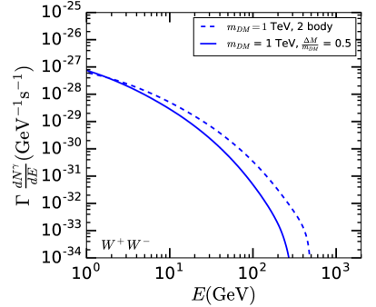
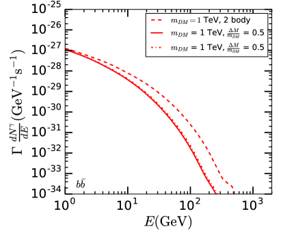
Figure 1: Left panel: $\gamma$-ray spectrum ($\Gamma\frac{dN^{\gamma}}{dE}$) for the decay processes $\phi\rightarrow W^{+}W^{-}$ (dashed curve) and $\phi_{2}\rightarrow\phi_{1}W^{+}W^{-}$ (solid curve). In the latter case, the (normalised) energy distribution of $W^{+}/W^{-}$ is governed by Eqn. LABEL:eqn:diboson_dist. Right panel: $\gamma$-ray spectrum for the decay processes $\phi\rightarrow b\bar{b}$ (dashed curve) and $\phi_{2}\rightarrow\phi_{1}b\bar{b}$ (solid and dashed-dotted curves). For three-body decays the (normalised) energy distributions of $b/\bar{b}$ is governed by Eqns. B.7 (solid line) and B.8 (dashed-dotted line). Here $m_{DM}=1$ TeV ($\frac{\Delta M}{m_{DM}}$ = 0.5 for multicomponent scenario) and $\Gamma=10^{-28}s^{-1}$.

The galactic contribution to the total $\gamma$-ray flux in eqn 3.8 has been calculated following [11] by taking the entire high-latitude sky (i.e. $0^{\degree}<|l|<180^{\degree}$) for $|b|>20^{\degree}$ into account. Note that this galactic contribution is not truly isotropic and can vary by a factor of 5 within the range of angles considered. However, this variation is less than $10\%$ within $45^{\degree}$ of the anti-galactic center (i.e $180^{\degree}-45^{\degree}<l<180^{\degree}+45^{\degree}$). Hence, if one takes the contribution towards anti-galactic center only (see [60, 61]), the galactic $\gamma$-ray flux can be treated more or less isotropic. In this case the total $\gamma$-ray flux can decrease at most by a factor of 5 than the flux predicted here and thus the limits on the dark matter decay width (presented in sec.4) will also be weakened at most by the same factor. Since the decay width is proportional to the square of the Wilson coefficients, the corresponding limits on these coefficients will be relaxed maximally by a factor of $\sim 2.2$. This will widen the available DM parameter space that can be probed by future radio telescopes like SKA.

We have shown for illustration the $\gamma$-ray distributions ($\Gamma\frac{dN^{\gamma}}{dE_{\gamma}}$) originating from the decays $\phi\rightarrow\,W^{+}W^{-}$ ($\phi\rightarrow b\bar{b}$) and $\phi_{2}\rightarrow\phi_{1}W^{+}W^{-}$ ($\phi_{2}\rightarrow\phi_{1}b\bar{b}$) in the left (right) panel of Fig 1 for a benchmark value of $m_{DM}$, $\Gamma$ and $\Delta\,M/m_{DM}$. Clearly for the three-body decays a substantial energy is taken away by $\phi_{1}$, thereby softening the corresponding $\gamma$-ray spectrum.

3.2 DM induced radio flux

The SM products of DM decay inside a dSph generate $e^{\pm}$ pairs through cascade decays, whose abundance is decided by the source function ($Q_{e}(E,r)$) [9]:

$$Q_{e}(E,r)=\Gamma\times\sum_{f}\frac{dN^{e}_{f}}{dE}(E)B_{f}\times\frac{\rho_{d}(r)}{m_{DM}}.$$ (3.9)

where $dN^{e}_{f}/dE$ is the differential distribution of the $e^{\pm}$ produced per decay in the final state $f$ with branching ratio $B_{f}$. The differential distribution is obtained using [51, 52]. $\rho_{d}(r)$ is the DM density profile of a dSph as a function of radial distance $r$ from the centre of the dSph. As already mentioned, we have taken the dSph Draco assuming a NFW profile as given in Eqn. 3.3 with $\rho_{0}=1.4$ GeV. cm^-3 and $r_{s}=1.0$ kpc [62]. We have used Draco for predicting the radio signal as various relevant parameters like the J-factor are somewhat better constrained for this dSph [65]. However, these parameters are also well-measured for other dSph’s such as Seg1, Carina, Fornax, Sculptor etc [65, 66, 67]. Draco is used for illustration in our analysis.

The produced electron(positron) diffuses through the galactic medium and loses energy via several processes like Inverse-Compton scatterings(IC), Synchroton radiation(Synch), Coulomb effect, bremsstrahlung etc. The final $e^{\pm}$ distribution $\frac{dn_{e}}{dE}(E,r)$ is obtained by solving the differential equation [68, 62, 69],

$$D(E)\nabla^{2}\left(\frac{dn_{e}}{dE}\right)+\frac{\partial}{\partial E}\left(b(E)\frac{dn_{e}}{dE}\right)+Q_{e}(E,r)=0$$ (3.10)

where the diffusion parameter $D(E)$ has been parametrized as $D(E)=D_{0}\,(\dfrac{E}{\rm GeV})^{0.3}$. The radius of the diffusion zone is assumed to be $2.5$ kpc [62]. The energy loss coefficient $b(E)$ can be expressed as

$$b(E) = b^{0}_{IC}\left(\frac{E}{\rm GeV}\right)^{2}+b^{0}_{Synch}\left(\frac{E}{\rm GeV}\right)^{2}\left(\frac{B}{\mu G}\right)^{2}$$ (3.11)

$$+b^{0}_{Coul}n_{e}\left[1+\frac{\log\left(\frac{E/m_{e}}{n_{e}}\right)}{75}\right]+b^{0}_{Brem}n_{e}\left[\log\left(\frac{E/m_{e}}{n_{e}}\right)+0.36\right],$$

where the values of the energy loss coefficients are $b^{0}_{IC}\simeq 0.25$, $b^{0}_{Synch}\simeq 0.0254$, $b^{0}_{Coul}\simeq 6.13$ $b^{0}_{Brem}\simeq 1.51$, all in units of $10^{-16}$ GeV s^-1. $m_{e}$ denotes the electron mass and $n_{e}$ is the average thermal electron density (value of $n_{e}\approx 10^{-6}$ inside a dSph) [68, 69].

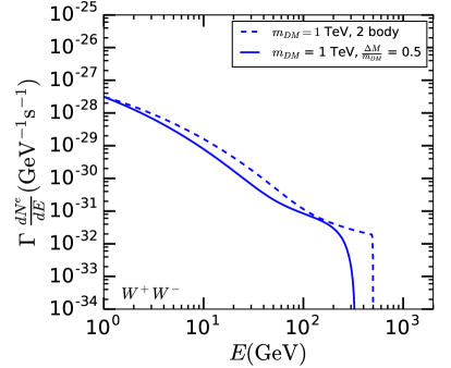
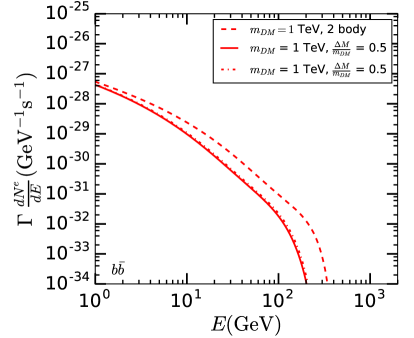
Figure 2: Left panel: $e^{\pm}$ spectrum ($\Gamma\frac{dN^{e}}{dE}$) for the decay processes $\phi\rightarrow W^{+}W^{-}$ (dashed curve) and $\phi_{2}\rightarrow\phi_{1}W^{+}W^{-}$ (solid curve). In the later case, the (normalised) energy distribution of $W^{+}/W^{-}$ is governed by Eqn. LABEL:eqn:diboson_dist. Right panel: $e^{\pm}$ spectrum for the decay processes $\phi\rightarrow b\bar{b}$ (dashed curve) and $\phi_{2}\rightarrow\phi_{1}b\bar{b}$ (solid and dashed-dotted curves). For three-body decays the (normalised) energy distributions of $b/\bar{b}$ is governed by Eqns. B.7 (solid line) and B.8 (dashed-dotted line). Here $m_{DM}=1$ TeV ($\frac{\Delta M}{m_{DM}}$ = 0.5 for multicomponent scenario) and $\Gamma=10^{-28}s^{-1}$.

The final radio flux ($S_{\nu}$) as a function of frequency ($\nu$) is obtained by folding this $\frac{dn_{e}}{dE}$ with synchrotron power spectrum ($P_{Synch}(\nu,E,B)$) [32, 68, 62, 69] and integrating over the size of the emission region of the dSph ($\Delta\Omega$):

$$S_{\nu}(\nu)=\frac{1}{4\pi}\int_{\Delta\Omega}\,d\Omega\int_{l.o.s}\,ds\left(2\overset{m_{DM}/2}{\underset{m_{e}}{\int}}dE\frac{dn_{e}}{dE}(r(s,\Omega),E)P_{Synch}(\nu,E,B)\right).$$ (3.12)

As an example we have shown the $e^{\pm}$ distribution ($\Gamma\frac{dN^{e}}{dE}$) produced in the decays $\phi\rightarrow\,W^{+}W^{-}$ ($\phi\rightarrow b\bar{b}$) and $\phi_{2}\rightarrow\phi_{1}W^{+}W^{-}$ ($\phi_{2}\rightarrow\phi_{1}b\bar{b}$) in the left (right) panel of Fig. 2 for a benchmark value of $m_{DM}$, $\Gamma$, $\Delta\,M/m_{DM}$. The energy distributions are softer for three-body decays, as in the case of $\gamma$-rays. Fig. 3 encapsulates the resulting synchrotron fluxes ($S_{\nu}(\nu)$) where the values of the diffusion coefficient($D_{0}$) and magnetic field($B$) have been chosen to be $D_{0}=3\times 10^{28}\mbox{cm}^{2}\mbox{s}^{-1}$ and $B=1$ $\mu G$, for illustration [70, 62].

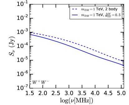
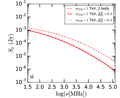
Figure 3: Left panel: Radio synchrotron flux, $S_{\nu}(\nu)$ (in Jy) for the decay processes $\phi\rightarrow W^{+}W^{-}$ (dashed curve) and $\phi_{2}\rightarrow\phi_{1}W^{+}W^{-}$ (solid curve). In the later case, the (normalised) energy distribution of $W^{+}/W^{-}$ is governed by Eqn. LABEL:eqn:diboson_dist. Right panel: Synchrotron flux for the decay processes $\phi\rightarrow b\bar{b}$ (dashed curve) and $\phi_{2}\rightarrow\phi_{1}b\bar{b}$ (solid and dashed-dotted curves). For three-body decays the (normalised) energy distributions of $b/\bar{b}$ is governed by Eqns. B.7 (solid line) and B.8 (dashed-dotted line). Here $m_{DM}=1$ TeV ($\frac{\Delta M}{m_{DM}}$ = 0.5 for multicomponent scenario) and $\Gamma=10^{-28}s^{-1}$. Choices of the astrophysical parameters are $D_{0}=3\times 10^{28}\mbox{cm}^{2}\mbox{s}^{-1}$ and $B=1$ $\mu G$.

4 Results

Using Fermi-LAT observation of isotropic gamma-ray background (IGRB) [16] we start by showing illustrative upper limits on the DM decay width $\Gamma$, considering only a single decay channel at a time (i) for a given dark matter mass ($m_{DM}$) in case of two-body decays of DM itself and (ii) for a chosen dark matter mass ($m_{DM}$) and two fixed values of $\Delta M/m_{DM}$, namely 0.9 (‘hierarchical scenario’) and 0.1 (‘degenerate scenario’) in case of three-body decays occurring within a multicomponent scalar dark sector. We have subsequently presented the upper limits on the Wilson coefficients in Eqns. 2.3 and 2.5 considering only one effective operator at a time. This is a reasonable assumption since each operator presented is independently gauge invariant. We have thus taken into account in the ultimate analysis all the decay channels opened up by a particular operator. The upper limits have been determined following the procedure of [11].

In each of the above cases we have also presented the sensitivity reach of the upcoming Square Kilometre Array (SKA). A large effective area and better baseline coverage help the SKA to achieve a significantly higher surface brightness sensitivity compared to existing radio telescopes. We have used the documents provided in the SKA website [31] for estimating the noise sensitivity. The higher sensitivity allows one to observe very low intensity radio signal coming from ultra-faint dSph’s which are estimated to have sizable DM densities, and the radio synchrotron signals from them possibly have less astrophysical background, since they have low rates of star formation. For details of the analysis see reference [32].

To present our results for SKA we have assumed some benchmark values of the diffusion coefficient and the magnetic field, namely, $D_{0}=3\times 10^{28}\mbox{cm}^{2}\mbox{s}^{-1}$ and $B=1$ $\mu G$. However, these astrophysical parameters are not very well constrained yet for a dSph [71, 10]. Though the proximity to our galaxy suggests that $B\approx 1$ $\mu G$ is a reasonable possibility [71], similar guidelines regarding $D_{0}$ hardly exists. Keeping this in mind, we have also shown the allowed astrophysical parameter space ($B-D_{0}$ plane) that can give rise to visible signal at SKA when the particle physics parameters are set at benchmark values consistent with IGRB observation.

4.1 Limits on particle physics parameters

4.1.1 Decay to Gauge bosons

Fig. 4 shows the upper limits on the DM decay widths ($\Gamma$) from Fermi-LAT observations as well as the sensitivity reach of the SKA in the channels $W^{+}W^{-}$(upper panel, left), $ZZ$(upper panel, right), $Z\gamma$(lower panel, left) and $\gamma\gamma$ (lower panel, right). We have assumed 100% branching ratio to each of these decay modes. It is important to point out that the decays of DM (or dark sector particles) to $Z\gamma$ and $\gamma\gamma$ are associated with primary (direct) photons. Since Fermi-LAT is mostly sensitive to photons in the energy range a few MeV-1 TeV and the direct photons produced in the $Z\gamma$ and $\gamma\gamma$ final states for $m_{DM}>1\,$TeV fall outside the energy range of Fermi-LAT, the corresponding limits weakens [16]. The future generation gamma-ray experiment like CTA [22, 23] can improve over Fermi-LAT in this range of parameters. We have adopted the strategy outlined in [36] to calculate sensitivity reach of CTA in the channels $Z\gamma$ and $\gamma\gamma$, which will show up as sharp spectral features on top of otherwise isotropic background flux of electrons+gamma-rays. The sensitivity reach of SKA in each of the cases have been shown which is nearly 4 to 2 orders of magnitude stronger depending on the DM mass $m_{DM}$ barring the $\gamma\gamma$ final state. In case of the $\gamma\gamma$ final state the primary (off-shell) photons can split into $e^{+}e^{-}$ pairs or other SM particle pairs which subsequently generate SKA-detectable radio signal . Since this splitting is suppressed by $\alpha_{\rm EM}$, the SKA sensitivity can be stronger by 2 to 1 order of magnitude only (see fig. 4 bottom panel, right). Better sensitivity of SKA is mostly attributed to its large cross-sectional area and low threshold [31]. Of course, it also depends on the choice of astrophysical parameters ($B,D_{0}$). In our case we have assumed that $D_{0}=3\times 10^{28}\mbox{cm}^{2}\mbox{s}^{-1}$ and $B=1$ $\mu G$ which are reasonable choices for dSph such as Draco. A more conservative choice, i.e, a larger $D_{0}$ or a lower $B$ will raise the sensitivity level.

The limits and sensitivities for the two-body decays $\phi\rightarrow VV^{\prime}$ is the strongest one since the final state $VV^{\prime}$ has the energy $m_{DM}$ available to them in these cases. For the three-body decays $\phi_{2}\rightarrow\phi_{1}VV^{\prime}$, on the other hand, even if one neglects the energy carried away by $\phi_{1}$ the energy available to $VV^{\prime}$ is $\approx\Delta M<m_{DM}$. Thus the energy distribution of the final state photons or $e^{\pm}$ softens for the three-body decays(see Fig.1 and 2). This explains why the limits weakens for three-body decays as compared to two-body decays and also by at least an order of magnitude in case of $\Delta M/m_{DM}=0.1$ compared to $\Delta M/m_{DM}=0.9$. The (normalised) energy distribution of $V/V^{\prime}$, produced in the decay $\phi_{2}\rightarrow\phi_{1}VV^{\prime}$, is governed by the Eqn. LABEL:eqn:diboson_dist.

In Fig. 5 we have shown the constraints obtained from Fermi-LAT and the sensitivity reach expected from SKA for gauge invariant wilson coefficients $f_{WW}$, $f_{BB}$ considering $\Lambda=10^{16}$ GeV for illustration. The operator proportional to $f_{WW}$ opens up all the channels $W^{+}W^{-},ZZ,Z\gamma,\gamma\gamma$ while $f_{BB}$ opens up $ZZ,Z\gamma,\gamma\gamma$ (see Eqns. A.3 and B.3). Thus in order to calculate limits on those parameters one needs to consider contribution from all the channels with appropriate branching fractions. As mentioned earlier, for channels such as $Z\gamma$ and $\gamma\gamma$ (which have direct photon(s) in their final states), both Fermi-LAT limit (mainly for lower DM mass) and CTA limit (mainly for higher DM mass) have been used. One should note that $\gamma\gamma$ channel has a branching ratio proportional to $\cos^{4}\theta_{W}$ when $f_{BB}$ is open compared to the $\sin^{4}\theta_{W}$ dependence, when $f_{WW}$ is open and thus the limit on $f_{BB}$ is affected more by the inclusion of the sensitivity reach of CTA. This understanding is reflected in the kink around the energy, beyond which CTA offers a better probe for direct photons than Fermi-LAT. We have also shown the limits on the wilson coefficient $f_{B}$. The operator proportional to $f_{B}$ gives only a two-body decay $\phi_{2}\rightarrow\phi_{1}Z$ (see the discussions regarding Eqn. B.4).

4.1.2 Decay to Fermions

In Fig. 6 we have shown the upper limits (for Fermi-LAT) and sensitivity (for SKA) on the decay width ($\Gamma$) as a function of $m_{DM}$ assuming the decay occurs dominantly through $b\bar{b}$ (upper panel, left), $t\bar{t}$ (upper panel, right) and $\tau^{+}\tau^{-}$ (lower panel). The (normalised) energy distribution of a fermion($f$)/anti-fermion($\bar{f}$) produced in the three-body decay $\phi_{2}\rightarrow\phi_{1}f\bar{f}$ is considered to be the one governed by Eqn. B.7. One can check that the other energy distribution provided in Eqn. B.8 produces almost similar limits (and sensitivity) for any of the aforementioned fermionic channels, as expected from Figs. 1 and 2.

In Fig. 7 we have shown the constrains obtained from Fermi-LAT and the sensitivity reach expected from SKA on the wilson coefficient $f_{qq}$ in case of the two-body decay of DM itself (upper left panel) and in case of decays in the dark sector (lower left panel). Here $f_{qq}$ is the coupling to the quarks arising from $\mathcal{L}^{\rm fermion,1}_{dim-5}$ in Eqn. 2.3 and $\mathcal{L}^{\rm fermion,1}_{dim-6}$ 2.5. For simplicity we have assumed that both the left and right handed quarks have the same values of this coupling. Also, we have considered that $f_{qq}\neq 0$ only for third generation of quarks which via gauge invariance dictates the relative contribution of the channels $b\bar{b}$ and $t\bar{t}$. It is quite evident that the limits from SKA on $f_{qq}$ will be stronger than Fermi-LAT by more than one order of magnitude up to $m_{DM}\simeq 100\,$TeV .

The upper right and lower right panel of the same figure shows the constraints on the wilson coefficient $f_{ll}$ in case of the two-body decay of DM itself and in case of decays in the dark sector, respectively. Here also, we have assumed that both the left and right handed leptons have the same values of this coupling which appears only for the third generation of leptons. The only visible decay products as a result of switching on $f_{ll}$ being $\tau^{+}\tau^{-}$ the limits on $f_{ll}$ is straightforward to obtain from the decay widths themselves. Although the sensitivity of SKA to $\tau^{+}\tau^{-}$ final states decreases rapidly as the $m_{DM}$ increases (see the lower panel of Fig.6), SKA can still probe larger parameter space compared to Fermi-LAT even up to $m_{DM}\simeq 100\,\,$TeV.

Fig. 8 shows the constrains obtained from Fermi-LAT and the sensitivity reach expected from SKA on the wilson coefficients $f_{bbH}$, $f_{ttH}$ and $f_{llH}$ in case of the two-body decay of DM itself (left column) and in case of decays in the dark sector (right column). Here $f_{bbH}$, $f_{ttH}$ and $f_{llH}$ are the couplings to the $b$ and $t$ quarks and $\tau$ lepton following from $\mathcal{L}^{\rm fermion,2}_{dim-5}$ in Eqn. 2.3 and $\mathcal{L}^{\rm fermion,2}_{dim-6}$ in Eqn. 2.5. For simplicity, we have considered the couplings to be non-zero only for the third generation of fermions. It is clear that the limits expected from 500 hours of observation at SKA on $f_{bbH}$ and $f_{ttH}$ will be stronger than Fermi-LAT by more than one order of magnitude up to $m_{DM}\simeq 100\,$TeV. Although the sensitivity of SKA to the $\tau^{+}\tau^{-}$ channel decreases rapidly as $m_{DM}$ increases (see the lower panel of Fig. 6), SKA can still probe larger parameter space compared to Fermi-LAT even up to $m_{DM}\simeq 100\,\,$TeV.

4.2 Limits on Astrophysical parameters

As of now we have shown the particle physics parameter space that can be probed using SKA choosing a benchmark values of $D_{0}=3\times 10^{28}\mbox{cm}^{2}\mbox{s}^{-1}$ and $B=1$ $\mu G$. Here we have shown which region of the astrophysical parameters $B-D_{0}$ will produce a observable DM decay signal at SKA assuming a set of particle physics parameters that has not been ruled out by isotropic $\gamma$-ray background (IGRB) observation.

In Fig. 9 we have considered either only $f_{WW}$ is non-zero (left panel) or only $f_{BB}$ is non-zero (right panel) and chosen a benchmark value $m_{DM}=10\,$TeV while the values of the wilson coefficients are dictated by the corresponding upper limits as obtained from Fermi-LAT (and in case of $Z\gamma$ and $\gamma\gamma$ channels by CTA) as shown in Fig. 5. The regions above the curves shown in the figures are favourable for observation in SKA (assuming a 500 hours of observation). The corresponding limits on $B-D_{0}$ for $f_{B}\neq 0$ can be obtained similarly. The results for $f_{qq}$ (Fig. 10, left panel) , $f_{ll}$ (Fig. 10, right panel) as well as $f_{bbH}$ (Fig. 11, left panel) and $f_{llH}$ (Fig. 11, right panel) should also be interpreted in the same way. Note that if one considers only the anti-galactic contribution to the galactic $\gamma$-ray flux in deriving the $\gamma$-ray constraints on the Wilson coefficients (as discussed in sec. 3.1), the limits on the $B-D_{0}$ plane presented here can become stronger at most by a factor of 5.

Our general conclusion emerges from Figs. 9-11. We demonstrate that the SKA can do considerably better than $\gamma$-ray observations for the range of $m_{\rm DM}$ under focus here. If SKA indeed records such radio signals as predicted here, then, some independent information on $m_{\rm DM}$ and $\Gamma$ may enable one to identify regions in the $B-D_{0}$ plane, which are consistent with the DM decay observations. Similar conclusions involving DM annihilations in a dSph can be found in [32].

5 Conclusion

We have carried out a study of long-lived DM with its decay showing up in $\gamma$-ray as well as radio telescope observations. In order to comply with constraints on DM lifetime, the decay interactions have been parametrised by higher-dimensional operators. Both two-body decays of a scalar DM particle and three-body decays of quasi-stable particles within a dark sector have been considered, the SM particles among decay products being pairs of gauge bosons as well as fermions of the third family.

Constraints on the coefficients of the various operators have been obtained from existing $\gamma$-ray observations. The Fermi-LAT results are found to be most constraining in this respect, In comparison, the proposed CTA observations are found to yield weaker constraints, except in cases where at least one $\gamma$-ray photon is directly produced in decay, as opposed to photons coming via cascades.

However, radio synchrotron signals from dSph’s are found to provide better probes into DM decays, by enabling exploration of regions which cannot be ruled out by either the Fermi-LAT data or the CTA. This is true even for DM masses well-above a TeV. Using as benchmark 500 hours of observation at the upcoming SKA radio telescope, we find such a conclusion to hold for DM masses ranging up to tens of TeV.

It is also shown how some independent conclusion on DM mass and its decay rate can enable one to identify viable regions of astrophysical parameters pertaining to a dSph under observation. In this spirit, we demonstrate how to find allowed ranges in the space spanned by the diffusion coefficient in the dSph and the galactic magnetic field, for sample values of the DM particle mass and its decay rate, consistent with $\gamma$-ray observation.

6 Acknowledgements

The authors thank Alejandro Ibarra, Saurav Mitra, Tirthankar Roy Choudhury and Steven Tingay for their help in learning about gamma-ray and radio signals of dark matter. AG and AK acknowledges the hospitality of the Theoretical Physics Department, Indian Association for Cultivation of Science(IACS), Kolkata and Indian Institute of Science Education and Research(IISER), Kolkata where a substantial part of the project was carried out. This work was partially supported by funding available from the Department of Atomic Energy, Government of India, for the Regional Centre for Accelerator-based Particle Physics (RECAPP), Harish-Chandra Research Institute, Allahabad.

Appendix A Single-component dark matter

A.1 Decay to gauge bosons

The decay $\phi\rightarrow\,V\,V^{\prime}$ is governed by the term

$$\dfrac{f_{VV^{\prime}}}{\Lambda}\phi\,V_{\mu\nu}V^{\prime\mu\nu}$$ (A.1)

and the partial width is,

$$\Gamma_{VV^{\prime}} = \frac{1}{2\pi}\left(\frac{f_{VV^{\prime}}}{\Lambda}\right)^{2}\,M^{3}\sqrt{1-\frac{2(m^{2}_{V}+m^{2}_{V^{\prime}})}{M^{2}}+\frac{(m^{2}_{V}-m^{2}_{V^{\prime}})^{2}}{M^{4}}}$$ (A.2)

$$\left[1-\frac{2(m^{2}_{V}+m^{2}_{V^{\prime}})}{M^{2}}+\frac{(m^{4}_{V}+m^{4}_{V^{\prime}}+4m^{2}_{V}m^{2}_{V^{\prime}})}{M^{4}}\right].$$

Here,

$$f_{VV^{\prime}}=\begin{cases}\displaystyle{f_{WW}}&~{}~{}{\rm for}\,V=W^{+},V^{\prime}=W^{-}\\ \displaystyle{\frac{1}{\sqrt{2}}\left(\cos^{2}\theta_{W}f_{WW}+\sin^{2}\theta_{W}f_{BB}\right)}&~{}~{}{\rm for}\,V=Z,V^{\prime}=Z\\ \displaystyle{\cos\theta_{W}\sin\theta_{W}\left(f_{WW}-f_{BB}\right)}&~{}~{}{\rm for}\,V=Z,V^{\prime}=\gamma\\ \displaystyle{\frac{1}{\sqrt{2}}\left(\sin^{2}\theta_{W}f_{WW}+\cos^{2}\theta_{W}f_{BB}\right)}&~{}~{}{\rm for}\,V=\gamma,V^{\prime}=\gamma\end{cases}\;.$$ (A.3)

A.2 Decay to fermions

The decay of $\phi$ to fermion pairs is parametrized as,

$$\frac{f_{ff}}{\Lambda}\phi\,\left(\bar{f}_{L}\gamma^{\mu}{\partial}_{\mu}f_{L}+\bar{f}_{R}\gamma^{\mu}{\partial}_{\mu}f_{R}\right)+\frac{f_{ffH}}{\Lambda}\phi\left[\bar{f}_{L}f_{R}H+h.c\right]$$ (A.4)

The decay width from the first term in Eqn. A.4,

$$\Gamma_{f\bar{f}} = \,N_{c}\,\frac{1}{8\pi}\left(\frac{f_{ff}}{\Lambda}\right)^{2}\,m^{2}_{f}\,M\,\left(1-\frac{4m^{2}_{f}}{M^{2}}\right)^{3/2}.$$ (A.5)

and from the second term in Eqn. A.4,

$$\Gamma_{f\bar{f}} = \,N_{c}\,\frac{1}{16\pi}\left(\frac{f_{ffH}}{\Lambda}\right)^{2}\,v^{2}\,M\,\left(1-\frac{4m^{2}_{f}}{M^{2}}\right)^{3/2}.$$ (A.6)

where $N_{c}=3$ for quarks and $N_{c}=1$ for leptons.

Appendix B Multicomponent dark sector

B.1 Decay to gauge bosons

1. The decay $\phi_{2}\rightarrow\,\phi_{1}\,V\,V^{\prime}$ is governed by

   $$\dfrac{f_{VV^{\prime}}}{\Lambda^{2}}\phi_{2}\phi_{1}V_{\mu\nu}V^{\prime\mu\nu}$$ (B.1)

   The energy distribution of the vector boson $V$ originating from $\phi_{2}\rightarrow\phi_{1}\!VV^{\prime}$ is,

   $$\frac{d\Gamma_{\phi_{1}\,VV^{\prime}}}{dx_{v}}\, = \,\left(\frac{f_{VV^{\prime}}}{\Lambda^{2}}\right)^{2}\,\frac{M^{5}_{2}}{32\pi^{3}}\sqrt{x^{2}_{v}-4r^{2}_{v}}\,\lambda^{1/2}\left(\sqrt{1+r^{2}_{v}-x_{v}}\,,\,r_{1},\,r_{v^{\prime}}\right)$$

   $$\bigg{[}2r^{2}_{v}r^{2}_{v^{\prime}}+\frac{1}{12}\bigg{\{}3\frac{(x_{v}-2r^{2}_{v})^{2}}{(1+r^{2}_{v}-x_{v})^{2}}(1-r^{2}_{1}+r^{2}_{v}+r^{2}_{v^{\prime}}-x_{v})^{2}$$

   $$\,+(x^{2}_{v}-4r^{2}_{v})\lambda\left(\sqrt{1+r^{2}_{v}-x_{v}}\,,\,r_{1},\,r_{v^{\prime}}\right)\bigg{\}}\bigg{]}$$

   where $r_{v(v^{\prime})}=\dfrac{m_{v(v^{\prime})}}{M_{2}}\,,\,r_{1}=\dfrac{M_{1}}{M_{2}}\,,\,x_{v}=\dfrac{2E_{v}}{M_{2}}$ and $2\,r_{v}\,\leq\,x_{v}\,\leq\,\left(1-r^{2}_{1}+r^{2}_{v}-r^{2}_{v^{\prime}}-2r_{1}r_{v^{\prime}}\right)$.
   The kallen-lambda function is given by, $\lambda\left(a,b,c\right)\,=\,\left(1-\dfrac{2\left(b^{2}+c^{2}\right)}{a^{2}}+\dfrac{\left(b^{2}-c^{2}\right)^{2}}{a^{4}}\right)$.
   

   Here,

   $$f_{VV^{\prime}}=\begin{cases}\displaystyle{f_{WW}}&~{}~{}{\rm for}\,V=W^{+},V^{\prime}=W^{-}\\ \displaystyle{\frac{1}{\sqrt{2}}\left(\cos^{2}\theta_{W}f_{WW}+\sin^{2}\theta_{W}f_{BB}\right)}&~{}~{}{\rm for}\,V=Z,V^{\prime}=Z\\ \displaystyle{\cos\theta_{W}\sin\theta_{W}\left(f_{WW}-f_{BB}\right)}&~{}~{}{\rm for}\,V=Z,V^{\prime}=\gamma\\ \displaystyle{\frac{1}{\sqrt{2}}\left(\sin^{2}\theta_{W}f_{WW}+\cos^{2}\theta_{W}f_{BB}\right)}&~{}~{}{\rm for}\,V=\gamma,V^{\prime}=\gamma\end{cases}\;.$$ (B.3)

2. Due to angular momentum conservation the decay $\phi_{2}\rightarrow\phi_{1}\gamma$ is forbidden and the operator

   $$\dfrac{f_{B}}{\Lambda^{2}}\left(\partial_{\mu}\phi_{2}\partial_{\nu}\phi_{1}-\partial_{\nu}\phi_{2}\partial_{\mu}\phi_{1}\right)B_{\mu\nu}$$ (B.4)

   can only trigger the decay $\phi_{2}\rightarrow\phi_{1}Z$ .

   The emitted $Z$-boson has a fixed energy $E_{z}=M_{2}/2\left(1-r^{2}_{1}+r^{2}_{z}\right)$ and the corresponding width is,

   $$\Gamma_{\phi_{1}Z}=\left(\frac{f_{B}}{\Lambda^{2}}\right)^{2}M^{3}_{2}\frac{\sin^{2}\theta_{W}m^{2}_{z}}{16\pi}\lambda^{3/2}\left(1,r_{1},r_{z}\right)$$ (B.5)

B.2 Decay to fermions

The interactions are,

$$\frac{f_{ff}}{\Lambda^{2}}\phi_{2}\overset{\leftrightarrow}{\partial}_{\mu}\phi_{1}\,\bar{f}\gamma^{\mu}\,f+\frac{f_{ffH}}{\Lambda^{2}}\frac{v}{\sqrt{2}}\phi_{2}\phi_{1}\,\bar{f}\,f$$ (B.6)

For simplicity in our analysis we have taken only one operator at a time.

1. The differential distribution of the fermion due to first term of Eqn. B.6.

   $$\frac{d\Gamma_{\phi_{1}\!f\bar{f}}}{dx}\, = \,N_{c}\,\left(\frac{f_{ff}}{\Lambda^{2}}\right)^{2}\,\frac{M^{5}_{2}}{16\,\pi^{3}}\bigg{[}\sqrt{x^{2}-4\,r^{2}_{f}}\,\lambda^{1/2}\left(\sqrt{1+r^{2}_{f}-x},r_{1},r_{f}\right)$$ (B.7)

   $$\frac{2(1-r^{2}_{1}-x)(1+r^{2}_{f}-x)-(1-x)(2-x)(1-r^{2}_{1}+2r^{2}_{f}-x)}{\left(1+r^{2}_{f}-x\right)}\bigg{]}$$

   where $r_{f}=\dfrac{m_{f}}{M_{2}}$,$r_{1}=\dfrac{M_{1}}{M_{2}}$ and $x=\dfrac{2E_{f}}{M_{2}}$ with $2r_{f}\leq\!x\leq\!\left(1-r^{2}_{1}-2r_{1}r_{f}\right)$.
   

2. The differential energy distribution of the fermions for the second operator in Eqn. B.6 is,

   $$\frac{d\Gamma_{\phi_{1}\!f\bar{f}}}{dx}\, = \,N_{c}\,\left(\frac{f_{ffH}}{\Lambda^{2}}\right)^{2}\,\frac{v^{2}M^{3}_{2}}{512\pi^{3}}\bigg{[}\sqrt{x^{2}-4\,r^{2}_{f}}\,\lambda^{1/2}\left(\sqrt{1+r^{2}_{f}-x},r_{1},r_{f}\right)$$ (B.8)

   $$\frac{x(1-r^{2}_{1}-x)+2r^{2}_{f}(-3+r^{2}_{1}+4x)-8r^{4}_{f}}{\left(1+r^{2}_{f}-x\right)}\bigg{]}$$

   where $r_{f}=\dfrac{m_{f}}{M_{2}}\,,\,r_{1}=\dfrac{M_{1}}{M_{2}}\,,\,x=\dfrac{2E_{f}}{M_{2}}$ and $2\,r_{f}\,\leq\,x\,\leq\,\left(1-r^{2}_{1}-2r_{1}r_{f}\right)$.
   

   Here $N_{c}=3$ for quarks and $N_{c}=1$ for leptons.

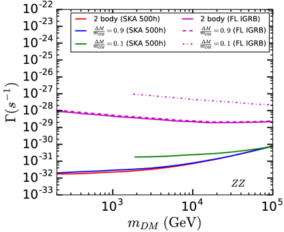
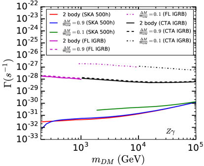
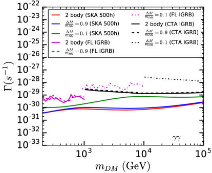
Figure 4: SKA sensitivity and the upper limit from $\gamma$-ray observation in the $\Gamma-m_{DM}$ plane for the decay of a DM (or a dark sector) particle of mass $m_{DM}$ to various vector boson final states ($VV^{\prime}$), i.e. either $W^{+}W^{-}$ (upper-left panel) or $ZZ$ (upper-right panel) or $Z\gamma$ (lower-left panel) or $\gamma\gamma$ (lower-right panel). The red, blue and green curves denote the required values of $\Gamma$ to detect the radio fluxes at SKA (assuming a 500 hours of observation) from Draco dSph for the processes $\phi\rightarrow VV^{\prime}$ and $\phi_{2}\rightarrow\phi_{1}VV^{\prime}$ (with $\frac{\Delta M}{m_{DM}}=0.9$ and 0.1), respectively. The (normalised) energy distribution of $V/V^{\prime}$ in three-body decay is governed by Eqn. LABEL:eqn:diboson_dist. The astrophysical parameters used are $D_{0}=3\times 10^{28}\mbox{cm}^{2}\mbox{s}^{-1}$ and $B=1$ $\mu G$. The solid, dashed and dashed-dotted magenta lines are the corresponding upper limits on $\Gamma$ from the observation of isotropic $\gamma$-ray background (IGRB) by Fermi-LAT (FL). In case of $Z\gamma$ and $\gamma\gamma$, along with Fermi-LAT, the projected sensitivity from the IGRB observation by CTA (black curves; assuming 500 hours of observation) also has been shown (see the text for details).

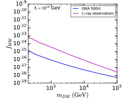
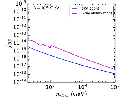
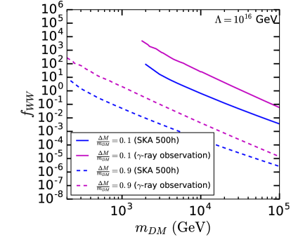
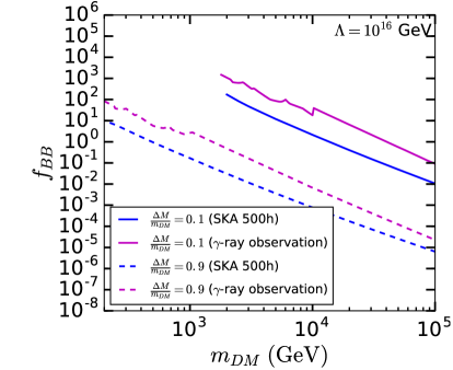
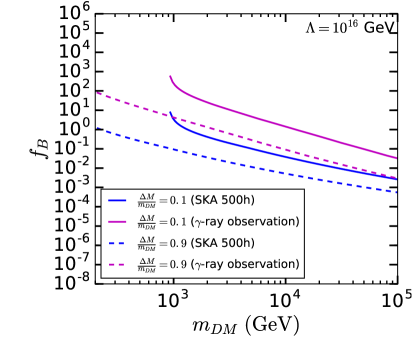
Figure 5: Upper panel: Sensitivity of SKA (blue lines; assuming a 500 hours of observation for Draco dSph) to various gauge boson effective couplings (listed in Eqn. 2.3) which governs the two-body decays of a DM particle of mass $m_{DM}$ to the pairs of gauge boson final states. The astrophysical parameters used are $D_{0}=3\times 10^{28}\mbox{cm}^{2}\mbox{s}^{-1}$ and $B=1$ $\mu G$. The magenta lines are the corresponding limits obtained from the isotropic $\gamma$-ray background (IGRB) observation. Middle and lower panels: Similar constraints on the gauge boson effective couplings (listed in Eqn. 2.5) which give rise to the three-body decays of a DM particle of mass $m_{DM}$. Two different values of $\Delta M/m_{DM}$ have been considered, $\Delta M/m_{DM}=0.1$ (solid lines) and 0.9 (dashed lines).

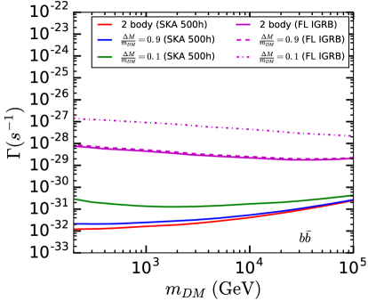
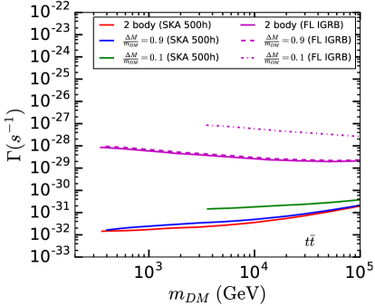
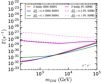
Figure 6: SKA sensitivity and the upper limit from $\gamma$-ray observation in the $\Gamma-m_{DM}$ plane for the decay of a DM (or a dark sector) particle of mass $m_{DM}$ to various fermionic final states ($f\bar{f}$), i.e. either $b\bar{b}$ (upper-left panel) or $t\bar{t}$ (upper-right panel) or $\tau^{+}\tau^{-}$ (lower panel). The red, blue and green curves denote the required values of $\Gamma$ to detect the radio fluxes from Draco dSph for the processes $\phi\rightarrow f\bar{f}$ and $\phi_{2}\rightarrow\phi_{1}f\bar{f}$ (with $\frac{\Delta M}{m_{DM}}=0.9$ and 0.1), respectively. The (normalised) energy distribution of $f/\bar{f}$ in three-body decay is governed by Eqn. B.7. The astrophysical parameters used are $D_{0}=3\times 10^{28}\mbox{cm}^{2}\mbox{s}^{-1}$ and $B=1$ $\mu G$. The solid, dashed and dashed-dotted magenta lines are the corresponding upper limits on $\Gamma$ from the observation of isotropic $\gamma$-ray background (IGRB) by Fermi-LAT (FL).

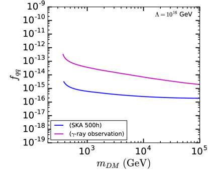
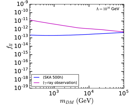
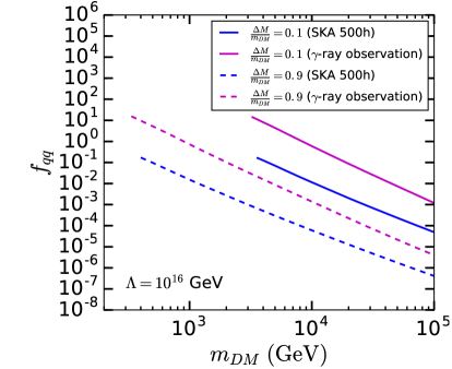
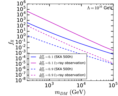
Figure 7: Upper panel: Sensitivity of SKA (blue lines; assuming a 500 hours observation for Draco dSph) to the effective couplings of $\mathcal{L}_{dim-5}^{\rm fermion,1}$, shown in Eqn. 2.3, which give the two-body decays of a DM particle of mass $m_{DM}$ to the pairs of fermions. $f_{qq}$ is the coupling to both $b$ and $t$ quarks and $f_{ll}$ is the coupling to $\tau$ lepton. The astrophysical parameters used are $D_{0}=3\times 10^{28}\mbox{cm}^{2}\mbox{s}^{-1}$ and $B=1$ $\mu G$. The magenta lines are the corresponding limits obtained from the isotropic $\gamma$-ray background (IGRB) observation. Lower panel: Similar constraints on the effective couplings of $\mathcal{L}_{dim-6}^{\rm fermion,1}$, shown in Eqn. 2.5, which give the three-body decays of a DM particle of mass $m_{DM}$. Two different values of $\Delta M/m_{DM}$ have been considered, $\Delta M/m_{DM}=0.1$ (solid lines) and 0.9 (dashed lines).

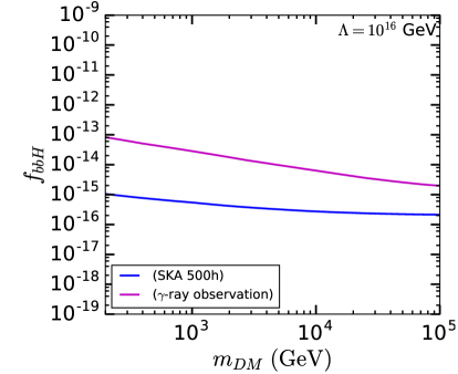
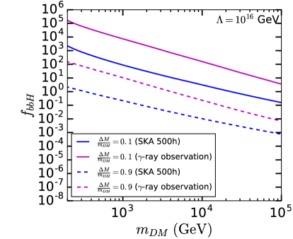
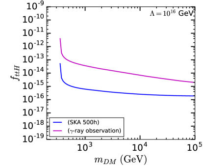
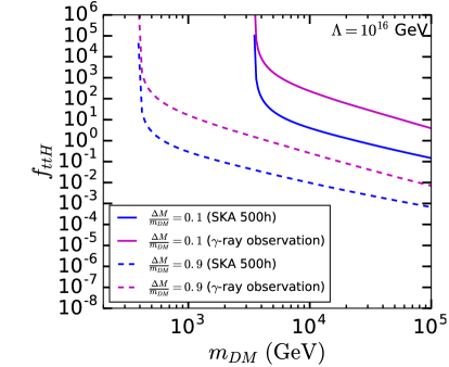
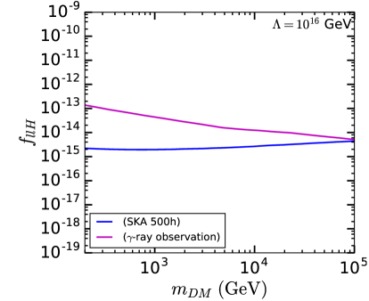
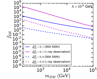
Figure 8: Left column: Sensitivity of SKA (blue lines; assuming a 500 hours observation for Draco dSph) to the effective couplings of $\mathcal{L}_{dim-5}^{\rm fermion,2}$, shown in Eqn. 2.3, which give rise to the two-body decays of a DM particle of mass $m_{DM}$ to a pair of fermions. $f_{bbH}$, $f_{ttH}$ and $f_{llH}$ are the couplings to $b$ quark, $t$ quark and $\tau$ lepton, respectively. The astrophysical parameters used are $D_{0}=3\times 10^{28}\mbox{cm}^{2}\mbox{s}^{-1}$ and $B=1$ $\mu G$. The magenta lines are the corresponding limits obtained from the isotropic $\gamma$-ray background (IGRB) observation. Right column: Similar constraints on the effective couplings of $\mathcal{L}_{dim-6}^{\rm fermion,2}$, shown in Eqn. 2.5, which causes the three-body decays of a DM particle of mass $m_{DM}$. Two different values of $\Delta M/m_{DM}$ have been considered, $\Delta M/m_{DM}=0.1$ (solid lines) and 0.9 (dashed lines).

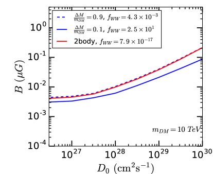
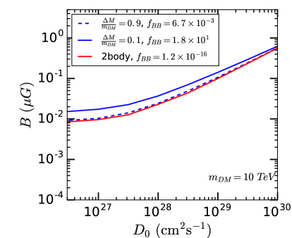
Figure 9: Limits in the $B-D_{0}$ plane to observe a DM decay induced radio signal at SKA (500 hours) from Draco dSph. It is assumed that the DM particle is of mass 10 TeV and it decays to various gauge boson final states through the gauge boson effective operators listed in Eqns. 2.3 and 2.5. The values of the effective couplings are kept fixed at the upper limits obtained from the isotropic $\gamma$-ray background (IGRB) at this DM mass (see Fig.5).

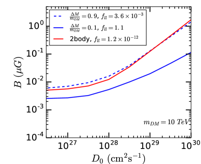
Figure 10: Limits in the $B-D_{0}$ plane to observe a DM decay induced radio signal at SKA (500 hours) from Draco dSph. It is assumed that the DM particle is of mass 10 TeV and it decays to various fermionic final states through the fermionic operators $\mathcal{L}^{\rm fermion,1}_{dim-5}$ and $\mathcal{L}^{\rm fermion,1}_{dim-6}$, listed in Eqns. 2.3 and 2.5, respectively. The values of the effective couplings are kept fixed at the upper limits obtained from the isotropic $\gamma$-ray background (IGRB) at this DM mass (see Fig.7).

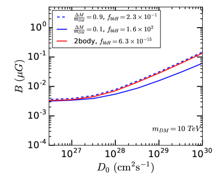
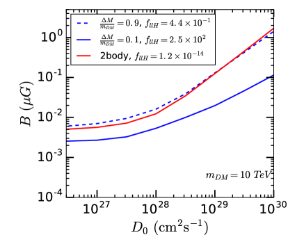
Figure 11: Limits in the $B-D_{0}$ plane to observe a DM decay induced radio signal at SKA (500 hours) from Draco dSph. It is assumed that the DM particle is of mass 10 TeV and it decays to various fermionic final states through the fermionic operators $\mathcal{L}^{\rm fermion,2}_{dim-5}$ and $\mathcal{L}^{\rm fermion,2}_{dim-6}$, listed in Eqns. 2.3 and 2.5, respectively. The values of the effective couplings are kept fixed at the upper limits obtained from the isotropic $\gamma$-ray background (IGRB) at this DM mass (see Fig.7).

References

- [1] XENON collaboration, E. Aprile et al., First Dark Matter Search Results from the XENON1T Experiment, Phys. Rev. Lett. 119 (2017) 181301, [1705.06655].
- [2] LUX Collaboration collaboration, D. S. Akerib et al., Limits on spin-dependent wimp-nucleon cross section obtained from the complete lux exposure, Phys. Rev. Lett. 118 (Jun, 2017) 251302.
- [3] L. Shchutska, Prospects for bsm searches at the high-luminosity lhc with the cms detector, Nuclear and Particle Physics Proceedings 273-275 (2016) 656 – 661.
- [4] Search for Supersymmetry at the high luminosity LHC with the ATLAS experiment, Tech. Rep. ATL-PHYS-PUB-2014-010, CERN, Geneva, Jul, 2014.
- [5] CMS Collaboration collaboration, Study of the Discovery Reach in Searches for Supersymmetry at CMS with 3000/fb, Tech. Rep. CMS-PAS-FTR-13-014, CERN, Geneva, 2013.
- [6] A. Cuoco, J. Heisig, M. Korsmeier and M. Krämer, Constraining heavy dark matter with cosmic-ray antiprotons, JCAP 1804 (2018) 004, [1711.05274].
- [7] Fermi-LAT collaboration, M. Ackermann et al., The Fermi Galactic Center GeV Excess and Implications for Dark Matter, Astrophys. J. 840 (2017) 43, [1704.03910].
- [8] Fermi-LAT, DES collaboration, A. Albert et al., Searching for Dark Matter Annihilation in Recently Discovered Milky Way Satellites with Fermi-LAT, Astrophys. J. 834 (2017) 110, [1611.03184].
- [9] M. Regis, L. Richter and S. Colafrancesco, Dark matter in the Reticulum II dSph: a radio search, JCAP 1707 (2017) 025, [1703.09921].
- [10] A. Natarajan, J. B. Peterson, T. C. Voytek, K. Spekkens, B. Mason, J. Aguirre et al., Bounds on Dark Matter Properties from Radio Observations of Ursa Major II using the Green Bank Telescope, Phys. Rev. D88 (2013) 083535, [1308.4979].
- [11] C. Blanco and D. Hooper, Constraints on Decaying Dark Matter from the Isotropic Gamma-Ray Background, JCAP 1903 (2019) 019, [1811.05988].
- [12] B.-Q. Lu and H.-S. Zong, Limits on dark matter from AMS-02 antiproton and positron fraction data, Phys. Rev. D 93 (2016) 103517, [1510.04032].
- [13] S. Ando and K. Ishiwata, Constraints on decaying dark matter from the extragalactic gamma-ray background, JCAP 1505 (2015) 024, [1502.02007].
- [14] R. Essig, E. Kuflik, S. D. McDermott, T. Volansky and K. M. Zurek, Constraining Light Dark Matter with Diffuse X-Ray and Gamma-Ray Observations, JHEP 11 (2013) 193, [1309.4091].
- [15] T. Cohen, K. Murase, N. L. Rodd, B. R. Safdi and Y. Soreq, γ -ray Constraints on Decaying Dark Matter and Implications for IceCube, Phys. Rev. Lett. 119 (2017) 021102, [1612.05638].
- [16] Fermi-LAT collaboration, M. Ackermann et al., The spectrum of isotropic diffuse gamma-ray emission between 100 MeV and 820 GeV, Astrophys. J. 799 (2015) 86, [1410.3696].
- [17] AMS collaboration, M. Aguilar et al., Precision Measurement of the Proton Flux in Primary Cosmic Rays from Rigidity 1 GV to 1.8 TV with the Alpha Magnetic Spectrometer on the International Space Station, Phys. Rev. Lett. 114 (2015) 171103.
- [18] AMS collaboration, M. Aguilar et al., Electron and Positron Fluxes in Primary Cosmic Rays Measured with the Alpha Magnetic Spectrometer on the International Space Station, Phys. Rev. Lett. 113 (2014) 121102.
- [19] H.E.S.S. collaboration, A. Abramowski et al., Diffuse Galactic gamma-ray emission with H.E.S.S, Phys. Rev. D90 (2014) 122007, [1411.7568].
- [20] H.E.S.S. collaboration, A. Abramowski et al., Search for dark matter annihilation signatures in H.E.S.S. observations of Dwarf Spheroidal Galaxies, Phys. Rev. D90 (2014) 112012, [1410.2589].
- [21] IceCube collaboration, M. G. Aartsen et al., Search for neutrinos from decaying dark matter with IceCube, Eur. Phys. J. C78 (2018) 831, [1804.03848].
- [22] CTA Consortium collaboration, M. Actis et al., Design concepts for the Cherenkov Telescope Array CTA: An advanced facility for ground-based high-energy gamma-ray astronomy, Exper. Astron. 32 (2011) 193–316, [1008.3703].
- [23] CTA Consortium collaboration, A. Morselli, The Dark Matter Programme of the Cherenkov Telescope Array, PoS ICRC2017 (2018) 921, [1709.01483].
- [24] H. Silverwood, C. Weniger, P. Scott and G. Bertone, A realistic assessment of the CTA sensitivity to dark matter annihilation, JCAP 1503 (2015) 055, [1408.4131].
- [25] V. Lefranc, E. Moulin, P. Panci and J. Silk, Prospects for Annihilating Dark Matter in the inner Galactic halo by the Cherenkov Telescope Array, Phys. Rev. D91 (2015) 122003, [1502.05064].
- [26] V. Lefranc, G. A. Mamon and P. Panci, Prospects for annihilating Dark Matter towards Milky Way’s dwarf galaxies by the Cherenkov Telescope Array, JCAP 1609 (2016) 021, [1605.02793].
- [27] N. Hiroshima, M. Hayashida and K. Kohri, Dependence of accessible dark matter annihilation cross-sections on the density profiles of dwarf spheroidal galaxies with the Cherenkov Telescope Array, Phys. Rev. D99 (2019) 123017, [1905.12940].
- [28] A. Viana, H. Schoorlemmer, A. Albert, V. de Souza, J. P. Harding and J. Hinton, Searching for Dark Matter in the Galactic Halo with a Wide Field of View TeV Gamma-ray Observatory in the Southern Hemisphere, JCAP 1912 (2019) 061, [1906.03353].
- [29] M. Pierre, J. M. Siegal-Gaskins and P. Scott, Sensitivity of CTA to dark matter signals from the Galactic Center, JCAP 1406 (2014) 024, [1401.7330].
- [30] K. Ishiwata, O. Macias, S. Ando and M. Arimoto, Probing heavy dark matter decays with multi-messenger astrophysical data, 1907.11671.
- [31] R. Braun et al. https://astronomers.skatelescope.org/wp-content/uploads/2017/10/SKA-TEL-SKO-0000818-01_SKA1_Science_Perform.pdf/, 2017.
- [32] A. Kar, S. Mitra, B. Mukhopadhyaya and T. R. Choudhury, Heavy dark matter particle annihilation in dwarf spheroidal galaxies: radio signals at the SKA telescope, 1905.11426.
- [33] A. Kar, S. Mitra, B. Mukhopadhyaya and T. R. Choudhury, Can Square Kilometre Array phase 1 go much beyond the LHC in supersymmetry search?, Phys. Rev. D99 (2019) 021302, [1808.05793].
- [34] M. G. Baring, T. Ghosh, F. S. Queiroz and K. Sinha, New Limits on the Dark Matter Lifetime from Dwarf Spheroidal Galaxies using Fermi-LAT, Phys. Rev. D93 (2016) 103009, [1510.00389].
- [35] A. Ibarra, D. Tran and C. Weniger, Indirect Searches for Decaying Dark Matter, Int. J. Mod. Phys. A28 (2013) 1330040, [1307.6434].
- [36] M. Garny, A. Ibarra, D. Tran and C. Weniger, Gamma-Ray Lines from Radiative Dark Matter Decay, JCAP 1101 (2011) 032, [1011.3786].
- [37] L. E. Strigari, J. S. Bullock, M. Kaplinghat, J. D. Simon, M. Geha, B. Willman et al., A common mass scale for satellite galaxies of the Milky Way, Nature 454 (2008) 1096–1097, [0808.3772].
- [38] L. E. Strigari, S. M. Koushiappas, J. S. Bullock, M. Kaplinghat, J. D. Simon, M. Geha et al., The Most Dark Matter Dominated Galaxies: Predicted Gamma-ray Signals from the Faintest Milky Way Dwarfs, Astrophys. J. 678 (2008) 614, [0709.1510].
- [39] L. E. Strigari, S. M. Koushiappas, J. S. Bullock and M. Kaplinghat, Precise constraints on the dark matter content of Milky Way dwarf galaxies for gamma-ray experiments, Phys. Rev. D75 (2007) 083526, [astro-ph/0611925].
- [40] M. Mateo, Dwarf galaxies of the Local Group, Ann. Rev. Astron. Astrophys. 36 (1998) 435–506, [astro-ph/9810070].
- [41] Planck collaboration, P. A. R. Ade et al., Planck 2015 results. XIII. Cosmological parameters, Astron. Astrophys. 594 (2016) A13, [1502.01589].
- [42] A. Biswas, S. Choubey, L. Covi and S. Khan, Explaining the 3.5 keV X-ray Line in a Extension of the Inert Doublet Model, JCAP 1802 (2018) 002, [1711.00553].
- [43] M. Garny, A. Ibarra and D. Tran, Constraints on Hadronically Decaying Dark Matter, JCAP 1208 (2012) 025, [1205.6783].
- [44] G. Arcadi, L. Covi and F. Dradi, LHC prospects for minimal decaying Dark Matter, JCAP 1410 (2014) 063, [1408.1005].
- [45] G. Arcadi and L. Covi, Minimal Decaying Dark Matter and the LHC, JCAP 1308 (2013) 005, [1305.6587].
- [46] T. R. Slatyer, Indirect Detection of Dark Matter, in Proceedings, Theoretical Advanced Study Institute in Elementary Particle Physics : Anticipating the Next Discoveries in Particle Physics (TASI 2016): Boulder, CO, USA, June 6-July 1, 2016, pp. 297–353, 2018, 1710.05137, DOI.
- [47] L. Canetti, M. Drewes, T. Frossard and M. Shaposhnikov, Dark Matter, Baryogenesis and Neutrino Oscillations from Right Handed Neutrinos, Phys. Rev. D87 (2013) 093006, [1208.4607].
- [48] Y. Mambrini, S. Profumo and F. S. Queiroz, Dark Matter and Global Symmetries, Phys. Lett. B760 (2016) 807–815, [1508.06635].
- [49] B. Grzadkowski, M. Iskrzynski, M. Misiak and J. Rosiek, Dimension-Six Terms in the Standard Model Lagrangian, JHEP 10 (2010) 085, [1008.4884].
- [50] A. Ghosh, A. Ibarra, T. Mondal and B. Mukhopadhyaya, Gamma-ray signals from multicomponent scalar dark matter decays, JCAP 2001 (2020) 011, [1909.13292].
- [51] G. Bélanger, F. Boudjema, A. Pukhov and A. Semenov. http://lapth.cnrs.fr/micromegas/.
- [52] G. Belanger, F. Boudjema, P. Brun, A. Pukhov, S. Rosier-Lees, P. Salati et al., Indirect search for dark matter with micrOMEGAs2.4, Comput. Phys. Commun. 182 (2011) 842–856, [1004.1092].
- [53] J. F. Navarro, C. S. Frenk and S. D. M. White, The Structure of cold dark matter halos, Astrophys. J. 462 (1996) 563–575, [astro-ph/9508025].
- [54] J. Bovy, D. W. Hogg and H.-W. Rix, Galactic Masers and the Milky Way Circular Velocity, Astrophys. J. 704 (2009) 1704–1709, [0907.5423].
- [55] S. Gillessen, F. Eisenhauer, S. Trippe, T. Alexander, R. Genzel, F. Martins et al., Monitoring stellar orbits around the Massive Black Hole in the Galactic Center, Astrophys. J. 692 (2009) 1075–1109, [0810.4674].
- [56] M. Cirelli, G. Corcella, A. Hektor, G. Hutsi, M. Kadastik, P. Panci et al., PPPC 4 DM ID: A Poor Particle Physicist Cookbook for Dark Matter Indirect Detection, JCAP 1103 (2011) 051, [1012.4515].
- [57] T. A. Porter and A. Strong, A New estimate of the Galactic interstellar radiation field between 0.1 microns and 1000 microns, in 29th International Cosmic Ray Conference, vol. 4, pp. 77–80, 7, 2005, astro-ph/0507119.
- [58] T. Delahaye, R. Lineros, F. Donato, N. Fornengo and P. Salati, Positrons from dark matter annihilation in the galactic halo: Theoretical uncertainties, Phys. Rev. D 77 (2008) 063527, [0712.2312].
- [59] F. Donato, N. Fornengo, D. Maurin and P. Salati, Antiprotons in cosmic rays from neutralino annihilation, Phys. Rev. D 69 (2004) 063501, [astro-ph/0306207].
- [60] M. Cirelli, E. Moulin, P. Panci, P. D. Serpico and A. Viana, Gamma ray constraints on Decaying Dark Matter, Phys. Rev. D 86 (2012) 083506, [1205.5283].
- [61] W. Liu, X.-J. Bi, S.-J. Lin and P.-F. Yin, Constraints on dark matter annihilation and decay from the isotropic gamma-ray background, Chin. Phys. C 41 (2017) 045104, [1602.01012].
- [62] S. Colafrancesco, S. Profumo and P. Ullio, Detecting dark matter WIMPs in the Draco dwarf: A multi-wavelength perspective, Phys. Rev. D75 (2007) 023513, [astro-ph/0607073].
- [63] A. Burkert, The Structure of dark matter halos in dwarf galaxies, IAU Symp. 171 (1996) 175, [astro-ph/9504041].
- [64] J. Diemand, M. Zemp, B. Moore, J. Stadel and M. Carollo, Cusps in cold dark matter haloes, Mon. Not. Roy. Astron. Soc. 364 (2005) 665, [astro-ph/0504215].
- [65] A. Geringer-Sameth, S. M. Koushiappas and M. Walker, Dwarf galaxy annihilation and decay emission profiles for dark matter experiments, Astrophys. J. 801 (2015) 74, [1408.0002].
- [66] J. Choquette, Constraining Dwarf Spheroidal Dark Matter Halos With The Galactic Center Excess, Phys. Rev. D97 (2018) 043017, [1705.09676].
- [67] A. Kar, S. Mitra, B. Mukhopadhyaya, T. R. Choudhury and S. Tingay, Constraints on dark matter annihilation in dwarf spheroidal galaxies from low frequency radio observations, 1907.00979.
- [68] G. Beck and S. Colafrancesco, A Multi-frequency analysis of dark matter annihilation interpretations of recent anti-particle and -ray excesses in cosmic structures, JCAP 1605 (2016) 013, [1508.01386].
- [69] S. Colafrancesco, S. Profumo and P. Ullio, Multi-frequency analysis of neutralino dark matter annihilations in the Coma cluster, Astron. Astrophys. 455 (2006) 21, [astro-ph/0507575].
- [70] K. Spekkens, B. S. Mason, J. E. Aguirre and B. Nhan, A Deep Search for Extended Radio Continuum Emission From Dwarf Spheroidal Galaxies: Implications for Particle Dark Matter, Astrophys. J. 773 (2013) 61, [1301.5306].
- [71] M. Regis, L. Richter, S. Colafrancesco, S. Profumo, W. J. G. de Blok and M. Massardi, Local Group dSph radio survey with ATCA – II. Non-thermal diffuse emission, Mon. Not. Roy. Astron. Soc. 448 (2015) 3747–3765, [1407.5482].
- [72] P. Ciafaloni, D. Comelli, A. Riotto, F. Sala, A. Strumia and A. Urbano, Weak Corrections are Relevant for Dark Matter Indirect Detection, JCAP 03 (2011) 019, [1009.0224].
- [73] www.marcocirelli.net/PPPC4DMID.html.
- [74] K. Griest and M. Kamionkowski, Unitarity limits on the mass and radius of dark-matter particles, Phys. Rev. Lett. 64 (Feb, 1990) 615–618.