Determination of the lightest strange resonance $K_{0}^{*}(700)$ or $\kappa$, from a dispersive data analysis

Abstract

In this work we present a precise and model-independent dispersive determination from data of the existence and parameters of the lightest strange resonance $\kappa/K_{0}^{*}(700)$. We use both subtracted and unsubtracted partial-wave hyperbolic and fixed-$t$ dispersion relations as constraints on combined fits to $\pi K\rightarrow\pi K$ and $\pi\pi\rightarrow K\bar{K}$ data. We then use the hyperbolic equations for the analytic continuation of the isospin $I=1/2$ scalar partial wave to the complex plane, in order to determine the $\kappa/K_{0}^{*}(700)$ and $K^{*}(892)$ associated pole parameters and residues.

Despite the fact that Quantum Chromodynamics (QCD) was formulated almost half a century ago, some of its lowest lying states still “Need confirmation” according to the Review of Particle Properties (RPP) Tanabashi et al. (2018). This is the case of the lightest strange scalar resonance, traditionally known as $\kappa$, then $K^{*}_{0}(800)$, and renamed $K_{0}^{*}(700)$ in 2018.

Light scalar mesons have been a subject of debate since the $\sigma$ meson (now $f_{0}(500)$) was proposed by Johnson and Teller in 1955 Johnson and Teller (1955). Schwinger in 1957 Schwinger (1957) incorporated it as a singlet in the isospin picture and pointed out that its strong coupling to two pions would make it extremely broad and difficult to find. A similar situation occurs when extending this picture to include strangeness and $SU(3)$ flavor symmetry. Actually, in 1977 Jaffe Jaffe (1977) proposed the existence of a scalar nonet below 1 GeV including a very broad $\kappa/K_{0}^{*}(700)$ meson. Of this nonet, the $f_{0}(980)$ and $a_{0}(980)$ were easily identified in the 60’s. However, the $\sigma/f_{0}(500)$ and $\kappa/K_{0}^{*}(700)$ have been very controversial for decades because they are so broad that their shape is not always clearly resonant or even perceptible. Moreover, it was proposed Jaffe (1977, 2007) that these states might not be “ordinary-hadrons”, due to their inverted mass hierarchy compared to usual quark-model $quark-antiquark$ nonets. In terms of QCD it has also been shown that their dependence on the number of colors is at odds with the ordinary one Pelaez (2004a); Pelaez and Yndurain (2005); Pelaez (2016). From the point of view of Regge Theory, a dispersive analysis of the $\sigma/f_{0}(500)$ and $\kappa/K_{0}^{*}(700)$ shows that they do not follow ordinary linear Regge trajectories Londergan et al. (2014); Peláez and Rodas (2017).

Definitely, both the $\sigma/f_{0}(500)$ and $\kappa/K_{0}^{*}(700)$ do not display prominent Breit-Wigner peaks and their shape is often distorted by particular features of each reaction. Thus, it is convenient to refer to the resonance pole position, $\sqrt{s_{pole}}=M-i\Gamma/2$, which is process independent. Here $M$ and $\Gamma$ are the resonance pole mass and width. Note that poles of wide resonances lie deep into the complex plane and their determination requires rigorous analytic continuations. This is the first problem of most $\sigma/f_{0}(500)$ and $\kappa/K_{0}^{*}(700)$ determinations: Simple models continued to the complex plane yield rather unstable results. In addition, many models assume a particular relation between the width and coupling, not necessarily correct for broad states, or impose a threshold behavior incompatible with chiral symmetry breaking. These are reasons why Breit-Wigner-like parameterizations—devised for narrow resonances— are inadequate for resonances as wide as the $\sigma/f_{0}(500)$ and $\kappa/K_{0}^{*}(700)$. In contrast, dispersion relations solve this first problem by providing the required rigorous analytic continuation. In practice, they are more stringent and powerful for two-body scattering.

The second problem is that meson-meson scattering data are plagued with systematic uncertainties, since they are extracted indirectly from meson-nucleon to meson-meson-nucleon experiments. Inconsistencies appear both between different sets and even within a single set. Thus, for very long, a rough data description was enough for simple models to be considered acceptable, making model-based determinations of the $\sigma/f_{0}(500)$ and $\kappa/K_{0}^{*}(700)$ even more unreliable. Moreover, fairly good-looking data fits come out inconsistent with dispersion relations, as shown in Peláez and Rodas (2016). We will see here how they lead to very unstable $\kappa/K_{0}^{*}(700)$ pole determinations.

Once again dispersion theory helps overcoming this second problem, by providing stringent constrains between different channels and energy regions. This explains the interest on dispersive studies in the literature: for $\pi\pi$ Roy (1971); Ananthanarayan et al. (2001a); Colangelo et al. (2001); Descotes-Genon et al. (2002); Kaminski et al. (2003); García-Martín et al. (2011a); Kaminski (2011); Moussallam (2011); Caprini et al. (2012); Albaladejo et al. (2018), for $\pi N$ Steiner (1971); Ditsche et al. (2012); Hoferichter et al. (2016), for $e^{+}e^{-}\to\pi^{+}\pi^{-}$ Colangelo et al. (2019), for $\gamma^{(*)}\gamma^{(*)}\to\pi\pi$ Hoferichter et al. (2011); Moussallam (2013); Danilkin and Vanderhaeghen (2019); Hoferichter and Stoffer (2019), for $\pi K$ Johannesson and Nilsson (1978); Ananthanarayan and Buettiker (2001); Ananthanarayan et al. (2001b); Buettiker et al. (2004); Descotes-Genon and Moussallam (2006) and for $\pi\pi\rightarrow K\bar{K}$ Pelaez and Rodas (2018) scattering. Actually, partial-wave dispersion relations implementing crossing correctly have been decisive in the 2012 major RPP revision of the $\sigma/f_{0}(500)$, changing its nominal mass from 600 to 500 MeV and decreasing its uncertainties by a factor of 5. In contrast, the $\kappa/K_{0}^{*}(700)$ still “Needs Confirmation” in the Review of Particle Physics.

Note that a $\kappa/K_{0}^{*}(700)$ pole is found as long as the isospin-1/2 scalar-wave data is reproduced and the model respects some basic analyticity and chiral symmetry properties van Beveren et al. (1986); Oller et al. (1998, 1999); Black et al. (1999, 1998); Oller and Oset (1999); Close and Tornqvist (2002); Pelaez (2004b). Furthermore, its pole must lie below 900 MeV Cherry and Pennington (2001). However, the pole position spread is very large when using models, as seen in Fig.1 which shows the $\kappa/K_{0}^{*}(700)$ poles listed in the RPP, together with a shadowed rectangle standing for the RPP uncertainty estimate. Note that Breit-Wigner poles, displayed more transparently, have a very large spread and differ substantially from those having some analyticity and chiral symmetry properties built in.

Some of those RPP poles used dispersive or complex analyticity techniques, although with approximations for the so-called “unphysical” cuts below threshold, which are the most difficult to calculate. In the $\pi K$ case, these are a “left” cut, due to thresholds in the crossed channels, and a circular one due to partial-wave integration. Thus Fig. 1 shows results from NLO Chiral Perturbation Theory (ChPT) unitarized with dispersion relations for the inverse partial-wave (Inverse Amplitude Method) Pelaez (2004b) or for the partial-wave with a cut-off Zhou and Zheng (2006). In both cases the unphysical cuts are approximated with NLO ChPT.

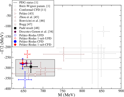
Figure 1: $K_{0}^{*}(700)$ pole positions. Selected from the Review of Particle Physics Tanabashi et al. (2018); Peláez and Rodas (2016); Descotes-Genon and Moussallam (2006); Pelaez (2004b); Zhou and Zheng (2006); Bonvicini et al. (2008); Bugg (2003); Peláez et al. (2017) We also show our results using Roy-Steiner equations, using as input our UFD or CFD parameterizations. Red and blue points use for $F^{-}$ a once-subtracted or an unsubtracted dispersion relation, respectively. This illustrates how unstable pole determinations are when using simple fits to data. Only once Roy-Steiner Eqs. are imposed as a constraint (CFD), both pole determinations fall on top of each other. This final pole position is the main result of this work.

The most sound determination of the $\kappa/K_{0}^{*}(700)$ pole so far is the dispersive analysis by Descotes-Genon et al. Descotes-Genon and Moussallam (2006), also shown in Fig. 1, which uses crossing to implement rigorously the left cut. The pole is obtained using as input a numerical solution in the real axis of Roy-Steiner equations obtained from fixed-$t$ dispersion relations. Unfortunately these fixed-$t$ Roy-Steiner equations do not reach the $\kappa/K_{0}^{*}(700)$-pole region in the complex plane. Remarkably, in Descotes-Genon and Moussallam (2006) it was shown that the $\kappa/K_{0}^{*}(700)$ region is accessible with partial-wave Hyperbolic Dispersion Relations. These were then used to obtain the pole, although starting from the solutions from the fixed-$t$ ones. Note that this is a “solving relations” approach, since no data was used as input in the $\pi K$ elastic region around the nominal $\kappa/K_{0}^{*}(700)$ mass, but only data from other channels and other energies as boundary conditions to the integral equations. In this sense, Descotes-Genon and Moussallam (2006) provides a model-independent prediction. Despite this rigorous result, the $\kappa/K_{0}^{*}(700)$ still “Needs Confirmation”, and we were encouraged by RPP members to carry out an alternative dispersive analysis using data, as previously done by our group for the $\sigma/f_{0}(500)$ García-Martín et al. (2011b). The present work, which follows a “constraining data” approach instead of a “solving relations” approach, provides such an analysis.

It is worth noticing that the $\kappa/K_{0}^{*}(700)$ pole is consistent with $\pi K$ scattering lattice calculations Dudek et al. (2014); Brett et al. (2018). For unphysical pion masses of $\sim 400\,$MeV, it appears as a “virtual” pole below threshold in the second Riemann sheet, consistently with expectations from unitarized NLO ChPT extrapolated to higher masses Nebreda and Pelaez. (2010). However, using pion masses between 200 and 400 MeV the pole extraction using simple models is again unstable Wilson et al. (2019). This makes the approach followed in the present work even more relevant, since in the future lattice will provide data at physical masses and energies around the $\kappa/K_{0}^{*}(700)$ region that will require a “constraining data” technique for a model-independent description and its complex plane continuation.

Let us then describe our approach. In Peláez and Rodas (2016) we first provided Unconstrained Fits to $\pi K$ Data (UFD) up to 2 GeV, for partial waves $f^{I}_{\ell}(s)$ of definite isospin $I$ and angular momentum $\ell$, paying particular attention to the inclusion of systematic uncertainties. As usual, the total isospin amplitude $F^{I}(s,t,u)$, where $s,t,u$ are the Mandelstam variables, is the sum of the partial-wave series. It was then shown that they did not satisfy well Forward Dispersion Relations (FDRs, $t=0$). However, we used these FDRs as constraints to obtain a set of Constrained Fits to Data (CFD), satisfying FDRs up to 1.6 GeV while still describing fairly data fairly well. Note that our “conformal CFD” parameterization of the low-energy isospin 1/2 scalar-wave already contains a $\kappa/K_{0}^{*}(700)$ pole, shown in Fig. 1. This is still a model-dependent extraction from a particular parameterization only valid up to $\sim 1$ GeV.

Later on Peláez et al. (2017), we used sequences of Padé approximants built from the CFD fit to extract a new pole. This “Padé result” in Fig. 1 does not assume any relation between pole position and residue, thus reducing dramatically the model dependence. The value came out consistent within uncertainties with the dispersive result in Descotes-Genon and Moussallam (2006) and triggered the recent change of name in the 2018 RPP edition from $K_{0}^{*}(800)$ to $K_{0}^{*}(700)$. However, it is not fully model independent, since the Padé series is truncated and cuts are mimicked by poles.

Thus, we present here the $\kappa/K_{0}^{*}(700)$ pole obtained from a full analysis of data constrained to satisfy not only FDRs as in Peláez and Rodas (2016), but also both the $S$ and $P$ partial-wave (Roy-Steiner) dispersion relations. The latter are obtained either from fixed-$t$ or Hyperbolic Dispersion Relations (HDR), along $(s-a)(u-a)=b$ hyperbolae, where $s,u$ are the usual Mandelstam variables. In Descotes-Genon and Moussallam (2006) it was shown that the convergence region of the latter in the $a=0$ case reaches the $\kappa/K_{0}^{*}(700)$ pole.

The price of using partial-wave dispersion relations is that they require input from the crossed channel $\pi\pi\rightarrow K\bar{K}$, whose partial waves $g^{I}_{\ell}$ have the same two problems of being frequently described with models and the existence of two incompatible data sets (see Pelaez and Rodas (2018) for details). In addition, there is an “unphysical” region between the $\pi\pi$ and $K\bar{K}$ thresholds, where data do not exist, but is needed for the calculations. Fortunately, Watson’s Theorem implies that the phase there is the well-known $\pi\pi$ phase shift, which allows for a full reconstruction of the amplitude using the Mushkelishvili-Omnés method. Thus, in Pelaez and Rodas (2018) we rederived the HDR partial-wave projections both for $\pi\pi\rightarrow K\bar{K}$ and $\pi K\rightarrow\pi K$, but choosing the center of the hyperbolas in the $s,t$ plane to maximize their applicability region. Once again we found that simple fits to data do not satisfy well the dispersive representation, but we were able to provide constrained parameterizations of the two existing sets describing $S$-wave data up to almost 2 GeV, consistently with HDR up to 1.47 GeV within uncertainties. These are called CFD_B and CFD_C and are part of our input for the $\pi K$ HDR, although we have checked that using one or the other barely changes the $\kappa/K_{0}^{*}(700)$ pole. Note that, contrary to previous calculations, we also provide uncertainties for $\pi\pi\rightarrow K\bar{K}$. Those for the $g^{1}_{1}$ wave are very relevant for the $\kappa/K_{0}^{*}(700)$ pole, particularly in the unphysical region, where there is no data to compare with and the dispersive output leads to two different solutions when using one or no subtractions. Thus, we have also imposed in our CFD that the once and non-subtracted outputs should be consistent within uncertainties, which had not been done in previous calculations.

For our purposes, the most relevant partial wave is $f^{1/2}_{0}$ whose UFD is shown in Fig. 2. As explained in Peláez and Rodas (2016) this wave is obtained by fitting data measured in the $f^{1/2}_{0}+f^{3/2}_{0}/2$ and $I=3/2$ combinations Cho et al. (1970); Bakker et al. (1970); Linglin et al. (1973); Jongejans et al. (1973); Estabrooks et al. (1978); Aston et al. (1988). It is also relevant that, as shown in Fig.2, the $I=1/2$ vector wave UFD describes well the scattering data, in contrast to the solution Descotes-Genon and Moussallam (2006). The rest of the unconstrained partial-waves and high-energy input parameterizations are described in Peláez and Rodas (2016) for $\pi K$ and Pelaez and Rodas (2018) $\pi\pi\rightarrow K\bar{K}$. Minor updates will be detailed in a forthcoming publication Peláez and Rodas .

Figure 2: CFD versus UFD phase shifts $\delta^{I}_{\ell}$ of $f^{1/2}_{0}(s)$ (top) and $f^{1/2}_{1}(s)$ (bottom).

However, as seen in the upper panel of Fig.3 when the UFD is used as input, the dispersive representation is not satisfied within uncertainties. Actually, the fixed-$t$ HDR output does not lie too far from the UFD input, but the outputs using an unsubtracted or once-subtracted HDR for $F^{-}\equiv(F^{1/2}-F^{3/2})/3$ come on opposite sides and far from the input UFD parameterization.

It is now very instructive to see how unstable is the pole parameter extraction from one fit that looks rather reasonable, as the UFD does. Thus, in Fig.1 we show the $\kappa/K_{0}^{*}(700)$ pole position calculated either using the HDR without subtractions for $F^{-}$ (hollow blue) or with one subtraction (hollow red). Note that we use the same UFD input in the physical regions but the two poles come out incompatible. This is mostly due to the pseudo-physical region of the $g^{1}_{1}$ partial wave. The extraction would be even more unreliable if a simple model parameterization was used for the continuation to the complex plane instead of using a dispersion relation.

Thus, in order to obtain a rigorous and stable pole determination, we have imposed that the dispersive representation should be satisfied within uncertainties when fitting data. To this end, we have followed our usual procedure García-Martín et al. (2011a); Peláez and Rodas (2016); Pelaez and Rodas (2018), defining a $\chi^{2}$-like distance $\hat{d}^{2}$ between the input and the output of each dispersion relation at many different energy values, which is then minimized together with the data $\chi^{2}$ when doing the fits.

We minimize simultaneously 16 dispersion relations. Two of them are the FDRs we already used in Peláez and Rodas (2016). Four HDR are considered for the $\pi\pi\rightarrow K\bar{K}$ partial waves: Namely, once subtracted for $g^{0}_{0}$, $g^{0}_{2},g^{1}_{1}$ and another unsubtracted for $g^{1}_{1}$, as we did in Pelaez and Rodas (2018). Note that here we also consider the once-subtracted case for $g^{1}_{1}$. In addition we now impose ten more dispersion relations within uncertainties for the $S$ and $P$ $\pi K$ partial-waves. Four of them come from fixed-$t$ and hyperbolic once-subtracted dispersion relations for $F^{+}\equiv(F^{1/2}+2F^{3/2})/3$, whereas the other six are two fixed-$t$ and another four HDR for $F^{-}$, either non-subtracted or once-subtracted. The HDRs applicability region in the real axis was maximized in Pelaez and Rodas (2018) choosing $a=-13.9m_{\pi}^{2}$. We will however use here $a=-10m_{\pi}^{2}$ as it still has a rather large applicability region in the real axis and ensures that the $\kappa/K_{0}^{*}(700)$ pole and its uncertainty fall inside the HDR domain. For the $\pi K$ $S^{1/2}$-wave, most of the dispersive uncertainty comes from the $\pi K$ $S$-waves themselves when using the subtracted $F^{-}$, whereas a large contribution comes from $g^{1}_{1}$ for the unsubtracted.

The details of our technique have been explained in Peláez and Rodas (2016); Pelaez and Rodas (2018). The resulting Constrained Fits to Data (CFD) differ slightly from the unconstrained ones, but still describe the data. This is illustrated in Fig. 2, were we see that the difference between UFD and CFD is rather small for the $P$-wave, both providing remarkable descriptions of the scattering data. In contrast, in Fig. 2 we see that the CFD $S$-wave is lower than the UFD around and below the $\kappa/K_{0}^{*}(700)$ nominal mass, but still describes well the experimental information. Also, Table 1 shows how the $S$-wave scattering lengths change from the UFD to the CFD. Note that our CFD values are consistent with previous dispersive predictions Buettiker et al. (2004), confirming some tension between data and dispersion theory versus recent lattice results Miao et al. (2004); Beane et al. (2006); Flynn and Nieves (2007); Fu (2012); Sasaki et al. (2014); Helmes et al. (2018). Including those lattice values together with data leads to constrained fits satisfying dispersion relations substantially worse.

Table 1: $S$-wave scattering lengths ($m_{\pi}$ units).

	UFD	CFD	Ref. Buettiker et al. (2004)
$a^{1/2}_{0}$	0.241$\pm$0.012	0.224$\pm$0.011	0.224$\pm$0.022
$a^{3/2}_{0}$	-0.067$\pm$0.012	-0.048$\pm$0.006	-0.0448$\pm$0.0077

Other waves suffer small changes from UFD to CDF, but are less relevant for the $\kappa/K_{0}^{*}(700)$ (see Peláez and Rodas ). All in all, we illustrate in the lower panel of Fig.3 that when the CFD is now used as input of the dispersion relations the curves of the input and the three outputs agree within uncertainties.

Figure 3: Different dispersive outputs for the $f^{1/2}_{0}(s)$ partial wave, versus the input from the data parameterization. Upper panel: Unconstrained Fits to Data (UFD). Note the huge discrepancies between the curves. Lower panel: Constrained Fits to Data (CFD). Now all curves agree within uncertainties. We only show the Roy Steiner results for $f^{1/2}_{0}(s)$ because these are the ones relevant for the $\kappa/K_{0}^{*}(700)$, but the CFD consistency is very good for the other dispersion relations and partial waves. Namely, the average $\chi^{2}/$dof per dispersion relation is 0.7, whereas the average $\chi^{2}/$dof is 1.4 per fitted partial wave.

With all dispersion relations well satisfied we can now use our CFD as input in the HDR and look for the $\kappa/K_{0}^{*}(700)$ pole. Results are shown in Fig.1, this time as solid blue and red symbols depending on whether they are obtained with the unsubtracted or the once-subtracted $F^{-}$. Contrary to the UFD, the agreement between both determinations when using the CFD set is now remarkably good. Precise values of the pole position and residue for our subtracted and unsubtracted results are listed in Table 2, together with the dispersive result of Descotes-Genon and Moussallam (2006) and our Padé sequence determination Peláez and Rodas (2017).

Now, let us recall that the unsubtracted result depends strongly on the $\pi\pi\to K\bar{K}$ pseudo-physical region, particularly on $g^{1}_{1}$, whose unsubtracted dispersion relation error band is almost twice as big as the subtracted one. Moreover, under the change of $a$, the subtracted result, both in the real axis and for the pole, barely changes, whereas the unsubtracted one only changes slightly (a few MeV for the pole). Therefore although both are compatible, we consider the once-subtracted case more robust and thus our final result.

Let us remark that our dispersive pole obtained from data also agrees with the solution in Descotes-Genon and Moussallam (2006), although our width uncertainties are larger. In part, this is because we have estimated uncertainties for all our input.

For completeness, we have also calculated the parameters of the vector $K^{*}(892)$ pole, since we also describe the data there. We find: $\sqrt{s_{p}}=(890\pm 2)-i(25.6\pm 1.2)\,$MeV and its dimensionless residue $|g|=5.69\pm 0.12$.

In summary, we have shown that simple, unconstrained fits to the existing $\pi K$ and $\pi\pi\rightarrow K\bar{K}$ data fail to satisfy hyperbolic and fixed-$t$ dispersion relations and yield rather unreliable $\kappa/K_{0}^{*}(700)$ pole determinations. However, we have obtained fits to data constrained to satisfy those two hyperbolic dispersion relations, together with other Forward and fixed-$t$ dispersion relations. These constrained fits provide a rigorous, precise and robust determination of the $\kappa/K_{0}^{*}(700)$ pole parameters. We think these results should provide the needed confirmation that, according to the Review of Particle Physics and the hadronic community, was needed to establish firmly the existence and properties of the $\kappa/K_{0}^{*}(700)$.

Table 2: Poles and residues of the $\kappa/K_{0}^{*}(700)$. The last two lines are our dispersive outputs. The last line is our final result.

	$\sqrt{s_{pole}}$   (MeV)	$|g|$   (GeV)
$K^{*}_{0}(700)$ Descotes-Genon and Moussallam (2006)	$(658\pm 13)-i(279\pm 12)$	—
$K^{*}_{0}(700)$ Peláez et al. (2017)	$(670\pm 18)-i(295\pm 28)$	4.4$\pm$0.4
$K^{*}_{0}(700)$ 0-sub	$(648\pm 6)-i(283\pm 26)$	3.80$\pm$0.17
$\bf{K^{*}_{0}(700)}$ 1-sub	$\bf{(648\pm 7)-i(280\pm 16)}$	$\bf{3.81\pm 0.09}$

Acknowledgments

This project has received funding from the Spanish MINECO grant FPA2016-75654-C2-2-P and the European Union’s Horizon 2020 research and innovation programme under grant agreement No 824093 (STRONG2020). AR would like to acknowledge the financial support of the U.S. Department of Energy contract DE-SC0018416 and of the Universidad Complutense de Madrid.

References

- Tanabashi et al. (2018) M. Tanabashi et al. (Particle Data Group), Phys. Rev. D98, 030001 (2018).
- Johnson and Teller (1955) M. H. Johnson and E. Teller, Phys. Rev. 98, 783 (1955).
- Schwinger (1957) J. S. Schwinger, Annals Phys. 2, 407 (1957).
- Jaffe (1977) R. L. Jaffe, Phys.Rev. D15, 267 (1977).
- Jaffe (2007) R. L. Jaffe, Proceedings, 4th International Workshop on QCD - Theory and Experiment (QCD@Work 2007), AIP Conf.Proc. 964, 1 (2007), [Prog.Theor.Phys.Suppl.168,127(2007)], arXiv:hep-ph/0701038 [hep-ph] .
- Pelaez (2004a) J. R. Pelaez, Phys. Rev. Lett. 92, 102001 (2004a), arXiv:hep-ph/0309292 [hep-ph] .
- Pelaez and Yndurain (2005) J. R. Pelaez and F. J. Yndurain, Phys. Rev. D71, 074016 (2005), arXiv:hep-ph/0411334 [hep-ph] .
- Pelaez (2016) J. R. Pelaez, Phys. Rept. 658, 1 (2016), arXiv:1510.00653 [hep-ph] .
- Londergan et al. (2014) J. T. Londergan, J. Nebreda, J. R. Peláez, and A. Szczepaniak, Phys.Lett. B729, 9 (2014), arXiv:1311.7552 [hep-ph] .
- Peláez and Rodas (2017) J. R. Peláez and A. Rodas, Eur.Phys.J. C77, 431 (2017), arXiv:1703.07661 [hep-ph] .
- Peláez and Rodas (2016) J. R. Peláez and A. Rodas, Phys. Rev. D93, 074025 (2016), arXiv:1602.08404 [hep-ph] .
- Roy (1971) S. M. Roy, Phys.Lett. 36B, 353 (1971).
- Ananthanarayan et al. (2001a) B. Ananthanarayan, G. Colangelo, J. Gasser, and H. Leutwyler, Phys.Rept. 353, 207 (2001a), arXiv:hep-ph/0005297 [hep-ph] .
- Colangelo et al. (2001) G. Colangelo, J. Gasser, and H. Leutwyler, Nucl. Phys. B603, 125 (2001), arXiv:hep-ph/0103088 [hep-ph] .
- Descotes-Genon et al. (2002) S. Descotes-Genon, N. H. Fuchs, L. Girlanda, and J. Stern, Eur. Phys. J. C24, 469 (2002), arXiv:hep-ph/0112088 [hep-ph] .
- Kaminski et al. (2003) R. Kaminski, L. Lesniak, and B. Loiseau, Phys. Lett. B551, 241 (2003), arXiv:hep-ph/0210334 [hep-ph] .
- García-Martín et al. (2011a) R. García-Martín, R. Kamiński, J. R. Peláez, J. Ruiz de Elvira, and F. J. Ynduráin, Phys.Rev. D83, 074004 (2011a), arXiv:1102.2183 [hep-ph] .
- Kaminski (2011) R. Kaminski, Phys. Rev. D83, 076008 (2011), arXiv:1103.0882 [hep-ph] .
- Moussallam (2011) B. Moussallam, Eur. Phys. J. C71, 1814 (2011), arXiv:1110.6074 [hep-ph] .
- Caprini et al. (2012) I. Caprini, G. Colangelo, and H. Leutwyler, Eur. Phys. J. C72, 1860 (2012), arXiv:1111.7160 [hep-ph] .
- Albaladejo et al. (2018) M. Albaladejo, N. Sherrill, C. Fernández-Ramírez, A. Jackura, V. Mathieu, M. Mikhasenko, J. Nys, A. Pilloni, and A. P. Szczepaniak, Eur.Phys.J. C78, 574 (2018), arXiv:1803.06027 [hep-ph] .
- Steiner (1971) F. Steiner, Fortsch. Phys. 19, 115 (1971).
- Ditsche et al. (2012) C. Ditsche, M. Hoferichter, B. Kubis, and U. G. Meissner, JHEP 06, 043 (2012), arXiv:1203.4758 [hep-ph] .
- Hoferichter et al. (2016) M. Hoferichter, J. Ruiz de Elvira, B. Kubis, and U.-G. Meißner, Phys. Rept. 625, 1 (2016), arXiv:1510.06039 [hep-ph] .
- Colangelo et al. (2019) G. Colangelo, M. Hoferichter, and P. Stoffer, JHEP 02, 006 (2019), arXiv:1810.00007 [hep-ph] .
- Hoferichter et al. (2011) M. Hoferichter, D. R. Phillips, and C. Schat, Eur. Phys. J. C71, 1743 (2011), arXiv:1106.4147 [hep-ph] .
- Moussallam (2013) B. Moussallam, Eur. Phys. J. C73, 2539 (2013), arXiv:1305.3143 [hep-ph] .
- Danilkin and Vanderhaeghen (2019) I. Danilkin and M. Vanderhaeghen, Phys. Lett. B789, 366 (2019), arXiv:1810.03669 [hep-ph] .
- Hoferichter and Stoffer (2019) M. Hoferichter and P. Stoffer, JHEP 07, 073 (2019), arXiv:1905.13198 [hep-ph] .
- Johannesson and Nilsson (1978) N. Johannesson and G. Nilsson, Nuovo Cim. A43, 376 (1978).
- Ananthanarayan and Buettiker (2001) B. Ananthanarayan and P. Buettiker, Eur. Phys. J. C19, 517 (2001), arXiv:hep-ph/0012023 [hep-ph] .
- Ananthanarayan et al. (2001b) B. Ananthanarayan, P. Buettiker, and B. Moussallam, Eur. Phys. J. C22, 133 (2001b), arXiv:hep-ph/0106230 [hep-ph] .
- Buettiker et al. (2004) P. Buettiker, S. Descotes-Genon, and B. Moussallam, Eur. Phys. J. C33, 409 (2004), arXiv:hep-ph/0310283 [hep-ph] .