GG Tau A: gas properties and dynamics from the cavity to the outer disk

Abstract

Context. GG Tau A is the prototype of a young triple T Tauri star that is surrounded by a massive and extended Keplerian outer disk. The central cavity is not devoid of gas and dust and at least GG Tau Aa exhibits its own disk of gas and dust emitting at millimeter wavelengths. Its observed properties make this source an ideal laboratory for investigating planet formation in young multiple solar-type stars.

Aims. We used new ALMA ${}^{13}{\rm CO}$  and C¹⁸O(3–2) observations obtained at high angular resolution ($\sim 0.2^{\prime\prime}$) together with previous CO(3–2) and (6–5) ALMA data and continuum maps at 1.3 and 0.8 mm in order to determine the gas properties (temperature, density, and kinematics) in the cavity and to a lesser extent in the outer disk.

Methods. By deprojecting, we studied the radial and azimuthal gas distribution and its kinematics. We also applied a new method to improve the deconvolution of the CO data and in particular better quantify the emission from gas inside the cavity. We perform local and nonlocal thermodynamic equilibrium studies in order to determine the excitation conditions and relevant physical parameters inside the ring and in the central cavity.

Results. Residual emission after removing a smooth-disk model indicates unresolved structures at our angular resolution, probably in the form of irregular rings or spirals. The outer disk is cold, with a temperature $<20$ K beyond 250 au that drops quickly ($\propto r^{-1}$). The kinematics of the gas inside the cavity reveals infall motions at about 10% of the Keplerian speed. We derive the amount of gas in the cavity, and find that the brightest clumps, which contain about 10% of this mass, have kinetic temperatures $40-80$ K, CO column densities of a few $10^{17}$ cm^-2, and H₂ densities around $10^{7}$ cm^-3.

Conclusions. Although the gas in the cavity is only a small fraction of the disk mass, the mass accretion rate throughout the cavity is comparable to or higher than the stellar accretion rate. It is accordingly sufficient to sustain the circumstellar disks on a long timescale.

1 Introduction

In more than two decades of studying exoplanets, nearly 4,000 exoplanets have been found. More than 10% of these planets are detected in binary or higher hierarchical systems (Roell et al. 2012). The general picture of planet formation is well agreed: planets are formed within a few million years after the collapse phase in a protoplanetary disk surrounding the protostar. However, the detailed formation conditions and mechanisms are still debated.

Welsh et al. (2012) reported observations with the Kepler space telescope and revealed that planets can form and survive in binary systems, on circumbinary or circumstellar orbits. The formation conditions in these systems differ from those around single stars. Theoretical studies of disk evolution predict that the stars in a T Tauri binary of about 1 Myr should be surrounded by two inner disks, that are located inside the Roche lobes, and by an outer ring or disk that is located outside the outer Lindblad resonances (Artymowicz et al. 1991). For a binary system of low or moderate eccentricity, the stable zone is typically located beyond the 3:1 or 4:1 resonance (Artymowicz & Lubow 1994). The residual gas and dust inside the nonstable zone inflows from the circumbinary to the circumstellar disks through streamers (Artymowicz et al. 1991), feeding inner disks that otherwise would not survive. The outer radii of these inner disks, as well as the inner radius of the circumbinary (outer) disk, are defined by tidal truncation. At (sub)millimeter wavelengths, circumbinary disks have been observed in many systems, and in some of these, such as L 1551 NE, UY Aur and GG Tau A (Takakuwa et al. 2014; Tang et al. 2014; Dutrey et al. 2014), the circumstellar disk(s) is also detected. Studying the gas and dust properties in these environments is a necessary step for understanding the formation of planets in the binary/multiple systems.

The subject of this paper is a detailed study of gas and dust properties of the GG Tau A system. GG Tau A, located in the Taurus-Auriga star-forming region consists of a single star GG Tau Aa and the close binary GG Tau Ab1/Ab2 with separations of 35 au and 4.5 au on the plane of the sky, respectively (Dutrey et al. 2016; Di Folco et al. 2014). We here ignore the binary nature of Ab, and only consider the GG Tau Aa/Ab binary, unless explicitly noted otherwise. Although the GAIA results suggest a value of 150 pc (Gaia Collaboration et al. 2016; Brown et al. 2018), we use a distance of 140 pc for comparison with previous works.

The triple star is surrounded by a Keplerian disk that is tidally truncated inside at $\sim$180 au. The disk is comprised of a dense gas and dust ring that extends from about 180 au up to 260 au and an outer disk that extends out to $\sim$800 au (Dutrey et al. 1994). The disk is inclined at about $35^{\circ}$, with a rotation axis at PA $7^{\circ}$. The Northern side is closest to us (Guilloteau et al. 1999). The disk is one of the most massive in the Taurus region, $\sim$0.15 M_⊙. This is $\sim$10% of the total mass of the stars. A 10% mass ratio should lead to a small deviation (about 5%) from the Keplerian law (Huré et al. 2011) outside the ring.

The outer disk is relatively cold and has dust and gas (derived from ¹³CO analysis) temperatures of 14 K and 20 K at 200 au, respectively (Dutrey et al. 2014; Guilloteau et al. 1999). More information about the triple system can be found in Dutrey et al. (2016) and the references therein.

We here present a study of GG Tau A using sub-millimeter observations carried out with ALMA. The main goal is to derive the properties of the gas cavity (density, temperature, and kinematics). For this purpose, we use a simple model for the gas and dust outer disk that allows us to better retrieve the amount of gas inside the cavity and simultaneously provides interesting information about the outer gas disk. The paper is organized as follows. Section 2 describes the observations and data reduction. The observation results are presented in Section 3, and the radiative transfer modeling of the outer disk is presented in Section 4. The properties of the cavity (excitation conditions, mass, and dynamics) are derived in Section 5. The gas and dust properties in the circumbinary disk and inside the tidal cavity are discussed in Section 6. Section 7 summarizes the main results.

2 Observations and data reduction

Table 1 lists the observational parameters of our data sets: the spectral sampling, angular resolution and brightness sensitivity for all observed molecular lines.

Table 1: List of observations

Spectral line	Frequency	Energy level	Channel spacing	Beamsize	Noise
	(GHz)	(K)	(km/s)		(K)	ALMA project
12CO(6–5)	691.473	33.2	0.106	$0.35^{\prime\prime}\times 0.31^{\prime\prime}$, PA=$104^{\circ}$	1.8	2011.0.00059.S
12CO(3–2)	345.795	16.6	0.106	$0.34^{\prime\prime}\times 0.28^{\prime\prime}$, PA=$91^{\circ}$	0.7	2012.1.00129.S
13CO(3–2)	330.588	15.9	0.110	$0.22^{\prime\prime}\times 0.16^{\prime\prime}$, PA=$15^{\circ}$	0.7	2012.1.00129.S, 2015.1.00224.S
C18O(3–2)	329.330	15.8	0.110	$0.19^{\prime\prime}\times 0.14^{\prime\prime}$, PA=$19^{\circ}$	1.9	2015.1.00224.S
Continuum	330.15	–	–	$0.19^{\prime\prime}\times 0.14^{\prime\prime}$, PA=$10^{\circ}$	0.03	2015.1.00224.S

GG Tau A was observed with ALMA Band 9 during Cycle 0 (2011.0.00059.S) and Band 7 during Cycle 1 (2012.1.00129.S) and Cycle 3 (2015.1.00224.S). Anne Dutrey is the PI of the three projects.

Cycle 0

Observations were made on 2012 August 13. The spectral windows covered the ¹²CO(6–5) line (see Dutrey et al. 2014, for details of the data reduction). These data were processed here with a restoring beam of $0.35^{\prime\prime}\times 0.31^{\prime\prime}$ at PA=$104^{\circ}$.

Cycle 1

Observations were taken on 2013 November 18 and 19. The spectral windows covered the lines of ¹²CO(3–2) and ¹³CO(3–2) at high spectral resolution ($0.11\,\,{\rm km\,s}^{-1}$). Details of data reduction are given in Tang et al. (2016). The ¹²CO(3–2) images were obtained here with a restoring beam of $0.34^{\prime\prime}\times 0.28^{\prime\prime}$ at PA=$-89^{\circ}$, and the ¹³CO(3–2) data were merged with new data acquired in Cycle 3.

Cycle 3

Observations were carried on 2016 September 25 and 30 with 37 and 38 useful antennas in configuration C40-6. The projected baselines range from 16 m to 3049 m, and the total time on source is 1.4 hours. The spectral setup covered the lines of ¹³CO(3–2) and C¹⁸O(3–2) at 330.588 and 329.330 GHz in two windows, each covering 58.89 MHz bandwidth with a high spectral resolution of 141 kHz ($\sim$0.11 $\,{\rm km\,s}^{-1}$). The continuum was observed in two separate windows, one centered at 330.15 GHz with 1875 MHz bandwidth and the other centered at 342.00 GHz with 117 MHz bandwidth.

Data were calibrated with the CASA software (version 4.7.0). We used the quasar J0510+1800 for phase and bandpass calibration. The absolute amplitude calibration was made using J0522-3627 (flux $\sim$3.84 Jy at 343.5 GHz at the time of observations). The calibrated data were regrided in velocity to the local standard of rest (LSR) frame using the task cvel, and were exported through UVFITS format to the GILDAS package for further data processing.

GG Tau has significant proper motions: Ducourant et al. (2005) cited $[17,-19]$ mas per year, while Frink et al. (1997) reported $[11,-28]$ mas per year. These measurements are affected by the multiplicity of the star, however. To realign our observations, we assumed that the continuum ring is centered on the center of mass of the system which we took as the center of coordinates for our images. We fit the continuum emission with the sum of a circular Gaussian (for the circumstellar disk around Aa) and an elliptical ring (for the dust ring) in the $uv$ plane (Guilloteau et al. 1999; Piétu et al. 2011). The apparent motion of the ring gives a proper motion of $[9,-23]$ mas per year, which we applied to all our data set. With these proper motions, the origin of the coordinates is at RA=4h 32m 30.3s and DEC=$17^{\circ}\,31^{\prime}\,40^{\prime\prime}$ at epoch 2000.

The imaging and deconvolution was made with natural weighting, and the images were cleaned down to the rms noise level with the $hogbom$ algorithm Channel maps of the observed lines are presented in Appendix A, Figs.12–13. In these data, the maximum recoverable scale is about 7^′′ (1000 au at the source distance). The images were not corrected for primary beam attenuation: the beam size of 17^′′ yields attenuation of 12% at 500 au and 4% at 300 au.

3 Results

3.1 Continuum emission

Figure 1 shows the continuum emission at 330 GHz derived from the Cycle 3 data. It reveals emission from the Aa disk and the ring structure detected in previous observations (see Dutrey et al. 2016, and references therein), but the ring is now clearly resolved. The ring is not azimuthally symmetric (after taking the limb-brightening effect along the major axis into account), but displays a $\sim$15-20% stronger emission at $\rm{PA}\approx$$240^{\circ}-260^{\circ}$. The outer edge is clearly shallower than the steep inner edge, confirming that some dust remains beyond the $\sim$260 au outer edge of the ring, as initially mentioned by Dutrey et al. (1994). As in previous studies (e.g., Guilloteau et al. 1999; Piétu et al. 2011), compact, unresolved emission is detected in the direction of the single star Aa, but no emission originates from the Ab close binary system.

A detailed study of the continuum emission is beyond the scope of this paper and is deferred to subsequent work.

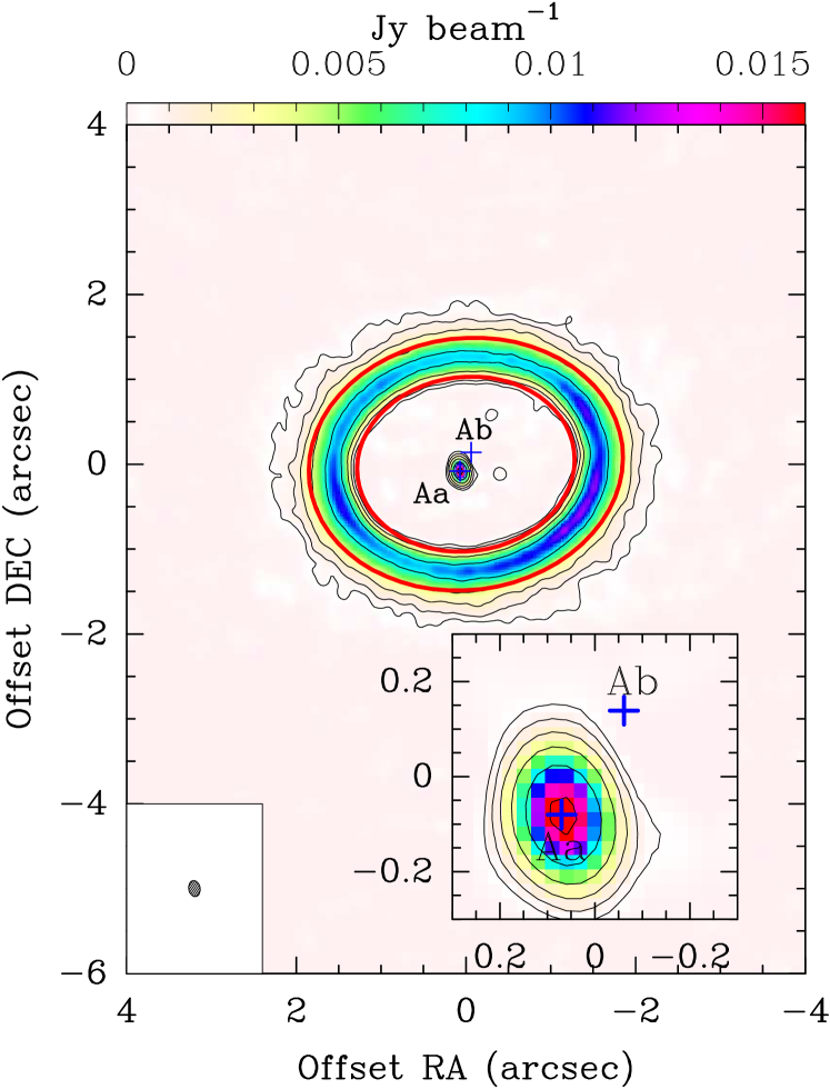
Figure 1: Continuum image at 330 GHz. The beam size of $0.19^{\prime\prime}\times 0.14^{\prime\prime},\rm{PA}=190^{\circ}$ is indicated in the lower left corner. The contour levels are 0.5, 1, 2, 4, 8 and 16 mJy beam^-1. The noise level is 0.06 mJy beam^-1. The red ellipses indicate the inner and outer edges of the dense dust ring at 180 au and 260 au, respectively (e.g., Guilloteau et al. 1999). The positions of the Aa star and Ab close binary are indicate by the crosses. The inset shows an enlarged view of the Aa and Ab surroundings.

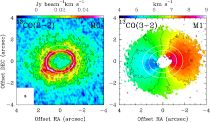
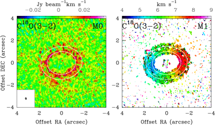
Figure 2: Upper: ¹³CO(3–2) integrated intensity map (left, contour spacing 0.01 Jy/beam km s^-1 (3 $\sigma$) with zero level omitted) and velocity map (right). Lower: C¹⁸O(3–2) integrated intensity map (left, contour spacing 0.01 Jy/beam km s^-1, 2 $\sigma$) and velocity map (right).The beams are indicated in lower left corner in each intensity map. The contour level spacing in the velocity maps is $0.5\,{\rm km\,s}^{-1}$. The continuum has been subtracted. The white ellipses indicate the inner and outer edges of the dust ring.

3.2 Images of line emission

Figure 2 shows the integrated intensity and the velocity maps of ¹³CO(3–2) (left) and C¹⁸O(3–2) (right). In these figures, the continuum has been subtracted. The velocity fields suggest Keplerian rotation inside the disk.

The ¹³CO(3–2) emission extends out to 550 au, and the C¹⁸O(3–2) is mostly visible in the dense ring.

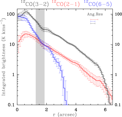
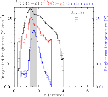
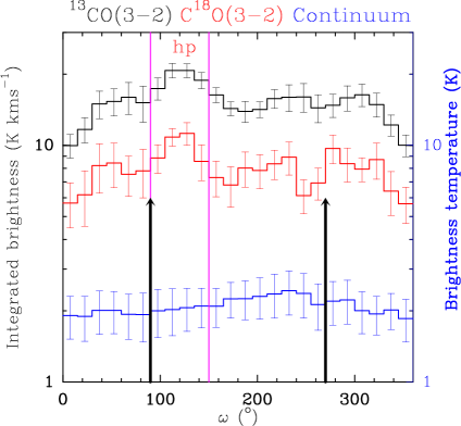
Figure 3: Upper panels: Radial dependence of the integrated brightness temperature (for lines) and brightness temperature (for continuum emission) in the disk plane. The horizontal sticks indicate the angular resolutions. Lower panels: Azimuthal dependence of the same quantities averaged over the ring of $1.2^{\prime\prime}<r<2.0^{\prime\prime}$. The left panels show the plot of the emission from the J=6–5, 3–2 and 2–1 lines of ¹²CO. For a description of the corresponding data, see Tang et al. (2016) for the J=3–2 line and Dutrey et al. (2014) for the others. The right panels show the less abundant CO isotopologs (J=3–2) emissions. The gray region delineates the dust ring in the upper panels. In the lower panels, black arrows show the location of the limb-brightening peaks and the magenta lines show the hot-spot location.

3.2.1 Intensity variations

Figure 3 (upper panels) shows the radial profiles of the integrated brightness of the lines and of the peak brightness of the continuum emission, averaged over the entire azimuthal direction, after deprojection to the disk plane. The deprojection was made assuming a position angle of the minor disk axis of 7^∘ and an inclination of 35^∘ (Dutrey et al. 2014; Phuong et al. 2018b). See also Phuong et al. (2018b) for a detailed description of the deprojection.

The ¹²C¹⁶O emission covers a broad region around the central binary, $r\apprle 6^{\prime\prime}$ (800 au), peaking at the center. Some of the differences between the three transitions of CO may result from calibration effects and different $uv$ coverage. In particular, short spacings are missing in the CO(6–5) transition data because of its high frequency, making it less sensitive to extended structures.

Figure 3 (lower panels) displays the azimuthal dependence (in the disk plane) of the peak brightness and velocity-integrated brightness in the ring ($1.2^{\prime\prime}\leq r\leq 2^{\prime\prime}$) for CO, ¹³CO, C¹⁸O and the 0.85 mm continuum emissions. The azimuth $\omega$ in the disk midplane is measured counterclockwise from the minor axis, with 0 in the north direction. The significant enhancement in the southeastern quadrant for ¹²C¹⁶O corresponds to the hot spot discovered by Dutrey et al. (2014), which may reveal a possible planet in formation (labelled “hp” for hypothetical planet in the figure). It is far fainter in the other CO isotopologs.

3.2.2 CO gas kinematics in the outer disk

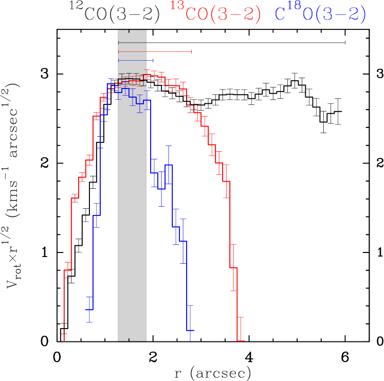
Figure 4: Dependence on $r$ of $V_{rot}\times\,r^{1/2}$ (weighted by the brightness and averaged in bins of $0.15^{\prime\prime}$) of ¹²CO(3–2) (black), ¹³CO(3–2) (red) and C¹⁸O(3–2) (blue) emissions. The horizontal bars indicate the radius range over which the mean value is computed for each transition. The gray shaded area indicates the boundaries of the dense dust ring.

For a thin disk, the line-of-sight velocity is given by $V_{z}=\sin i(V_{rot}\sin\omega+V_{fall}\cos\omega)$ where $i$ is the disk inclination, $V_{rot}$ the rotation velocity and $V_{fall}$ the infall velocity, and $\omega$ is the azimuth in the disk plane. We can neglect the infall motions, because the studies of Phuong et al. (2018b) at angular resolution of $\sim 0.35^{\prime\prime}$ have placed an upper limit of 9% on it with respect to the rotation. We used the intensity-weighted images of the line-of-sight velocity $V_{z}$ shown in Fig.2 and for each pixel calculate $V_{z}(\sin i\sin\omega)^{-1}$. We then azimuthally averaged these values for all pixels at the same radius (using a $0.15^{\prime\prime}$ radial binning) such that $|\sin\omega|$ to $>0.7$ (i.e., avoiding pixels around the minor axis) to derive $V_{rot}$.

Figure 4 shows the dependence of $\langle V_{rot}\,(r/1^{\prime\prime})^{1/2}\rangle$ on $r$, which would be constant for the three CO isotopologs if the rotation were Keplerian. The overall agreement between the three isotopes is good, showing that the outer ring and disk are in Keplerian rotation beyond about 180 au. A constant fit to these histograms gives $V_{rot}\approx 2.94\,{\rm km\,s}^{-1}$, with a standard deviation ($\sigma$) of $0.14\,{\rm km\,s}^{-1}$ of the residuals from the mean for CO, $2.98\,{\rm km\,s}^{-1}$ ($\sigma=0.04\,{\rm km\,s}^{-1}$) for ¹³CO and $2.81\,{\rm km\,s}^{-1}$ ($\sigma=0.07\,{\rm km\,s}^{-1}$) for C¹⁸O, at $\approx 1.0^{\prime\prime}$ (the integration ranges are illustrated in Fig.4).

The formal errors on these mean values are two to three times smaller, depending on the number of independent points, which is not a simple value given our averaging method. However, the CO data show deviations from the mean that are not random, because they occur on a radial scale of $\approx 0.8^{\prime\prime}$, more than twice the resolution. We therefore conservatively used the standard deviation as the error on the mean. Using the three independent measurements from CO, ¹³CO, and C¹⁸O, we derive a mean weighted value of $2.94\pm 0.03\,{\rm km\,s}^{-1}$ for the Keplerian rotation speed at $1^{\prime\prime}$, i.e. $3.48\pm 0.04\,{\rm km\,s}^{-1}$ at 100 au, in agreement with previous, less precise determinations (e.g. Dutrey et al. (2014) found $3.4\pm 0.1\,{\rm km\,s}^{-1}$). When the uncertainty on the inclination, $\pm 2^{\circ}$, is taken into account, this corresponds to a total stellar mass of $1.36\pm 0.07{\,\rm M}_{\odot}$.

The apparent lower-than-Keplerian velocities for radii larger than $2.1^{\prime\prime}$ (for C¹⁸O) or $3^{\prime\prime}$ (for ¹³CO) are due to the low level of emission in these transitions. Those at radii smaller than about $0.8^{\prime\prime}$ are discussed in Sec.6.3.

4 Disk modeling

4.1 Objectives

Our main objective is to derive the properties of the gas in the cavity. However, the overall source size, in CO and ${}^{13}{\rm CO}$, is comparable to or larger than the largest angular scale that can be recovered. This means that a simple method in which we would just use the globally deconvolved image to identify the emission from the cavity might be seriously affected by the missing extended flux. Accordingly, we used a more elaborate approach in which we fit a smooth-disk model to the emission beyond about 160 au. The extended emission from this model is better recovered through its analytic prescription. This outer disk model was later subtracted from the visibility data, so that the residuals have no structures at scales larger than about 3.5^′′, that is, the cavity size. These residuals can then be properly imaged and deconvolved without suffering from missing large-scale flux.

4.2 Disk model

We used the DiskFit tool (Piétu et al. 2007) to derive the bulk properties of the ring and outer disk. The disk model was that of a flared disk with piece-wise power laws for the temperatures and surface densities, and sharp inner and outer radii beyond which no molecule (or dust) exists. The temperature was vertically isothermal, and the vertical density profile was a Gaussian, $n(r,z)=n_{0}(r)\exp(-(z/H(r))^{2})$, with a scale height following a simple power law $H(r)=h_{0}(r/R_{0})$. For spectral lines, we assumed that the velocity field was Keplerian, $v(r)=V_{0}(r/R_{0})^{-0.5}$, and used a constant local line width $dV$. The lines are assumed to be at local thermal equilibrium (LTE): the derived temperatures thus indicate excitation temperatures. The emission from the disk was computed using a ray-tracing method. The difference between the predicted model visibilities and the observed ones is minimized using a Levenberg–Marquardt method, and the error bars were derived from the covariance matrix.

A more detailed description of the DiskFit tool and our adopted fitting method is given in Appendix B. The fit parameters are summarized in Table 8.

4.3 Continuum fit

The CO emission being at least partially optically thick, we cannot simply separate the contribution of CO and continuum (Weaver et al. 2018). To determine the continuum properties, we fit the continuum using the broadband, line-free spectral window data. We followed the procedure described in Dutrey et al. (2014), who derived dust properties using 1.3 mm and 0.45 mm continuum. We first subtracted a Gaussian source model of the emission from the circumstellar disk of Aa. The emission from the ring was then fit by a simple power-law distribution for the surface density and temperature, with sharp inner and outer edges (see also Appendix B), assuming a spatially constant dust absorption coefficient that scales with frequency $\nu$ as $\nu^{\beta}$.

The goal of this continuum modeling is that residual emission after model fitting becomes lower than the noise level in the spectral line data, so that the continuum does not introduce any significant bias in the combined fit for spectral lines described in the next section. It is enough to adjust only the surface density for this. We thus fixed geometrical parameters (center, position angle, and inclination, see Table 2) and the inner and outer radii, the absorption coefficient, and the temperature profile, using the results of Dutrey et al. (2014). The results of the continuum fit are given in Table 3. The residuals, such as those due to the $\simeq 20$ % azimuthal variations visible in Fig.1, or the shallow outer edge of the brightness distribution, are well below 1 K in brightness.

Table 2: System geometric and kinematic parameters

Parameter	Value
$(x_{0},y_{0})$	(0,0)	Center of dust ring	fixed
$PA(^{\circ})$	$7$	PA of disk rotation axis	fixed
$i(^{\circ})$	$-35$	Inclination	fixed
$V_{\mathrm{LSR}}$ ($\,{\rm km\,s}^{-1}$)	6.40	Systemic velocity	fixed
$V_{0}$ (km s${}^{-1})$	$3.37$	Keplerian velocity at 100 au	fixed
$dV$ (km s${}^{-1})$	$0.3$	Local line width	fixed

Table 3: Dust ring parameters

Parameter	Value/Law
Inner radius (au)	193	fixed
Outer radius (au)	285	fixed
Abs. coefficient $\kappa_{\nu}$ (cm${}^{2}/g$)	$0.02\times(\nu/230\mathrm{GHz})^{+1}$	fixed
Temperature (K)	$14\times(r/200\mathrm{\,au})^{-1}$	fixed
Surface density (cm-2)	5.6 $10^{24}\times(r/200\mathrm{\,au})^{-1.4}$	Fitted

4.4 CO isotopologs

We analyzed the CO isotopolog data without removing the continuum. The parameters labeled “fixed” in Tables 2 - 3 were used as fixed input parameters for our modeling.

While the outer disk is well represented by a Keplerian disk, the emission from the cavity does not follow such a simple model. It contributes to a significant fraction of the total emission from CO, however. Because the fit was made by minimizing in the visibility (Fourier) plane, we cannot separate the cavity from the contributions of outer disk in this process.

To avoid biasing our results for the ring and disk parameters, we therefore adopted a specific strategy. We first subtracted the Clean components located inside the cavity (up to a radius of 160 au) from the original $uv$ tables (this also removes the continuum from Aa). The modified $uv$ tables were then analyzed using an innerly truncated Keplerian disk model, as described in detail in Appendix B.

Because the radial profiles of the emission from CO and ¹³CO are not well represented by a power law (see Fig.3, and Fig.3 of Tang et al. 2016), our disk model assumes piece-wise, continuous power laws (linear in log-log space) for the surface density and temperature. We used knots at 160, 200, 260, 300 and 400 au. The knots were chosen to reflect both the slope changes in the radial profile of the line emissions and the sharp edges of the dust ring based on our previous studies (Dutrey et al. 1994; Guilloteau et al. 1999), and to allow a good estimate for the properties of the bulk of the gas in the ring and outer disk using a minimum of knots.

The following strategy was adopted to fit in parallel the ${{}^{12}{\rm CO}}$ and ${{}^{13}{\rm CO}}$ data. In a first step, we determined the temperature by fitting the ${{}^{12}{\rm CO}}$ line. The surface density of CO is not a critical value here: because CO is largely optically thick, we just need to use a high enough CO surface density to ensure this. We then used this temperature profile to fit the ${{}^{13}{\rm CO}}$ data and determine the ${{}^{13}{\rm CO}}$ surface density, because this line is partially optically thin. The derived surface density was then multiplied by the isotopic ratio ${{}^{12}{\rm CO}}/{{}^{13}{\rm CO}}$ (70, Milam et al. 2005) to specify the CO surface density to iterate on the temperature determination using the ${{}^{12}{\rm CO}}$ data. The process converges quickly (in two iterations).

Our method makes the underlying assumption that the ${{}^{12}{\rm CO}}$ and ${{}^{13}{\rm CO}}$ layers are at the same temperature. This hypothesis is consistent with the results from Tang et al. (2016), who found that the vertical temperature gradient around $200-400$  au needs to be small to reproduce the observed ${{}^{12}{\rm CO}}/{{}^{13}{\rm CO}}$ line ratio.

A fixed inner radius of 169 au provided a good compromise to represent all molecular distributions. This radius is here only to obtain a good model for the ring and outer disk: it should not be overinterpreted as the physical edge of the cavity. We also independently determined the outer radii for each CO isotopolog, and verified the best-fit value for the inclination and systemic velocity. The small difference between our adopted Keplerian rotation law and the law suggested by the analysis in Sec.3.2.2 has negligible effect on the fitted parameters. For the C¹⁸O, we used only four knots to derive the surface density profile.

With this process, we find a reasonable model of the ring and outer disk in all CO isotopologs. Figure 5 shows the residuals from the original $uv$ data after removal of the best-fit outer disk models and of Aa continuum source. As expected, most of the left-over emission is coming from the cavity, but some azimuthal asymmetries are still visible in the dense ring and beyond (e.g. the hot spot and low level extended emission). The best fit results and formal errors are summarized in Table 4, Figure 6, and Figure 7. Significant deviations from the best fit model do exist (e.g., azimuthal variations), therefore the results must be interpreted with caution. The formal errors underestimate the uncertainties on the physical parameters. We therefore also quote a confidence interval for the temperatures in Table 4, based on the dispersion of values found during our minimization studies: surface densities are typically uncertain by $20-30$%, but the steep decrease in temperature between 200 and 300 au, and then to 400 au and beyond is a robust result. The surface density profile around $180-200$ au is poorly constrained, because emission inside 160 au was removed, and the angular resolution at this level is insufficient. However, the variations in the fitted surface densities between 169 au (the inner truncation radius) and 180 au suggest a very dense inner edge.

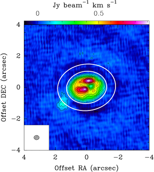
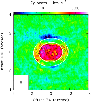
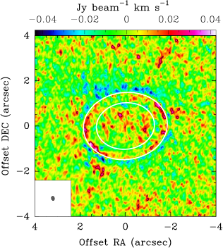
Figure 5: Integrated intensity of (residual) emissions after subtracting the best ring+disk models. Left: ${{}^{12}{\rm CO}}$(3–2). The restoring beam of $0.34^{\prime\prime}\times 0.28^{\prime\prime},\rm{PA}=-89^{\circ}$ is indicated in the lower left corner. Middle: ${{}^{13}{\rm CO}}$(3–2). The restoring beam is $0.22^{\prime\prime}\times 0.16^{\prime\prime},\rm{PA}=16^{\circ}$. Right: C¹⁸O(3–2). The restoring beam is $0.19^{\prime\prime}\times 0.14^{\prime\prime},\rm{PA}=-167^{\circ}$. The contour level is 0.07 Jy beam^-1 km s^-1 (5$\sigma$) for ${{}^{12}{\rm CO}}$(3–2) map and $\sim$0.02 Jy beam^-1 km s^-1 (3$\sigma$) for ${{}^{13}{\rm CO}}$(3–2) and ${{\rm C}^{18}{\rm O}}$(3–2) maps, the zero level is omitted. The ellipses show the inner and outer edges of the dust ring at 180 and 260 au.

In spite of its limitations, our approach leads to some conclusions. Beyond a radius of about 200 au, the CO gas is cold and temperatures drop from about 27 K at 180 au to 11 K at 400 au (see Fig.6) (or about 13 K after correction for primary beam attenuation).

We note that the scale height of $24$ au at 200 au that was found to represent well the CO isotopolog emissions (see Appendix B) corresponds to a kinetic temperature of 15 K under the hyothesis of hydrostatic equilibrium. This agrees reasonably well with the dust temperature derived by Dutrey et al. (2014).

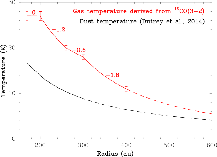
Figure 6: Radial dependence of CO gas (red) and dust (black) temperature. The gas temperature is derived from the ${{}^{12}{\rm CO}}$(3–2) analysis. Beyond 400 au, CO temperature is extrapolated from the fitted law in the range of $300-400$ au. The power-law exponents are indicated in each range. The uncertainty on the exponent is about 0.15 for the best constrained values (-1.2 and -1.8), and 0.3 for the others. The primary beam attenuation introduces a bias of $8\%$ at 400 au. The dust temperature is taken from Dutrey et al. (2014). Beyond a radius of 285 au, the dust temperature corresponds to an extrapolation.

The outer radius of the disk is $370$ au in ${{\rm C}^{18}{\rm O}}$, about 550 au in ${{}^{13}{\rm CO}}$ and greater than 600 au in ${{}^{12}{\rm CO}}$. The last two radii are less well constrained than that of ${{\rm C}^{18}{\rm O}}$ because the temperature drops steeply with radius.

Table 4: Temperature derived from ¹²CO(3–2) and surface density from ¹³CO(3–2) and ${{\rm C}^{18}{\rm O}}$(3–2)

(1)	(2)	(3)	(4)	(5)	(6)	(7) )
r	Tk			13CO	C18O	Ratio
(au)	(K)	(K)	(K)	$10^{15}$ cm-2
160	$27.2$	$0.17$	[26,28]	$39\pm 2$	$6.7\pm 0.6$	$5.8\pm 0.8$
200	$27.4$	$0.11$	[25,28]	$18\pm 1$	$5.5\pm 0.4$	$3.3\pm 0.4$
260	$19.7$	$0.07$	[19,21]	$9.7\pm 0.3$	$2.1\pm 0.1$	$4.6\pm 0.4$
300	$18.0$	$0.03$	[17,19]	$6.8\pm 0.1$	$0.39\pm 0.02$	$17\pm 1$
400	$10.7$	$0.02$	[10,12]	$2.8\pm 0.03$	–	–

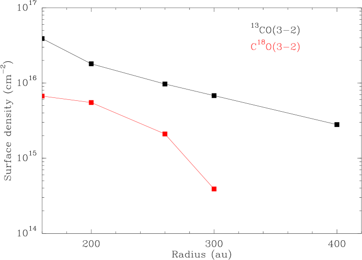
Figure 7: Comparison of the surface densities from the LTE analysis.

5 Analysis of the gas inside the cavity

With a good first-order model for the spectral line emission in the ring and outer disk (i.e. beyond 169 au), we can now determine a better representation of the emission coming from the gas in the cavity. For this purpose, we subtracted our best ring+disk model (presented in Sec. 4) from the original visibilities. CLEANed images of this residual emission, which mostly comes from the cavity, were produced for the three CO isotopologs (¹²CO, ¹³CO and C¹⁸O J=3–2). Figure 5 presents the residual maps obtained. In this section, we study the properties of the gas inside the cavity using these residual maps.

5.1 Dynamics inside the cavity

To study the gas dynamics inside the cavity, we plot in Fig.8 the azimuthal dependence of $\langle V_{z}/\sin(i)\rangle$ in five rings of width $0.25^{\prime\prime}$ each of ¹²CO(3–2), ¹³CO(3–2), and C¹⁸O(3–2) emissions in the region $0<r<1.25^{\prime\prime}$. Azimuth and radius are defined in the disk plane, i.e. deprojected from the disk inclination. In each ring, we fit the azimuthal dependency of $\langle V_{z}/\sin(i)\rangle$ of the ${{}^{13}{\rm CO}}$ with a sine function $V_{z}/\sin(i)=V_{z0}\sin\omega$. This sine function is presented as the smooth red curve and the amplitude $V_{z0}$ is provided at the top of each panel. The good fit for the ${{}^{13}{\rm CO}}$(3–2) indicates that the gas inside the cavity is dominated by rotation. The amplitude is smaller than that of the Keplerian velocity $v(r)=\sqrt{GM_{tot}/r}$, however, where $M_{tot}$ is the total mass of the stars. However, this is most likely a result of the finite resolution of the observations combined with the very inhomogeneous brightness distribution. The dynamics of the three lines agree for $1^{\prime\prime}<r<1.25^{\prime\prime}$, but differ in the region with $r<1^{\prime\prime}$. In particular, the ${{}^{12}{\rm CO}}$(3–2) departs from the ${{}^{13}{\rm CO}}$(3–2) in the region $0.25^{\prime\prime}<r<1^{\prime\prime}$ (boxes (b,c,d) in Fig.8) because of the bright localized emission regions seen in CO.

However, a better fit to the observed velocities is obtained by taking into account the contribution of a radial (from the disk center) velocity $V_{z}/\sin(i)=V_{fall}\cos\omega+V_{rot}\sin\omega$. The results are presented in Table 5: $V_{fall}>0$ corresponds to infall motions. As an example, the improvement in fit quality is shown for the range $0.5^{\prime\prime}<r<0.75^{\prime\prime}$ in panel (f) of Fig.8. Table 5 thus indicates that the gas in the cavity moves inwards to the center at velocities about $0.3\,\,{\rm km\,s}^{-1}$, which is about $10-15\%$ of the Keplerian velocity. Because infall and rotation motions have different radial and azimuthal dependencies, the finite beam size has a different effect on the infall velocity than on the apparent rotation velocity, especially in the presence of brightness inhomogeneities.

Table 5: Infall and rotation velocities of the gas inside the cavity.

Ring	$V_{Kep}$	$V_{rot}$	$V_{fall}$	$\frac{V_{fall}}{V_{rot}}$	$\frac{V_{fall}}{V_{Kep}}$
	($\,{\rm km\,s}^{-1}$)	($\,{\rm km\,s}^{-1}$)	($\,{\rm km\,s}^{-1}$)
(a)	-	0.34	0.04	12%	-
(b)	-	0.79	0.21	27%	-
(c)	3.63	0.98	0.30	31%	8%
(d)	3.07	1.08	0.38	28%	12%
(e)	2.71	1.27	0.48	38%	18%

A direct illustration of the infall motions is given in Fig.9, which shows position-velocity (PV) diagrams of the ${{}^{13}{\rm CO}}$(3–2) emission in the cavity along the major and minor axis of the disk. The PV diagram along the major axis shows the Keplerian rotation down to the inner edge of the ${{}^{13}{\rm CO}}$(3–2) emission, at $\sim 1.1^{\prime\prime}$ ($160$ au). The PV diagram along the minor axis shows an asymmetry between the north and the south consistent with the derived infall motion of $\sim 0.3-0.4\,{\rm km\,s}^{-1}$ at the same (deprojected) radius (the PV diagrams are presented in the sky plane).

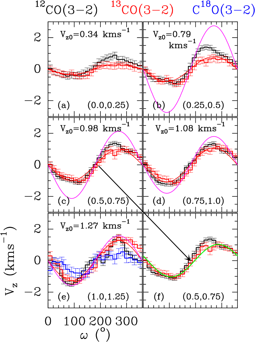
Figure 8: Dependence of $\langle V_{z}\rangle$ ($\,{\rm km\,s}^{-1}$) on the azimuth $\omega$ (^∘) in the cavity. ¹²CO (3–2) is in black, ¹³CO (3–2) in red and C¹⁸O (3–2) in blue. The red curve is a fit of a sine function to the ¹³CO (3–2) data (see text). We use a blank space when no good data are available (no emission) in the ring. The magenta curves show the expected Keplerian velocity around a single star of 1.36 M_⊙. The green curve in panel (f) shows the best-fit velocity curve when infall motions are allowed, superimposed on the ¹³CO velocity.

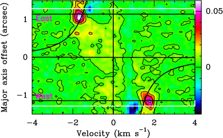
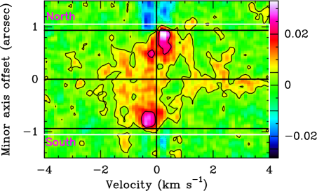
Figure 9: Position-velocity diagrams of the ${{}^{13}{\rm CO}}$(3–2) emission in the cavity along the major (upper panel) and minor axis (lower panel). The black curves show the expected Keplerian velocity around a single star of $1.36\,\mathrm{M}_{\odot}$. Contour levels are spaced by 10 mJy/beam; the zero contour is omitted. The white lines indicate the position of the inner edge of the dust ring (180 au) and the black lines show the position of the inner radius of the gas disk (169 au). The data were rotated by $7^{\circ}$ to align with the disk axis, so that cardinal directions are approximate.

5.2 Gas properties

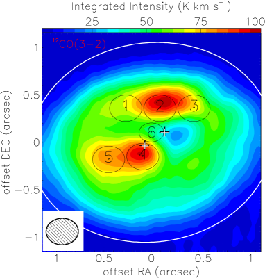
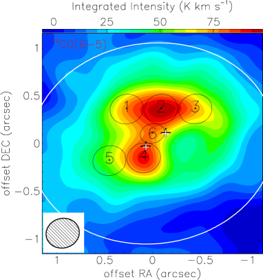
Figure 10: Integrated intensity map of ${{}^{12}{\rm CO}}$(3–2) (upper) (this work and Tang et al. 2016) and ${{}^{12}{\rm CO}}$(6–5) (lower) (from Dutrey et al. 2014) and positions and sizes of the blobs. The crosses mark the positions of Aa and Ab, and the ellipse is the inner edge of the dust ring (180 au).

Using the (residual) ${{}^{12}{\rm CO}}$(3–2) data and the ¹²CO(6–5) data from Dutrey et al. (2014), for which the emission outside of the cavity is negligible, smoothed to a similar angular resolution ($0.35^{\prime\prime}\times 0.30^{\prime\prime}$), we identify 2 dominant features. We decomposed these strong emission regions into five independent beams (“blobs”) that we analyzed separately. To this we added a sixth blob that connected blobs 2 and 4, a region that is particularly bright in CO(6–5) (see Figure 10). Integrated line flux and line width were derived for each blob by fitting a Gaussian to the line profile. Velocities and line width derived from the CO (3–2) were used to determine the ¹³CO and C¹⁸O line intensities.

Table 6: Properties of the brighter blobs

Blob	Position	Radius	$dv$	H2 density	N	Tkin	Mass (nLTE)	Mass (${{}^{12}{\rm CO}}$ Flux)	Mass (${{}^{13}{\rm CO}}$ Flux)
	(${}^{\prime\prime},^{\prime\prime}$)	(′′)	($\,{\rm km\,s}^{-1}$)	(cm-3)	(cm-2)	(K)	($\,\mathrm{M}_{\odot}$)	($\,\mathrm{M}_{\odot}$)	($\,\mathrm{M}_{\odot}$)
(1)	( 2)	(3)	(4)	(5)	(6)	(7)	(8)	(9)	(10)
1	(0.27, 0.36)	0.45	2.5	$>5.0\,10^{4}$	$(2.1^{+0.6}_{-0.7})\,10^{17}$	$40\pm 5$	$(2.1^{+0.6}_{-0.7})\,10^{-6}$	$(3.1\pm 0.1)\,10^{-7}$	$(1.9\pm 0.1)\,10^{-6}$
2	($-$0.09, 0.36)	0.37	2.7	$>1.0\,10^{4}$	$(1.4^{+0.7}_{-0.5})\,10^{17}$	$50\pm 5$	$(1.3^{+0.7}_{-0.5})\,10^{-6}$	$(4.5\pm 0.1)\,10^{-7}$	$(2.3\pm 0.1)\,10^{-6}$
3	($-$0.45, 0.36)	0.58	2.1	$>5.0\,10^{4}$	$(2.6^{+1.0}_{-1.00})\,10^{17}$	$40\pm 5$	$(2.5^{+1.0}_{-1.0})\,10^{-6}$	$(3.2\pm 0.2)\,10^{-7}$	$(1.1\pm 0.1)\,10^{-6}$
4	(0.09, $-$0.15)	0.17	6.2	$>1.0\,10^{5}$	$(6.3^{+2.1}_{-1.4})\,10^{16}$	$80\pm 10$	$(6.3^{+2.1}_{-1.4})\,10^{-7}$	$(6.9\pm 0.1)\,10^{-7}$	$(2.5\pm 0.2)\,10^{-6}$
5	(0.45, $-$0.18)	0.48	2.5	$>1.0\,10^{4}$	$(2.2^{+1.0}_{-0.8})\,10^{17}$	$40\pm 5$	$(2.2^{+1.0}_{-0.8})\,10^{-6}$	$(3.9\pm 0.1)\,10^{-7}$	$(1.7\pm 0.1)\,10^{-6}$
6	(0, 0.1)	0.12	6.1	$>1.0\,10^{4}$	$(4.0^{+1.4}_{-1.4})\,10^{16}$	$80\pm 10$	$(4.0^{+1.4}_{-1.4})\,10^{-7}$	$(3.4\pm 0.1)\,10^{-7}$	$(2.8\pm 0.1)\,10^{-6}$

To determine the physical conditions, we used a non-LTE escape probability radiative transfer code implemented in DiskFit. It uses the escape probability formulation of Elitzur (1992), $\beta=[1-\exp(-\tau)]/\tau$, a single collision partner, H₂, and Gaussian line profiles. Non-LTE best-fit solutions were found by sampling the $\chi^{2}$ surface, which is defined as the quadratic sum of the difference between the measured brightness temperatures and the computed values of the CO (6–5), CO (3–2), ¹³CO (3–2), and C¹⁸O (3–2) transitions, for ranges of H₂ density of $10^{2}-10^{10}$ cm^-3, ${{}^{12}{\rm CO}}$ column density of $10^{13}-10^{19}$ cm^-2, and kinetic temperature of $3-100$ K using 50 steps of each parameter. We assumed the standard isotopic ratios ¹²C/¹³C$=70$ (Milam et al. 2005) and ¹⁶O/¹⁸O$=550$ (Wilson 1999) for the relative abundances of the isotopologs. ${{}^{12}{\rm CO}}$ constrains the temperature, and ${{}^{13}{\rm CO}}$ the column densities. Owing to its faintness, the C¹⁸O(3–2) data bring little information. Because the critical densities of the observed transitions are low, we only obtain a lower limit to the density. The blob parameters are presented in Table 6.

We typically find high CO column densities of about a few $\sim 10^{17}$ cm^-2 and temperatures in the range 40–80 K, with a lower limit on the density of about 10⁵ cm^-3. For blob 6, the faintest region analyzed with this method, the problem is marginally degenerate, with two separate solutions: i) a high column density ($\sim 10^{17}$ cm^-2) and low temperature ($\sim 20$ K), and (ii) a low column density ($\sim 10^{15}$ cm^-2) and high temperature ($>80$ K). This region lies between Aa and Ab, therefore the second solution (which is also that of lowest $\chi^{2}$) is more probable.

5.3 Gas masses

The lower limit on the density obtained from the non-LTE analysis was insufficient to provide any useful constraint on the blob masses, we therefore used another method. We estimated the blob mass from the derived molecular column density and blob size, assuming a molecular abundance relative to H₂, as described below.

In the same way, we also derived the total amount of gas in the cavity from the integrated flux of the optically thin lines of the ¹³CO(3–2) and C¹⁸O(3–2). For this purpose, we integrated the emission out to a radius of 160 au.

In the optically thin approximation, the integrated flux and the column density of the upper level of a given transition are related by

$$W=\frac{g_{u}}{\gamma_{u}}N_{u}\\ \\$$ (1)

where $W=\int{T_{b}\,dv}$ is the integrated brightness inside the cavity ($R<160$ au), $g_{u}=2J+1$ is the statistics weight and $N_{u}$ is the column density of the upper level, $\gamma_{u}=\frac{hc^{3}A_{ul}}{8\pi\,k_{B}\nu^{2}}$ (the Einstein coefficient $A_{ul}$ is taken from Lamda database). Guided by the results of the non-LTE analysis, we assumed that the gas temperature $T$ is 40 K everywhere inside the cavity and calculated the total column density $N_{\textnormal{total}}$ of a given molecule as

$$N_{\textnormal{total}}=\frac{N_{u}}{Z}\exp\left(\frac{-E_{u}}{k_{B}\,T}\right)$$ (2)

where, $Z$ is the partition function and $E_{u}$ is the energy of the upper state. The ¹²CO(3–2) emission, which is partially optically thick, yields a lower limit.

The CO abundance was taken from the abundances measured in TMC-1 by Ohishi et al. (1992), and we assumed a standard isotopic ratio for the isotopologs (${{}^{13}{\rm CO}}$ and ${{\rm C}^{18}{\rm O}}$). The results are listed in Cols 9-10 of Table 6 for the blobs, and Table 7 summarizes the results for the cavity.

Table 7: Mass of gas inside the cavity

Location	Integrated Flux	H2 mass	Abundance
	(Jy $\,{\rm km\,s}^{-1}$)	($\,\mathrm{M}_{\odot}$)	(w.r.t H2)
Cavity (${{}^{12}{\rm CO}}$)	$11.4\pm 0.8$	$6.1\pm 0.4\times 10^{-6}$	$8.0\times 10^{-5}$
Cavity (${{}^{13}{\rm CO}}$)	$3.8\pm 0.1$	$1.6\pm 0.1\times 10^{-4}$	$\dagger$
Cavity (${{\rm C}^{18}{\rm O}}$)	$0.5\pm 0.2$	$1.6\pm 0.8\times 10^{-4}$	$\ddagger$

The H₂ mass derived from ${{}^{13}{\rm CO}}$(3–2) and C¹⁸O(3–2) is similar which confirms that these lines are optically thin while the ${{}^{12}{\rm CO}}$ emission is optically thick.

6 Discussion

Figure 11 is a schematic layout summarizing the properties of the GG Tau A system. Numbers quoted in this schematic view are discussed in the following section.

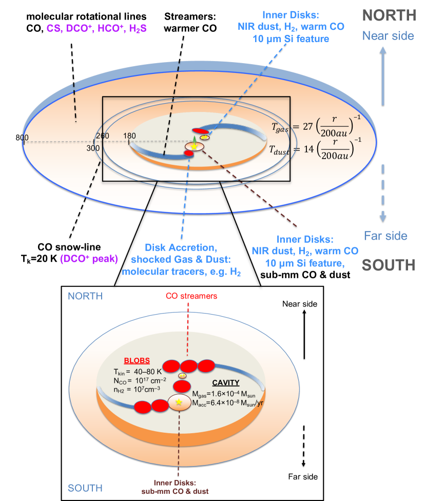
Figure 11: Schematic view of the GG Tau system. Colored text indicates results obtained from other publications. In particular, magenta shows results from Phuong et al. (2018a); see Dutrey et al. (2016) for a review of other references. Black text shows results from this work.

6.1 Temperature distribution in the outer disk

Our analysis confirms that most of the outer disk of GG Tau A is very cold (see Fig.6). The gas temperature derived here agrees with the value found by Guilloteau et al. (1999) from ${{}^{13}{\rm CO}}$ alone, 20 K at 300 au. The agreement between values derived independently from ${{}^{12}{\rm CO}}$ and ${{}^{13}{\rm CO}}$ supports our assumption of a limited vertical temperature gradient in the CO layer, as already mentioned by Tang et al. (2016). A power-law fit to this temperature profile gives a radial dependency of $r^{-1}-r^{-1.3}$, confirming the previous exponent value of $-1$ derived by Guilloteau et al. (1999). Dutrey et al. (2014) also found a similar exponent for the dust temperature from the analysis of dust images between 3 and 0.45 mm using a simple power law. Because this study is based on multi-wavelength continuum resolved observations from 3 up to 0.45 mm, the derived dust temperature is characteristic of the large grains that have likely settled down around the midplane. It is then reasonable to consider that this temperature traces the midplane dust temperature. This steep radial slope of the temperatures is most likely due to the stellar light that is blocked by the inner dense ring, and the rest of the disk then remains in its shadow.

6.2 Gas distribution and smoothness of the outer ring

Global properties

Our canonical (smooth) model (Sec.4.4) shows that the ratio of the ${{}^{13}{\rm CO}}$ and ${{\rm C}^{18}{\rm O}}$ column densities beyond $r>300$ au is about 17 (see Table 4) above the standard isotopic ratio of 7, suggesting selective photodissociation (e.g., van Dishoeck & Black 1988), but also confirming that in the outer disk the emissions are optically thin.

In contrast, inside the densest part of the ring ($200-260$ au), the measured ratio is about $3-5$. Chemical effects such as selective photodissociation and fractionation which occurs through isotope exchange between CO and C⁺ (Watson et al. 1976) and enhances ¹³CO at temperatures of about 20-30 K, would both tend to enhance this ratio above the double isotopic (¹⁶O/¹⁸O)/(¹²C/¹³C) ratio. Thus the simplest explanation for a low value is partially optically thick ${{}^{13}{\rm CO}}$(3–2) emission. However, our model should account for the opacity if the disk were as smooth as assumed. We therefore conclude that the GG Tau disk and ring deviate significantly from the smooth, nonstratified, azimuthally symmetric structure we adopted.

Smoothness versus unresolved structures

The radial profile (see the upper panels in Fig.3) of the observed molecular lines, ${{}^{12}{\rm CO}}$(3–2), ${{}^{13}{\rm CO}}$(3–2), and C¹⁸O(3–2) does not appear smooth. After subtracting the best (smooth) outer disk model, Figure 5 reveals some additional emission that is located in rings at specific azimuths. This is particularly clear for the optically thinner transitions of the C¹⁸O(3–2), suggesting radial density variations in the molecular layer (at about one scale height). In contrast to the gas, the dust emission is hardly visible in the outer disk (radius $>260$ au), but mostly concentrated in the ring (radius $200-260$ au).

The azimuthal dependence of the integrated brightness of the ¹²C¹⁶O emission (lower left panel in Fig.3) shows strong excesses at specific azimuths. The excess seen in the south-east quadrant is consistent with the hot-spot location quoted by Dutrey et al. (2014). This hot spot remains visible, but less clearly so in ${{}^{13}{\rm CO}}$ and ${{\rm C}^{18}{\rm O}}$. This indicates that it is mostly a temperature enhancement, and not an overdensity region.

In the residual maps (Fig.5), other azimuthal variations are also visible. Our smooth model removes any azimuthally symmetric emission so that apparent effects resulting from velocity coherence length and convolution with elongated beam-shape are properly eliminated. The observed residuals thus reveal intrinsic structures.

All this evidence indicates the existence of radial and azimuthal substructures that remain unresolved (at least radially) at our 30 au linear resolution.

6.3 Properties of the gas inside the cavity

Kinematics

Figure 4 shows that the rotation appears sub-Keplerian at radii smaller than about $0.8^{\prime\prime}$. This could be the signature of the tidal forces generated by the Aa/Ab binary. Unfortunately, this is largely an effect of the intensity drop in the cavity, combined with the finite angular resolution. Because the signal intensity increases with radius in the cavity, the intensity-weighted mean velocity is biased towards the values obtained at the largest radii, i.e. the gas apparently rotates at lower velocities. A proper modeling of the angular resolution effect, accounting for the observed brightness distribution, would be required to remove this artifact and determine whether the gas rotate at the expected Keplerian speed.

On the other hand, we find clear evidence for infall motions in the cavity (see Sec.5.1), at velocities about $10-15\%$ of the Keplerian speed, proving that material is accreting onto the inner disks orbiting the central stars. This is consistent with the infall value found for L 1551 NE, a younger binary system (Takakuwa et al. 2017). However, our sensitivity is insufficient for a detailed comparison with hydrodynamics models.

In summary, we find that the gas starts to exhibit non-Keplerian motions (at least infall motions, and perhaps slower than Keplerian rotation) at $r\approx 160$ au, somewhat smaller than the inner edge of the dust ring (193 au). This difference in radii is expected when dust trapping in the high-pressure bump that occurs in the dense ring is considered (e.g. Cazzoletti et al. 2017). The 160 au radius remains much larger than the radius at which tidal disturbances are expected in a binary system, however. Theoretical studies showed that such disturbances are expected at radius of $2.5-3$ times the major axis of the binary orbit (Artymowicz & Lubow 1996). The binary separation of Aa/Ab, 35 au, means that this theoretical value should be of the order of 100 au. Therefore, we would expect that deviations from Keplerian motions only appear inside about 100 au, unless the orbit is very eccentric. High eccentricity appears unlikely given the measured orbital parameters; see Beust & Dutrey (2005) who also reported that underestimated astrometric error bars might play an important role. Following Beust & Dutrey (2005), Köhler (2011) and Nelson & Marzari (2016) showed that this apparent contradiction could be solved under the assumption that the orbital plane of the stars is very different from the (common) plane of the ring and outer disks. A similar result was found by Aly et al. (2018), who indicated that an inclination difference of 30^∘ could remain stable over the (circumbinary) disk lifetime. However, Brauer et al. (2019) found by studying the projected shadows of the disks in the near IR, that the circumstellar disk around Aa and one of the disks around Ab1 or Ab2 must also be coplanar with the circumbinary ring and disk. This makes the misaligned orbit proposition unlikely, because the alignment of the circumstellar disks is more controlled by the gravitational interactions with the stars than with the (much less massive) outer disk. The cavity size puzzle thus remains.

Gas temperature

Our non-LTE analysis, in agreement with the study from Dutrey et al. (2014), shows that the gas inside the cavity is warm, with temperatures ranging from 30 to 80 K. In the bright blobs, near the stars, we derived a kinetic temperature of about $40-50$ K at about $30-60$ au from the central stars. It is important to mention that these temperatures are well above the CO freeze-out temperature.

Amount of gas

From our non-LTE analysis of the bright blobs, we found a few $10^{17}$ cm^-2 for the CO column density with the exception of blobs 4 and 6, which have a lower column density of $\sim$(3-6)  10¹⁶ cm^-2. We also obtained a lower limit on the H₂ density of about $(1-10)\,10^{4}$ cm^-3 for all blobs. However, a more stringent constraint can be obtained from the blob masses given in Table 6, because the thickness of the blobs is on the order of the scale height $H(r)$, 5 to 10 au at this distance to the stars. This leads to densities about $10^{7}$ cm^-3.

The cumulative mass of the blobs is $\sim 1.2\times 10^{-5}\,\mathrm{M}_{\odot}$. We also estimated the total gas mass inside the cavity from the integrated flux of the optically thin CO isotopologs. We found a mass of $\sim 1.6\times 10^{-4}\,\mathrm{M}_{\odot}$, assuming standard CO abundance (see Table 7). The ${{}^{13}{\rm CO}}$ and ${{\rm C}^{18}{\rm O}}$ values perfectly agree suggesting that both the ${{}^{13}{\rm CO}}$ and ${{\rm C}^{18}{\rm O}}$ emissions are essentially optically thin in the cavity.

Therefore, the total mass of the gas inside the cavity appears to be a factor 10 higher than the cumulative blob mass. This only relies on the assumption of similar molecular abundances in these regions, which is reasonable given their similar temperatures. Thus a significant fraction of the gas in the cavity does not reside in the dense blobs but in diffuse features.

Determining the absolute value of the gas mass inside the cavity is more challenging. On the one hand, our assumed value for the CO abundance, that observed in TMC-1, appears reasonable given the relative high temperature in the cavity. However, lower values might result from C and O still being locked on grains in the form of more complex or less volatile molecules (CO₂ and CH₄, see Reboussin et al. (2015)). A proper quantification of such a process would require a complete chemical study that would follow the physical and chemical evolution of the gas and solid phases throughout the disk.

Nevertheless, an absolute minimum value for the gas mass in the cavity can be obtained when we assume the CO abundance cannot exceed the carbon cosmic abundance expected in cold molecular clouds ($3.4\times 10^{-4}$, Hincelin et al. 2011). In this case, we obtain the minimum mass by correcting the previous value by the factor of $\sim 0.2$. This leads to $\sim 0.3\times 10^{-4}\,\mathrm{M}_{\odot}$ for the total gas mass inside the cavity.

In any case, the mass of gas in the cavity is only a very small fraction of the total disk mass (0.15$\,\mathrm{M}_{\odot}$) that is estimated from the dust emission.

Mass accretion rate

The gas in the cavity is unstable and will accrete onto the GG Tau A disks on a timescale of a few (about four) times the orbital binary period, which is estimated to be about 600 years (see Beust & Dutrey 2005). A similar timescale, about 2500 yr, is given independently by the ratio of cavity radius to the measured infall velocities. This gives an accretion rate of $\sim 6.4\times 10^{-8}\,\mathrm{M}_{\odot}\,\rm{yr}^{-1}$ when we assume the canonical mass value. The accretion rate on GG Tau Aa+Ab, measured in year 2000 using the H_α line, is about $\sim 2\times 10^{-8}\,\mathrm{M}_{\odot}\,\rm{yr}^{-1}$ (Hartigan & Kenyon 2003), a factor 3 lower than our estimate. This small difference (a factor 3) may be essentially due to the limited accuracy of the two methods in use. However, it may also be partly explained by variable accretion inside the cavity and onto the central star(s) associated to non steady-state dynamics. In a binary star, the accretion rate process is modulated by the eccentricity, and is more efficient at the pericenter, with a delay that depends on the eccentricity (Artymowicz & Lubow 1996; Günther & Kley 2002). The two values of the accretion rates may then reflect different aspects of a highly variable process depending how and when these rates are measured. The fair agreement between the two results shows that the GG Tau A disk can be sustained by accretion through the cavity on a long timescale.

7 Summary

We reported new observations of CO isotopologs with ALMA of the close environment of GG Tau A. We studied the ring by performing an LTE analysis, and we performed a non-LTE analysis for the gas clumps observed inside the cavity. We also investigated the gas kinematics in the outer disk and inside the cavity.

The ring and outer disks do not exhibit a smooth distribution, but likely consist of a series of unresolved substructures with some azimuthal variations, particularly in the dense inner ring. The bright hot spot seen in ¹²CO is marginally seen in ${{}^{13}{\rm CO}}$ and in ${{\rm C}^{18}{\rm O}}$, suggesting a temperature effect.

The gas temperature derived from the optically thick CO line has a sharp decrease ($r^{-1}$), as for the dust. The temperature of 20 K (CO snow line) is reached at $\sim$ 300 au.

The total amount of mass inside the cavity derived from ${{}^{13}{\rm CO}}$ is $1.6\times 10^{-4}\,\mathrm{M}_{\odot}$, assuming standard CO abundance.

The gas streamers inside the cavity can essentially be defined by six blobs. A non-LTE analysis reveals that their conditions are similar, with CO column densities of about a few $\sim 10^{17}$ cm^-2, temperatures in the range $40-80$ K, and H₂ density in the dense parts of about 10⁷ cm^-3.

The kinematics of the whole structure (outer ring plus cavity) appears to be in Keplerian rotation around a 1.36 $\,\mathrm{M}_{\odot}$ system for radii beyond $\sim$1.2^′′ or 180 au. The kinematics of the gas streamers and blobs appears more complex than expected for such a binary system. In particular, the gas starts to exhibit non-Keplerian motions for radii smaller than $\sim 160$ au.

The gas inside the cavity shows infall motions of about 10% of the Keplerian velocity, allowing the central stars to accrete material from the dense ring.

The average mass flow rate of the gas through the cavity is $\sim 6\times 10^{-8}\,\mathrm{M}_{\odot}\,\rm{yr}^{-1}$. This value is compatible with the stellar accretion rate measured using the H_α line, and it is sufficient to replenish the circumstellar disks.

Appendix A Channel maps

We present in Figs.12-13 the Cleaned channel maps produced without subtracting the continuum emission.

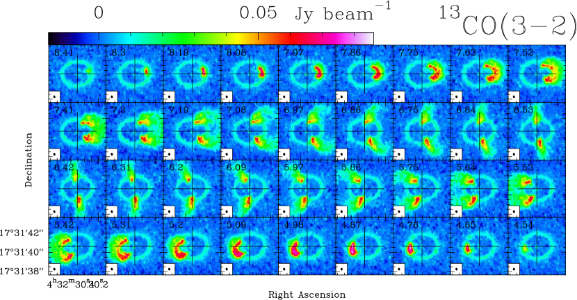
Figure 12: Channel maps of ${{}^{13}{\rm CO}}$(3–2), beam $0.22"\times 0.16"$, PA=$16^{\circ}$. The noise level is 2.4 mJy beam^-1. The color scale is indicated in the upper panels. The cross is centered on the center of the map.

Figure 13: Channel maps of C¹⁸O(3–2), beam $0.19"\times 0.14"$, PA=$19^{\circ}$. The noise level is 4.8 mJy beam^-1. The color scale is indicated in the upper panels. The cross is centered on the center of the map.

Appendix B Disk model fitting

We used the tool DiskFit (Piétu et al. 2007) to derive the physical parameters of rotating circumstellar disks.

Principles:

DiskFit computes the spatial distribution of the emission from spectral lines (and dust) as a function of frequency (related to the line rest frequency and Doppler velocity of the source) for a given azimuthally symmetric disk model.

In its basic form, as described in Piétu et al. (2007), the disk model assumes that the relevant physical quantities that control the line emission vary as power law as a function of radius, and, except for the density, do not depend on height above the disk plane. The exponent is taken as positive when the quantity decreases with radius:

$$a(r)=a_{0}(r/R_{a})^{-e_{a}}.$$ (3)

When dust emission is negligible, the disk for each molecular line is thus described by the following parameters:

• $X_{0},Y_{0}$, the star position, and $V_{\mathrm{disk}}$, the systemic velocity.

• PA, the position angle of the disk axis, and $i$ the inclination.

• $V_{0}$, the rotation velocity at a reference radius $R_{v}$, and $v$ the exponent of the velocity law. With our convention, $v=0.5$ corresponds to Keplerian rotation. Furthermore, the disk is oriented so that the $V_{0}$ is always positive. Accordingly, PA varies between 0 and $360^{\circ}$, while $i$ is constrained between $-90^{\circ}$ and $90^{\circ}$.

• $T_{m}$ and $q_{m}$, the temperature value at a reference radius $R_{T}$ and its exponent.

• $dV$, the local line width, and its exponent $e_{v}$.

• $\Sigma_{m}$, the molecular surface density at a radius $R_{\Sigma}$ and its exponent $p_{m}$

• $R_{\mathrm{out}}$, the outer radius of the emission, and $R_{\mathrm{in}}$, the inner radius.

• $h_{m}$, the scale height of the molecular distribution at a radius $R_{h}$, and its exponent $e_{h}$: it is assumed that the density distribution is Gaussian, with

  $$n(r,z)=\frac{\Sigma(r)}{h(r)\sqrt{\pi}}\exp\left[-\left(z/h(r)\right)^{2}\right]$$ (4)

  (note that with this definition, $e_{h}<0$ in realistic disks),

which gives a grand total of 17 parameters to describe a pure spectral line emission.

All these parameters can be constrained for each observed line under the above assumption of power laws. This comes from two specific properties of protoplanetary disks: i) the rapid decrease in surface density with radius, and ii) the known kinematic pattern. In particular, we can derive both the temperature law ($T_{m},q_{m}$) and the surface density law ($\Sigma_{m},p_{m}$) when there is a region of optically thick emission (in the inner parts) while the outer parts is optically thin.

When dust emission is not negligible, it can also be accounted for in the emission process. Again assuming simple power laws, this adds up six new parameters: two for the dust temperature, two for the dust surface density, and the inner and outer radii of the dust distribution. The absolute value of the dust surface density is degenerate with that of the dust absorption coefficient. Surface density and temperature may also be degenerate if the dust emission is optically thin and in the Rayleigh Jeans regime. Because dust emission is in general weak compared to the observed spectral lines, an inaccurate model of the dust will have limited effects.

Power laws are a good approximation for the velocity, temperature (see, e.g., Chiang & Goldreich 1997), and thus to the scale height prescription. For molecular surface density, the approximation may be less good because of chemical effects.

We refer to Piétu et al. (2007) for a more thorough discussion of the interpretation of the model parameters. We recall, however, that the temperature derived in this way for a molecule is the excitation temperature of the transition, and that the surface density is derived assuming that this temperature also represents the rotation temperature of the rotational level population.

From the disk model, an output data cube representing the spatial distribution of the emitted radiation as a function of velocity is generated by ray-tracing. From this model data cube, DiskFit computes the model visibilities on the same $(u,v)$ sampling as the observed data, and derives the corresponding $\chi^{2}$:

$$\chi^{2}=\Sigma_{i}\left(M(u_{i},v_{i})-O(u_{i},v_{i})\right)^{2}/W_{i}$$ (5)

where $M$ is the model visibility at the ($u_{i},v_{i}$) Fourier plane coordinate, $O$ the observed visibility, and $W_{i}$ is the visibility weight, computed from the observed system temperature, antenna efficiency, integration time, and correlation losses.

A Levenberg-Marquardt method (with adaptive steps adjusted according to the estimated parameter error bars) was then used to minimize the $\chi^{2}$ function upon the variable parameters.

Error bars were computed from the covariance matrix. As described by Piétu et al. (2007), although there are many parameters in the model, they are in general well decoupled if the angular resolution is sufficient. Thus the covariance matrix is well behaved, but asymmetric error bars are not handled (asymmetric error bars often occur for the outer radius, and even lead to lower limits only in case of insufficient sensitivity).

Broken power laws

The basic power-law model above is insufficient to represent the emission from the GG Tau A disk because of strong and nonmonotonic radial variations of the line brightness in CO and ¹³CO.

Instead of representing the whole emission by unique temperature and surface density power laws over the whole extent of the disk, we therefore broke them into multiple power laws, each applying to different annuli. Such a broken power law is fully characterized by the values of the temperature and surface density at the knot radii, that is, the radii that separate consecutive annuli. Based on the knot position, the power law exponent can be derived from the ratio of values at consecutive knots. For the innermost annulus (between the inner radius and the first knot) and outermost annulus (between the last knot and the outer radius), we simply assumed the same exponent as in their respective neighbors.

This representation gives us more flexibility in the shape of the distribution. However, the finite spatial resolution (even accounting for the super-resolution provided by the Keplerian nature of the rotation), and sensitivity problems limit the possible number of knots. In practice, we were able to use four or five knots to represent the narrow dense ring and the shallower outer disk in CO and other molecules.

This finer radial profile representation also prevents us from determining both the temperature and the surface density in each annulus, because these two quantities are degenerate if the line is optically thin (unless the annulus is very wide).

We therefore used the CO(3–2) line to derive the temperature, and used this temperature law as fixed input parameters to derive molecular surface densities of ${{}^{13}{\rm CO}}$(3–2) and ${{\rm C}^{18}{\rm O}}$(3–2).

B.1 Best-fit model

A global best-fit model of all three data sets cannot be performed. We used a specific method to derive our best-fit parameters as described below.

Verification process

In our final fit, we used fixed values for a number of parameters in the disk model, such as the geometric parameters or parameters related to dust emission. However, in the course of our study, we actually fitted many of these parameters, and obtained independent best fit values and errorbars from each data set (CO, ¹³CO and C¹⁸O). The fixed value adopted in the last step is within the error bars of all these determinations. These parameters are marked “verified” in Table 8

Geometric parameters

All data sets were recentered on the dust ring center.

We verified by fitting that the geometric parameters were consistent with values derived from previous studies. In particular, we verified that the ring center position $(X_{0}=0,Y_{0}=0)$ was also consistent with the kinematic center of the Keplerian rotating disk.

The typical errors on these parameters ($\pm 0.01^{\prime\prime}$ for the position, $\pm(1^{\circ}-2^{\circ})$ for PA and $i$, $\pm 0.03$ km s^-1 for $V_{\mathrm{sys}}$ and $V_{0}$) are far too small to affect the derived temperatures and surface densities in any substantial way. Similarly, the small difference between the rotation velocity derived in Sec.3.2.2 and the adopted value has no significant effect.

Dust model

The dust properties and dust temperature law were adopted from Dutrey et al. (2014). Only the dust surface density was adjusted to compensate to first order flux calibration errors. Although the model is not perfect (in particular, it does not represent the $\sim 15\%$ azimuthal brightness variations), the residuals are small enough to have negligible influence on the results derived for the observed molecules.

Temperature law

The temperature law was derived from the fit to the CO data, and used for other molecules as fixed input parameters. To better model the ensemble, we assumed the CO column density (which is not well constrained by the CO data because of the high optical depth) is equal to 70 times the ¹³CO column density.

Scale height

We assumed the scale height exponent was $e_{h}=-1$, that is, $h(r)=H_{m}(r/r_{h})$. The scale height was fit independently for CO and ¹³CO data, leading to a consistent value of $23$ au at $r_{h}=200$ au, which was used as a fixed parameter in the final fit for all spectral lines.

Nominal fit

Table 8 summarizes the adopted fixed parameters for our final best fit. Because the coupling between these parameters and the fitted ones (temperatures and surface densities) is weak, fixing these parameters does not affect the derived values and errorbars of the fitted parameters.

Model and residual

Figure 14 displays the integrated intensity maps derived from Figs.12-13 and from the best-fit model, as well as that of the residuals, which are dominated by emission in the cavity. Note that the continuum emission from Aa was removed from these residuals.

Table 8: Fitting parameters

Geometric parameters
Parameter	Value		Status
$(x_{0},y_{0})$	(0,0)	Center of the dust ring	Verified
$PA(^{\circ})$	$7$	PA of the disk rotation axis	Verified
$i(^{\circ})$	$-35$	Inclination	Verified
$V_{\mathrm{LSR}}$ (km s${}^{-1})$	6.40	Systemic velocity	Verified
$V_{0}$ (km s${}^{-1})$	$3.37$	Keplerian rotation velocity at 100 au	Verified
$dV$ (km s${}^{-1})$	$0.3$	Local line width	Fixed
$H_{0}$	$24$	Scale height at 200 au	Verified
Dust ring parameters
$R_{\mathrm{in}}$ (au)	193	Inner radius	fixed
$R_{\mathrm{out}}$ (au)	285	Outer radius	fixed
Kν (cm${}^{2}/g$)	$0.02\times(\nu/230\mathrm{GHz})^{+1}$	Abs. coefficient	fixed
$T(r)$ (K)	$14\times(r/200\mathrm{\,au})^{-1}$	Temperature	fixed
$\Sigma(\mathrm{H}_{2})(r)$ (cm-2)	5.6 $10^{24}\times(r/200\mathrm{\,au})^{-1.4}$	Surface density	Fitted
Line parameters
$R_{\mathrm{in}}$ (au)	169	Inner radius	Verified
$R_{\mathrm{knots}}$ (au)	see results	Knot positions	Fixed
$T(r)$ (K)	see results	Temperature law	fitted from CO
$\Sigma(\mathrm{(}X))(r)$ (cm-2)	see results	Molecule X surface density	Fitted
$R_{\mathrm{out}}(X)$	see results	Outer radius for molecule X	Fitted

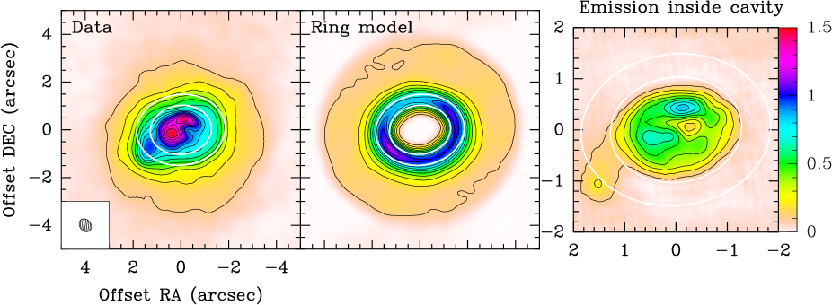
Jy beam^-1 km s^-1

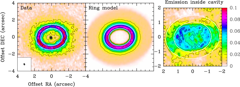
Jy beam^-1 km s^-1

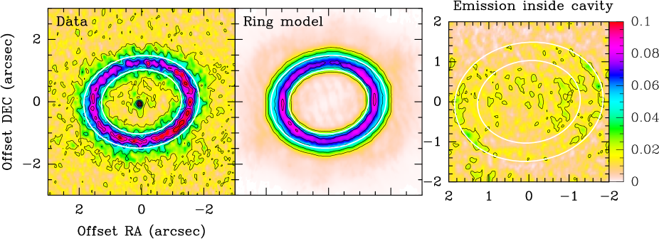
Jy beam^-1 km s^-1

Figure 14: From top to bottom, ${{}^{12}{\rm CO}}$(3–2), ${{}^{13}{\rm CO}}$(3–2) and C¹⁸O(3–2). Left panel: Integrated intensity map. Middle panel: Intensity map of ring and outer disk best-fit model. Right panel: Residual emission inside the cavity (original data minus best-fit model).