Maximum Likelihood Estimation of Spatially Varying Coefficient Models for Large Data with an Application to Real Estate Price Prediction
Abstract
In regression models for spatial data, it is often assumed that the marginal effects of covariates on the response are constant over space. In practice, this assumption might often be questionable. In this article, we show how a Gaussian process-based spatially varying coefficient (SVC) model can be estimated using maximum likelihood estimation (MLE). In addition, we present an approach that scales to large data by applying covariance tapering. We compare our methodology to existing methods such as a Bayesian approach using the stochastic partial differential equation (SPDE) link, geographically weighted regression (GWR), and eigenvector spatial filtering (ESF) in both a simulation study and an application where the goal is to predict prices of real estate apartments in Switzerland. The results from both the simulation study and application show that the MLE approach results in increased predictive accuracy and more precise estimates. Since we use a model-based approach, we can also provide predictive variances. In contrast to existing model-based approaches, our method scales better to data where both the number of spatial points is large and the number of spatially varying covariates is moderately-sized, e.g., above ten.
Keywords: spatial statistics, Gaussian process, covariance tapering, likelihood regularization, real estate mass appraisal
1 Introduction
Over the last years, affordable measuring techniques lead to an abundance of spatial data; not only areal but in particular spatial points data. Often, the data sets contain covariates in addition to the main variable(s) of interest. These are then used in a regression model, where the goal is either predicting the response variable or inferring the relationship between the response variable and the covariates. With further advances to reduce computational cost, we are now able to analyze large spatial data sets and the literature on models and methods on how to do so is extensive. See Cressie (2011) and Heaton et al. (2019) for an overview. However, the vast majority of models assumes that covariate effects are constant over space which is not necessarily plausible.
Spatially varying coefficient (SVC) models allow for marginal effects to be non-stationary over space and thus offer a higher degree of flexibility. At the same time, SVC models have the advantage that they are easily interpretable. Several methodologies and applications with SVC models have been published. To name two, geographically-weighted regression (GWR) by Fotheringham et al. (2002) and a Bayesian framework with SVC processes by Gelfand et al. (2003) are prominent examples. An application that uses both methodologies can be found in Wheeler and Waller (2009) who model crime records in Houston, Texas. In a simulation study Wheeler and Calder (2007) conclude that SVC processes provide more accurate regression coefficient estimates than GWR. A further comparison of GWR and SVC processes is given by Finley (2010) on ecological data. It is shown that SVC processes generally have better predictive performance.
However, when it comes to estimating SVC models on large data, most of the established methodologies run into problems. Currently available implementations of Bayesian approaches such as Gaussian predictive processes presented in Banerjee et al. (2008) or Gaussian Markov random field approximations by Lindgren et al. (2011) are either limited by the number of SVCs within a model or the number of observations. This also holds true for the before mentioned SVC processes by Gelfand et al. (2003). Finally, GWR lacks a statistical sound definition and should be regarded as a purely exploratory tool. Therefore, a geostatistical estimation and prediction method is needed that, on the one hand, can deal with large number of observations and, on the other hand, can be applied to models including many SVCs.
The outline of this article is as follows: In the next section, we introduce the data set and give a first exploratory analysis that motivates the usage of SVC models. In Section 3 we formally define SVC models and give an overview of existing methods. We motivate our approach by listing potential shortcomings of the existing methods. In Section 4 we describe our maximum likelihood estimation (MLE) method in detail. Section 5 compares the existing methods to MLE in a large simulation study on synthetic data. A further comparison on the real data set is given in Section 6. We summarize our findings in Section 7.
2 Data Set
The data set provided by Fahrländer Partner (Zurich, Switzerland) consists of apartment transactions in Switzerland containing the selling price, six covariates and approximate coordinates for each transaction. The goal is to regress the selling price on the given covariates. An overview and description of the data are given in Table 1.
The Swiss banking secrecy prevents disclosing the exact locations of the apartments. That is why all observations are first grouped according to a dense grid consisting of relatively small cells over Switzerland with a higher resolution in densely populated areas. The cell sizes range from to acres ( to ), the median being acres (). Instead of the exact location, we then only observe the centroid of the corresponding cell for every apartment. The easting and northing of these centroids are given in the LV03 coordinate reference system and their corresponding units are meters (Federal Office of Topography swisstopo, 1900).
| Name | Description | Range |
| Price | Transaction amount in Swiss Francs (CHF) | – |
| Area | Area in square meters | 20 – 310 |
| Year of construction | Apartments built before 1920 are set to 1920. | 1920 – 2017 |
| Micro location rating | Rating of the location on small scale, i.e., walking distance (higher meaning better) | 1 – 5 |
| Standard rating | Rating of standard of the apartment (higher meaning better) | 1 – 5 |
| Renovation rating | Need for renovation (lower meaning better) | 0 – 4 |
| Date | Quarter in which the transaction took place | Q3 2015 – Q4 2017 |
| Easting | – | |
| Northing | – |
2.1 Motivation and Exploratory Analysis
In real estate mass appraisal, there are several works that investigate or model non-stationary covariates effects. Gelfand et al. (2003) used a Bayesian SVC model with coefficients defined as Gaussian processes (GP) to model single-family houses in Baton Rouge, Louisiana. A frequently used tool to investigate the hypothesis of SVC in an exploratory manner is geographically weighted regression (GWR). For instance, van Eggermond et al. (2011) and Cao et al. (2019) show that the coefficients of the floor level and the distance to a central business district are spatially varying. We use these findings to motivate a first exploratory analysis of the real estate data set at hand. A visual inspection of the SVCs is challenging since the underlying effects are not directly observable and first require a definition of a regression model.
With the transaction price (price) as a variable of interest we use the area (area), micro location rating (micro), and standard rating (stand) for a simple, first model. Specifically, we natural logarithm transform the price and area variables as one usually does in a hedonic model (Malpezzi, 2008; Wheeler et al., 2014). Using the R package GWmodel by Gollini et al. (2015), the model is fitted on the whole data set and the estimated SVCs are depicted in Figure 1. Due to the heterogeneous distribution of observation locations, we use an adaptive bandwidth which has been estimated using an automated, AIC corrected selection approach (Hurvich et al., 1998).
A visual inspection of the GWR-estimated coefficients indicates that we have indeed spatially varying coefficients. In facet (a) the intercept’s SVC is given. As expected, we see a relatively large variation in the intercept. In addition, the covariates do appear to have spatially varying effects. However, some of the effects are not in line with prior expectation as, for instance, we would expect a higher area effect in city centers. Further, the intercept and the area effect appear negatively correlated. In fact, multicollinearity is a potential drawback of GWR (Wheeler and Tiefelsdorf, 2005; Wheeler and Calder, 2007).
Yet, applications in context of real estate pricing like Cao et al. (2019) as well as Geng et al. (2011) report a substantial increase in by 0.19 and 0.23, respectively, compared to an OLS-based regression. We were able to observe an increase in of similar magnitude when going from an OLS to an GWR estimation. This ambiguity between, on the one hand, the quality of the estimated SVC and, on the other hand, the goodness of fit underlines the need for a statistical sound methodology for SVC models which can be applied to large data.
3 SVC Models
SVC models extend the linear regression model
| (1) |
where are the observations and is the number of coefficients. By allowing the coefficients to vary spatially, the model equation changes to
where denotes the location of observation in a domain . Here, we will work with . The exact specifications for the coefficients have yet to be defined.
3.1 Existing SVC Methods
We will give an overview of the most common methods that allow us to make inference for SVC models.
Geographically Weighted Regression (GWR)
This method is widely used in practice as it is easy to implement and relatively fast in computation. It assumes model equation (1) and estimates the coefficients for each location as a weighted regression specific to that location. GWR is fully described in Fotheringham et al. (2002). As mentioned before, multicollinearity issues with local regressions are raised (Wheeler and Tiefelsdorf, 2005; Wheeler and Calder, 2007), cf. Figure 1. This method is readily available for R (e.g. packages GWmodel by Gollini et al., 2015, spgwr by Bivand and Yu, 2017, and gwrr by Wheeler, 2013) as well as arcGIS (Environmental Systems Research Institute (ESRI), 2020). In its classical form GWR only supports the same bandwidth for all coefficients, that is, the bandwidth is either a fixed distance or adaptive defined by a number of nearest neighbors. Recent works by Fotheringham et al. (2017) and Chen and Mei (2020) present methods to estimate separate bandwidths for each SVC.
Eigenvector Spatial Filtering (ESF)
This method is also known as Moran’s Eigenvector Mapping (MEM) (Griffith, 2011; Dray et al., 2006). In Murakami and Griffith (2015) it has been extended to random effects and thus is now capable of dealing with SVC models. It is readily available in the R packages spmoran (Murakami, 2018) and spatialreg (Bivand and Piras, 2015).
The following methods are based on a model assumption where the SVC is defined with Gaussian processes (GP). That is,
| (2) |
for some choice of covariance function with parameter vector . The covariance function works on the distances between observation locations defined by some norm. Here we use the Euclidean norm . We denote the covariance matrix defined as
| (3) |
One of the most commonly used classes of covariance functions is the Matérn covariance function class. For a marginal variance and a range parameter , we define the Matérn covariance function as
| (4) |
where is the smoothness, is a distance, and is the modified Bessel function of the second kind and order . Coming back to our assumption (2), i.e., that each SVC is modeled by a GP, this implies that each SVC is described by the covariance parameters that consists of a variance and range , while in this paper we assume the smoothness to be known.
Bayesian SVC Processes
Gelfand et al. (2003) introduced a Bayesian SVC model. It allows for prior-dependence of the coefficient processes but assumes an equal range parameter for all coefficients, i.e., . The method is implemented for example in the R package spTDyn (Bakar et al., 2016). However, the package does not scale to large data.
Gaussian Markov Random Fields using an SPDE Link
One can define a Bayesian SVC model using the link between Gaussian Markov random fields (GMRF, see Rue and Held, 2005) and GP via a stochastic partial differential equation (SPDE, see Lindgren et al., 2011). However, this SPDE link only exists for a limited number of Matérn class covariance functions. Estimation can be done using integrated nested Laplacian approximations (INLA) based on Rue et al. (2009) which is available in the R package INLA (www.r-inla.org, Lindgren and Rue, 2015). Due to its widely accommodated models, INLA has become quite popular over the last couple of years and is used in environmental sciences and climatology as it can deal with big data sets. A drawback of INLA is the critical assumption on the number of hyperparameters that one can estimate which should be “small, typically 2 to 5, but not exceeding 20” (Rue et al., 2017) and therefore the number of SVCs in a model is limited.
Remark (SPDE link in INLA).
In the current version of INLA (version 19.09.03), the SPDE link is defined for the fractional operator order . In dimensions, the relation between the fractional operator order and the Matérn smoothness parameter is . In our case () the link exists for Matérn covariance functions with smoothness .
Finally, we want to mention a recent proposal named spatial homogeneity pursuit of regression coefficients by Li and Sang (2019). Spatially clustered coefficient (SCC) models are a sub-class of SVC models. While general SVC models usually assume (smooth) spatial variation, SCCs are defined with constant patches and discontinuities in their coefficients. Li and Sang (2019) use minimum spanning trees – a method from graph theory – to model these SCCs.
3.2 Challenge
Our data model (see below in Section 6.1) contains SVCs and about observations. While the sample size itself poses no computational problems for existing geostatistical approaches for large data, the combination of the sample size and the number of SVCs is challenging. In particular, when applying existing statistical SVC approaches such as in e.g. Gelfand et al. (2003) or Franco-Villoria et al. (2019) to this data, one currently runs into a computational bottleneck. This highlights the need for a statistical methodology that can deal with large data for SVC models.
4 Method: Maximum Likelihood Estimation for SVC Models
In this section, we present the SVC model we use and show how it can be estimated using MLE. We provide novel proposals on how to deal with large data as well as regularization options that help to alleviate correlation among hyper-parameters. Finally, we show how to give predictions once the model has been estimated.
4.1 Gaussian Process-based SVC Model
For each covariate we assume that the associated coefficient is separated into a fixed and a random effect. That is, for some constant and a zero-mean GP with a stationary covariance function similarly to (2), i.e.,
| (5) |
We denote by the data matrix defined as , i.e., the th observation of the th covariate. The fixed effect part is given by , where .
Let be not necessarily distinct observation locations. Using (3) and (5), is normally distributed as
The assumption of mutual prior independence of the GPs, i.e., of , results in having the joint distribution with joint covariance matrix
| (6) |
Further, we denote by a sparse matrix defined as
Using this notation, the random effect part is given by . With the identity matrix , the error term is distributed as and is independent of . In summary, writing the response as an -dimensional vector , we obtain the GP-based SVC model
| (7) |
4.2 Likelihood and Optimization
In the following, we derive the log-likelihood (LL) function for the GP-based SVC model as given in (7). The distribution of the response variable is given by
Given the observed data, the log-likelihood function depends on the covariance parameters as well as the mean parameters :
Maximizing is equivalent to minimizing the function
The solution to the optimization problem
with cannot be computed analytically and one relies on numerical optimization. We use the quasi Newton method "L-BFGS-B" by Byrd et al. (1995) implemented in the R function optim to numerically minimize . This optimization approach repeatedly requires the computation of with updated parameters and subsequently computing both the determinant and the inverse of . Both of these tasks are computationally intensive.
4.2.1 Large Data
It is at this point that the computational burden of constructing and computing its determinant as well as its inverse becomes apparent. Recall that is a matrix of dimension and is of dimension . Using the formal definition of and the sparsity of , one can verify that the construction of alone using the naive matrix multiplication is of run time . A Cholesky-decomposition is then being used to compute both the determinant and the inverse of matrix more efficiently. This however has also runtime .
To reduce the computational load, we will exploit the mutual prior independence of the GPs. We introduce the outer product of a covariate as . This allows us to write using the Hadamard product (also known as the Schur or direct product) as:
| (8) |
Therefore, we do not have to compute the full matrix multiplication and the runtime for the construction of (8) is . To reduce the run time for the Cholesky-decomposition, we use covariance tapering proposed by Furrer et al. (2006). In this approach, we taper the covariance matrices by multiplying them with an appropriate compactly supported correlation matrix, say, , where is the tapering range. Given the underlying covariance functions , without loss of generality, one can choose one corresponding function which is compactly supported on that defines the correlation matrix (Furrer et al., 2006). Then the tapered covariance matrix is sparse with for . Using (8), one can easily verify that
is sparse, too.
4.2.2 ML Estimate Using Direct Optimization Procedure
Using a straightforward optimization approach the ML estimate is defined as
When increasing the number of SVCs , the dimension of parameter space increases and the optimization becomes computationally expensive and numerically unstable. Thus it is crucial to reduce the dimension of the parameter space when working with many SVC. We solve this problem by proposing to optimize the profile likelihood in , which is given by:
where and is the generalized least squares estimator, i.e.,
The ML estimate is given by numerically optimizing the following:
4.2.3 Regularization Using PC Priors
Due to weak identifiability and posterior correlation, the optimization concerning the covariance parameters can be unstable. We want to apply some form of regularization to ensure the numerical optimization problem is well-posed. Recent advances by Simpson et al. (2017) and extensions thereof by Fuglstad et al. (2018) introduced penalizing complexity (PC) priors for Gaussian random fields of Matérn class. We use these PC priors as regularizers to construct a regularized likelihood by extending our pure likelihood or profile likelihood approach from Section 4.2.2, respectively. In the following, we will define the regularized parameter estimate.
In our parametrization of the Matérn covariance function and with , the PC priors for a single GP with range and marginal standard deviation (Fuglstad et al., 2018, Theorem 2.6) take the form
where and are defined by the prior beliefs on the lower tail of the range, , and the upper tail of the standard deviation, , respectively. They are given by and . Under iid assumption on each prior and some initial beliefs this defines the regularized estimate using as:
4.3 Prediction of Coefficient Processes
In the following, we describe how to predict the covariate effects at locations that possibly have not been observed, given estimated parameters . In the classical case of predicting a single GP at spatial points the empirical best linear unbiased predictor (EBLUP) is used (Cressie, 1990). In the case of SVCs, we likewise establish the EBLUP in the following.
We first extend our notation from observed locations to the locations we want to make predictions for, namely . These may or may not include already observed locations. The distributions of and are again normally distributed with respective means and . Estimating the latent coefficient processes is done in a two step approach where we first estimate and then add the mean estimate of . We start by considering the joint distribution
The covariance matrix is defined for locations in an analogous way to (3) and (6), namely and hence
The covariance matrix is given in (8). The cross-covariances matrices and are defined as
where is again defined as (3) and (6), but now with corresponding locations and . Using the conditional distribution and plugging in one receives the EBLUP for SVC as
and therefore . One can then use corresponding data and at locations to get predictions for . Predictive variances of such are derived in a similar way as above and given by the diagonal of .
4.4 R package varycoef
The MLE described in this section is implemented in the R package varycoef (Dambon et al., 2020). It utilizes parallel computing as well as sparse matrix representation and computation for numeric optimization procedures (Gerber and Furrer, 2019; Furrer and Sain, 2010). This package is used throughout this work whenever the MLE approach is mentioned. We indicate the usage of our method and the R package varycoef on GP-based SVC models by the abbreviation MLE with suffixes.
5 Simulation Study
This and the next section are designated to compare existing and our proposed methods in regard to parameter estimation and prediction accuracy. From Section 3.1, we exclude the Bayesian SVC processes method since it does not scale to large data. Further, since SCC and smooth SVC models are inherently different, we exclude the spatial homogeneity pursuit approach, too.
5.1 Setup
In order to empirically validate our method and to compare it to existing methods, we define the following simulation setup. We simulate times a GP with varying numbers of SVCs and sample sizes . Latter is defined by a positive integer such that is the number of data points and locations which are sampled from a perturbed grid (Furrer et al., 2016).
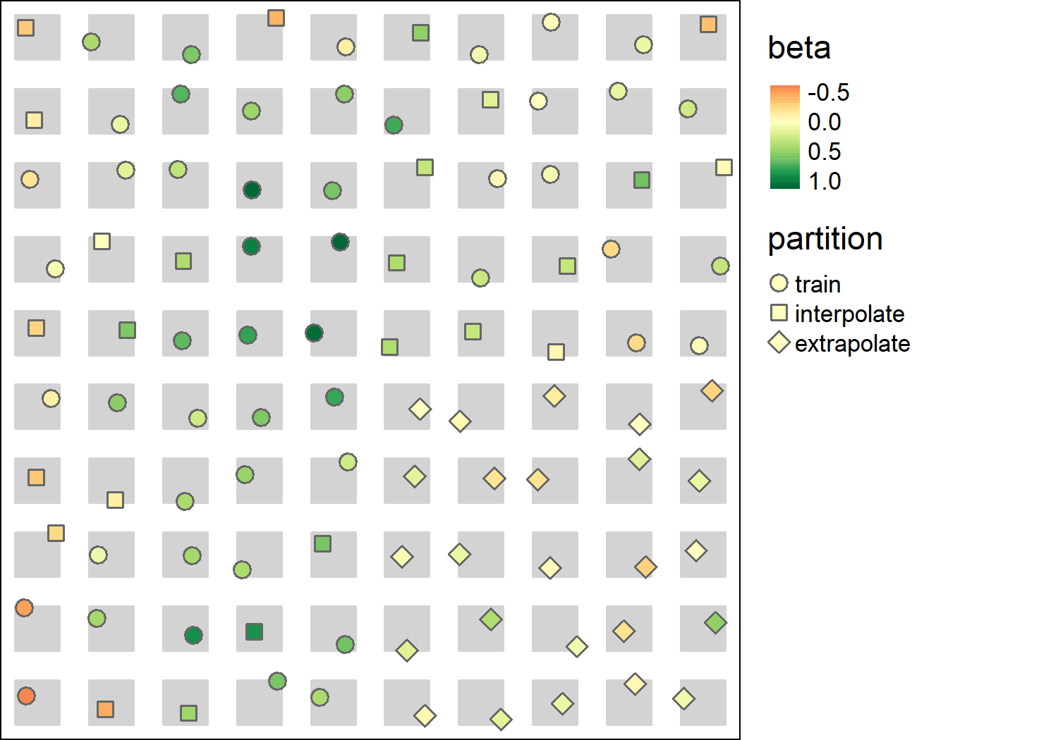
A perturbed grid consists of unit squares. For each , we uniformly draw a single location from a square , where restricts a unit square area by an outer margin. Finally, we standardize the locations by such that the total domain of a perturbed grid is contained in the unit square. Thus, we receive the sample locations . An example is given in Figure 2.
At these locations the SVCs, the error term , and the data are sampled and we compute the response . We set which allows us to model a spatially varying intercept. The remaining data of is sampled from a standard-normal distribution for coefficients .
The data is then divided into three disjoint folds, (i) a training data set , (ii) a test data set for interpolation , and (iii) a test data set for extrapolation . The unit square is partitioned into four quadrants. The lower right quadrant is an extrapolation test set and contains of the data. In the other quadrants, of the data is randomly assigned as interpolation test set. On the rest () of the data, the model is being estimated. Thus, we have a partition:
In total, there are three simulation settings which differ in the number of total sampled points and SVCs and five methods for SVC modeling, see Table 2 for an overview. For our proposed methodology, we maximize the regularized profile likelihood and label it as MLE.r. The SPDE method has been implemented with the R package INLA (Lindgren and Rue, 2015) and uses the same PC priors as MLE.r, namely and . The methods ESF and GWR are implemented with the R packages spmoran (Murakami, 2018) and GWmodel (Gollini et al., 2015), respectively. For GWR, we use the same bandwidth for all covariates as the prediction function does not support covariate specific bandwidths. The bandwidths are estimated using a cross validation and are not adaptive, i.e., they are defined as fixed distances due to the regular structure of the perturbed grid. The superscript tap in Table 2 indicates covariance tapering for MLE, since Simulation 2 has the most observations. The taper range is . Due to the number of SVCs, the SPDE method cannot be applied on Simulation 2, hence the cross marks in Table 2.
| Simulations | ||||
| 1 | 2 | 3 | ||
| 3 | 3 | 10 | ||
| Methods | ||||
| MLE.r | ||||
| SPDE | ✗ | |||
| ESF | ||||
| GWR | ||||
In each repetition and for each method , we calculate the RMSE between the estimated SVC and the true SVC in each fold
Analogously, we calculate the RMSE for the response. Thus, we have:
| (9) | ||||
| (10) |
In all of our simulation studies we assume the type of covariance function to be known, which is why we have to define it here. Since we expect in most of our applications the fields to be not too smooth, we follow the recommendation of Stein (1999) and use exponential covariance functions. The exponential covariance function is a special case of the Matérn class covariance functions with smoothness parameter , cf. (4). Thus, we have
5.2 Results
5.2.1 Simulation 1: Base Setup
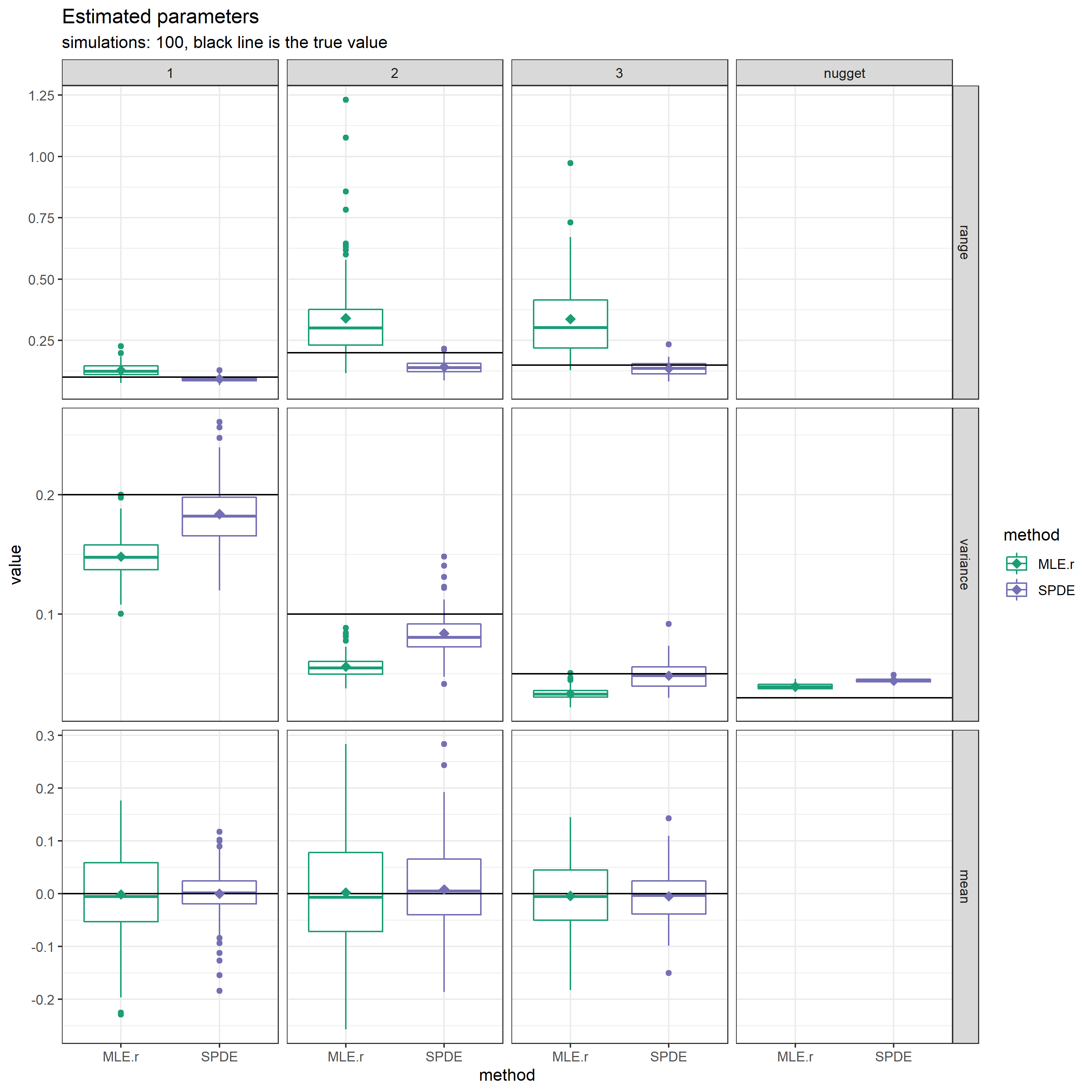
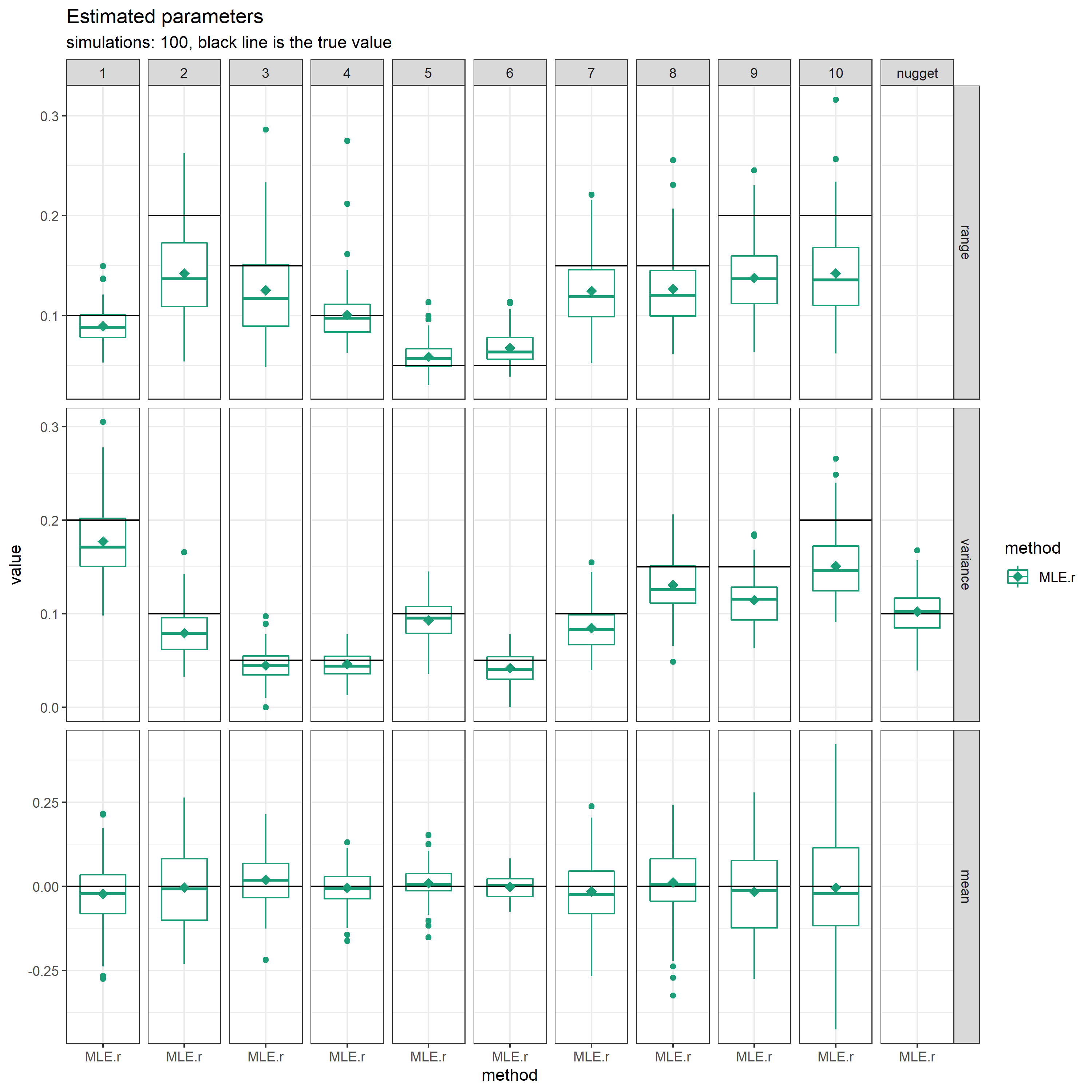
The base simulation setup samples from a perturbed grid with SVCs. The parameters of the true model are provided in Table 3. The results of the parameter estimation which is available for the methods MLE.r and SPDE are given in Figure 3. The results are quite similar. While the SPDE’s estimates of the range usually are higher than those of MLE.r, SPDE overestimates the nugget variance. Regarding the mean effects, SPDE appears to estimate mean effects with more precision.
| Effects | |||
| Parameters | 1 | 2 | 3 |
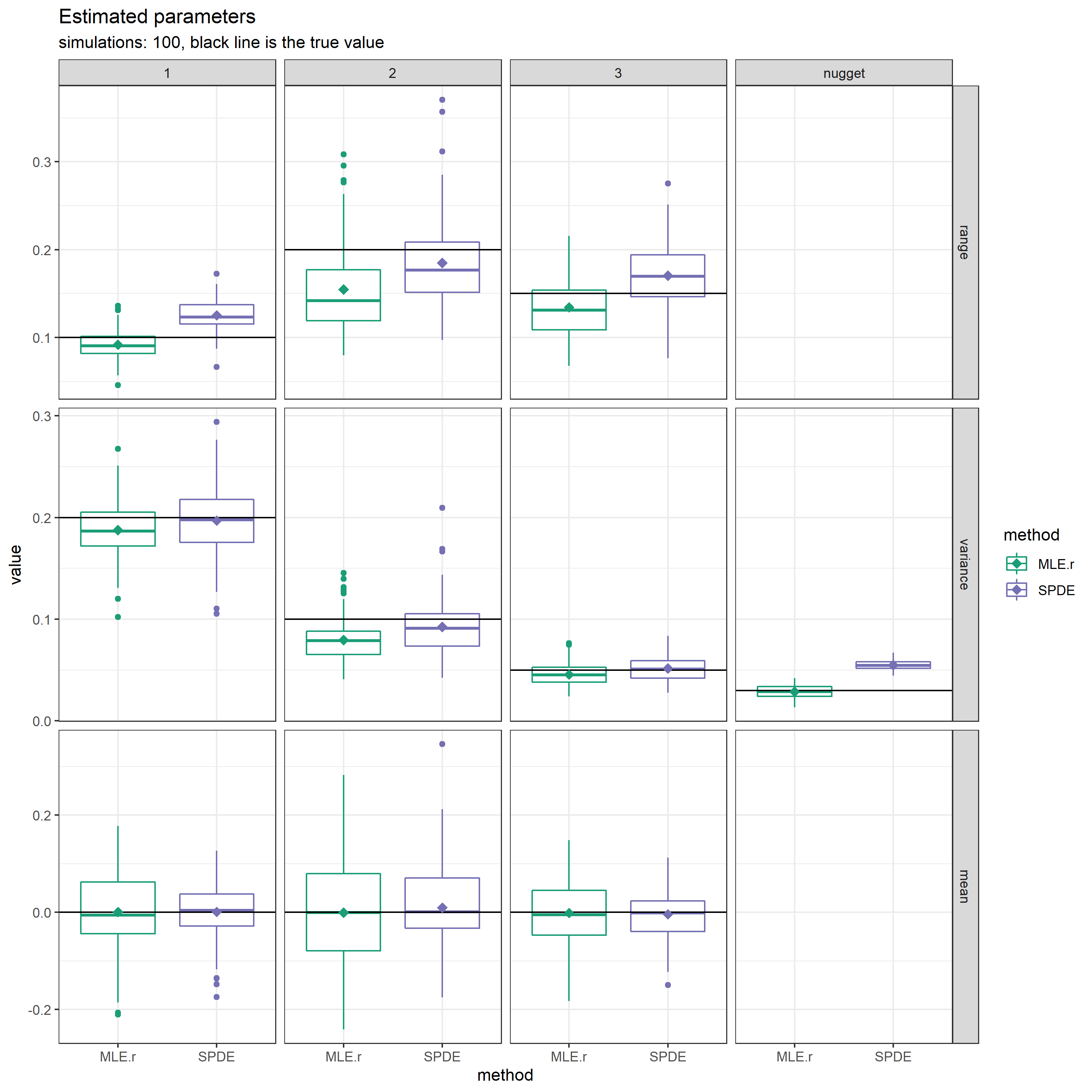
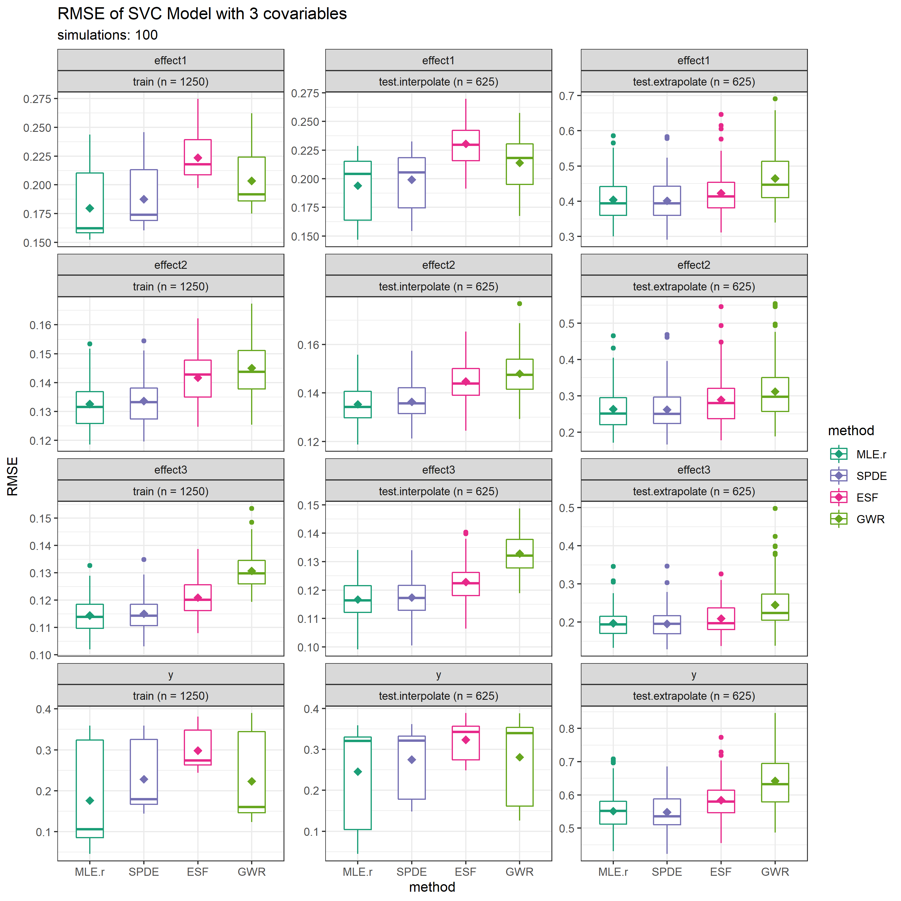
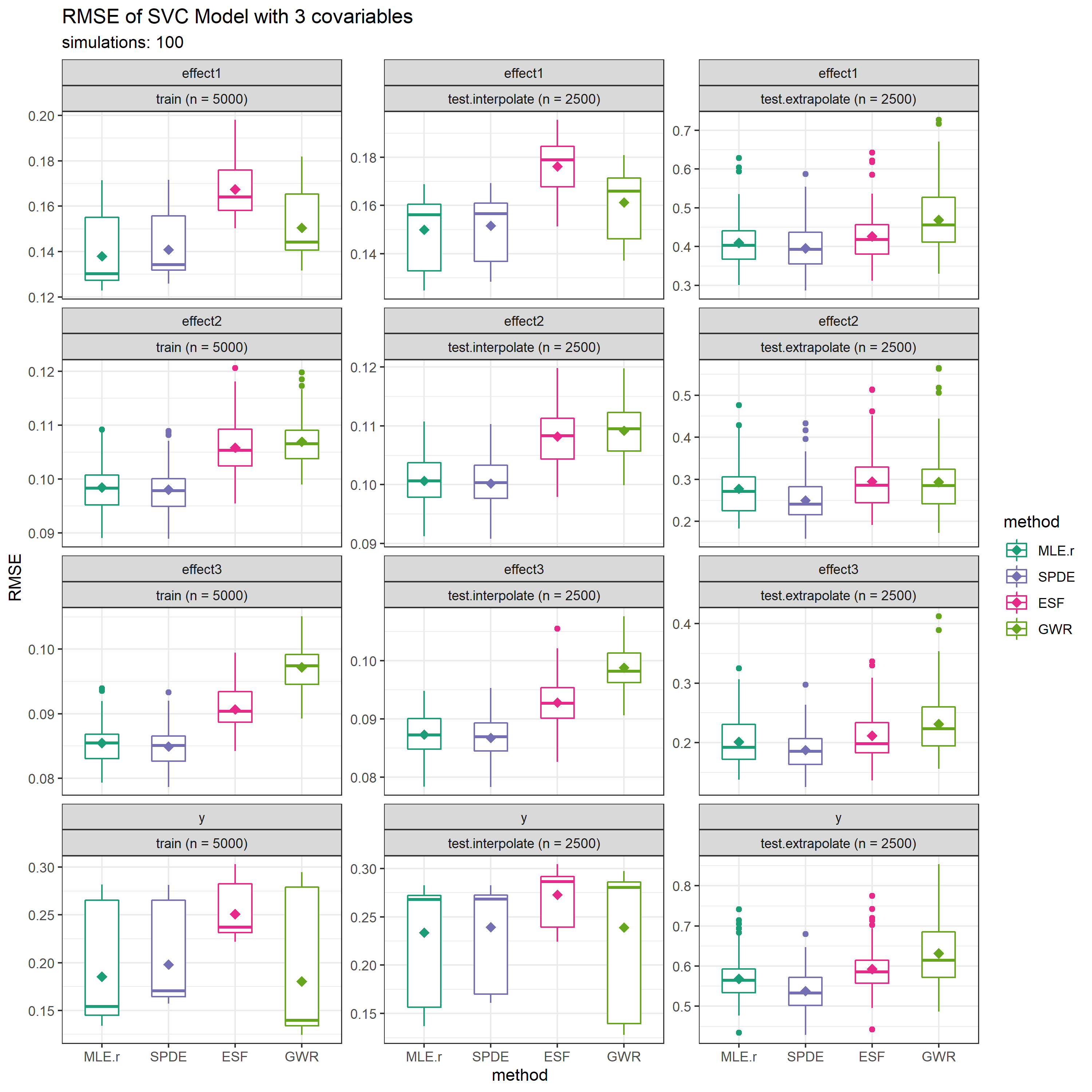
The results for the RMSEs are depicted as box plots in Figure 4 for all 100 repetitions within the simulation. The RMSE as given in (9) reveals some interesting insights. MLE.r consistently gives some of the best training and prediction results. It is closely followed by SPDE. ESF and GWR clearly have lower accuracy. Spatial extrapolation as depicted in the last column is much more difficult for all methods. But, model-based approaches perform better than the non-model based alternatives. The results for SVC’s RMSE probably translate to the results for the response’s RMSE, where it appears that the intercept is the main driver. Overall, MLE.r has the highest in-sample and out-of-sample predictive accuracy, closely followed by SPDE. ESF and GWR have lower predictive accuracy.
5.2.2 Simulation 2: Number of Observations is
Simulation 2 has the same underlying true model to simulate the data from, cf. Table 3, but using a data set with observations. In order to allow our method to scale to data sets with a large , we introduced covariance tapering (Furrer et al., 2006) in both MLE without and with regularization. With the introduction of a tapering range, which in this simulation study was set to , the covariance matrices become sparse. While this has a positive impact on computation time, it results in biased estimates for the covariance parameters. Due to tapering, the ranges were overestimated by MLE.r, whilst all variances of the SVCs were underestimated. SPDE performed very similarly as in Simulation 1, cf. Figure 5.
Further, we compute the RMSE as given in (9) and (10). The results are depicted in Appendix A.1. They are very similar to what we observed in Simulation 1 with Figure 4. The main difference that we can see is that the GWR has a broad range of quality when estimating and predicting the response, while clearly falling behind when modeling the SVCs.
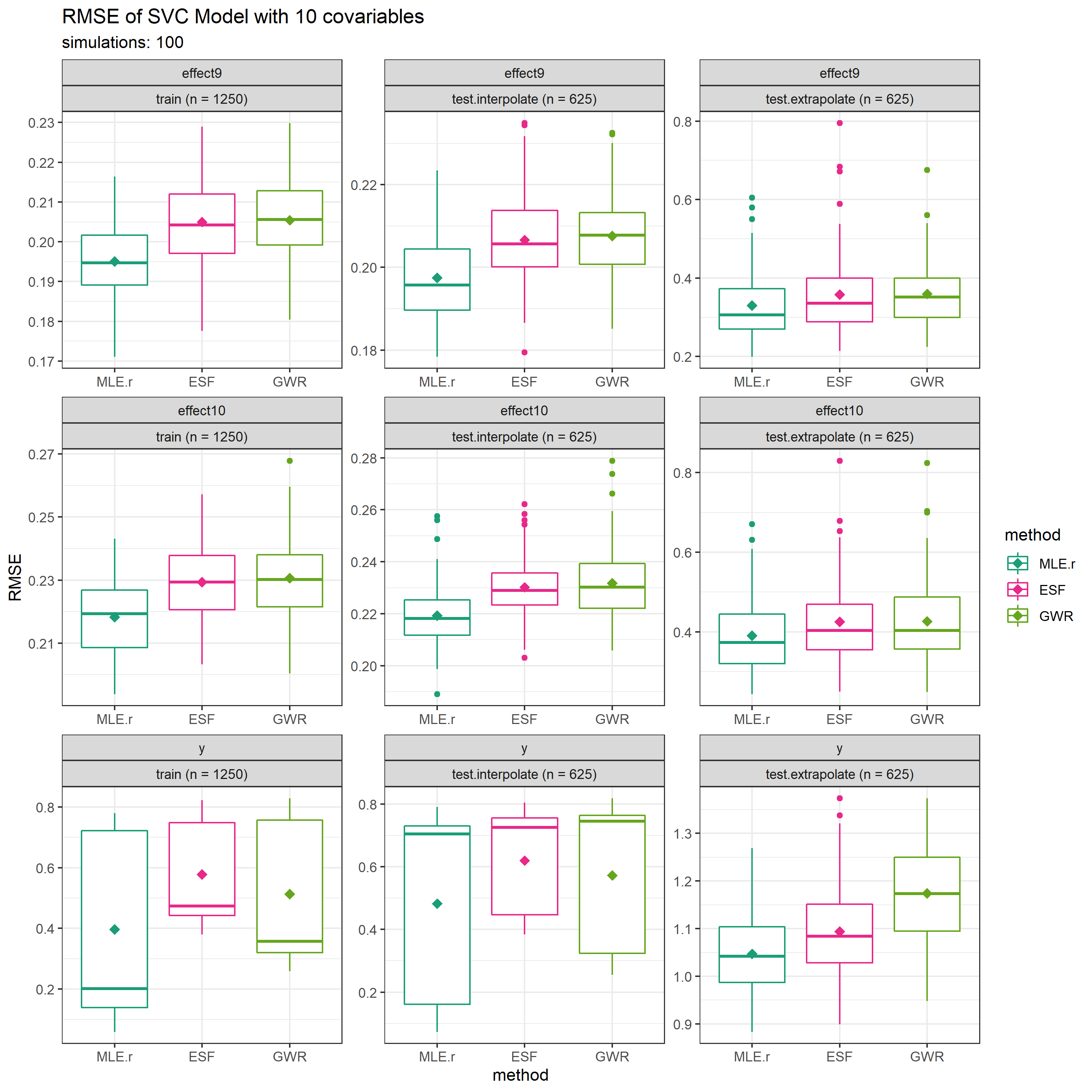
5.2.3 Simulation 3: Number of SVCs is
In this simulation, we have SVCs sampled from the model with the true parameters as defined in Table 4. We cannot run SPDE due to too many SVCs. Thus, MLE.r is the only method with which we are able to estimate the parameters. The empirical results show that our ML-estimator yields unbiased results, which qualitatively are close to the results of MLE given in Figure 3. In predictive performance measured by the RMSE, MLE.r surpasses both ESF and GWR. All of the results are depicted in Appendix A.2.
| Effects | ||||||||||
| Parameters | 1 | 2 | 3 | 4 | 5 | 6 | 7 | 8 | 9 | 10 |
5.2.4 Summary
Over all simulations, our proposed MLE approach is competitive with other methodologies for SVC modeling. In particular, the parameter estimation is unbiased when not using tapering and scales to models with a moderate number of SVCs. Further, the modeling and predicting capabilities as measured using the RMSE are among the best.
In the following, we also report computation time. The simulations were run on a server with 8 Intel Xeon 10 core E7-2850 with 2.0 GHz for a total of 80 threads and 2 TB of memory under Ubuntu OS. Computations run time was measured for each repetition and method run. The results are given in Table 5.
| Methods | ||||
| Simulations | MLE.r | SPDE | ESF | GWR |
| 1 | ||||
| 2 | ||||
| 3 | ||||
Overall, the results are in line with our expectations. Model-based estimation and prediction approaches are much slower than non-model-based procedures. While increasing the number of SVCs , the computation time only increases slightly for all methods, the increase of computation time is much more pronounced when increasing the number of observations. Note that the computational time for MLE.r in the large case depends on the amount of tapering. Using a smaller taper range would decrease the computational time.
6 Application: Real Estate Pricing
In prior consultation with real estate experts at Fahrländer Partner, real estate mass appraisal will be done on a model fitted on transactions from six consecutive quarters using (transformed or scaled) covariates given in Table 1. Predictions are then given for the following seventh quarter. The rationale behind this setup is to account for a time trend.
The focus of this application lies – like in previous simulation studies – on two aspects. First, we will compare and analyze the outputs of ML-estimated GP-based models with respect to parameter estimation and interpretation of the estimated SVCs (Section 6.3). Second, we will expand this frame work in order to compare the predictive performance of the different methods (Section 6.4). We use a moving window validation. That is, we divide the data set into 4 folds (). Each fold consists of data from 6 consecutive quarters which are used to estimate the model and a following seventh quarter which is used for evaluating the predictive accuracy. A visualization of the moving windows is given in Table 6.
| 2015 | 2016 | 2017 | ||||||||
| Folds | Q3 | Q4 | Q1 | Q2 | Q3 | Q4 | Q1 | Q2 | Q3 | Q4 |
| 1 | ||||||||||
| 2 | ||||||||||
| 3 | ||||||||||
| 4 | ||||||||||
6.1 SVC Model for Real Estate Pricing
We extend the previous simple model used in Section 2.1 and add i) a standardized age defined with the year of construction yoc, ii) as one expects a quadratic age effect in hedonic models in Europe (Brunauer et al., 2010; Fahrländer, 2006), iii) the renovation rating renov, and iv) a dummy variable constructed from the quarter of transaction. Latter is defined as
This is to differentiate the most recent transactions from the rest of the training set in order to account for the temporal trend and should enhance the predictive performance. In summary, we will obtain the following model with SVCs:
| (11) | ||||||||
where the locations are given in transformed LV03 coordinates. More precisely, the easting (LV03x) and northing (LV03y) are now centered on the origin and transformed to kilometers, i.e.
This procedure increases numerical stability while still providing interpretability of distances.
6.2 MLE Specifications
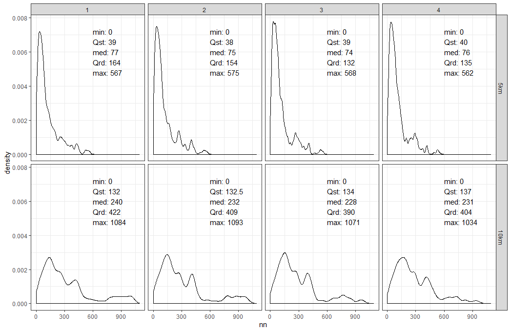
The underlying SVC model is (11) where – as in the simulation study – we assume exponential covariance functions for all GPs modeling the SVCs. Further, we use regularization for the ranges and variances, i.e. and in corresponding units. Due to the large number of observations, we apply covariance tapering. The taper range was set to kilometers, as at least half of the observations of the training data have 74 or more neighbors within their taper range, cf. Figure 13 in Appendix B. To stay consistent with the definition in the simulation study, we use the same label MLE.r for this model and above described method specifications.
6.3 Model Output and Interpretation
We start with a single MLE.r model output. It was estimated on , cf. Table 6. To provide a reference, we compare it to a classical geostatistical model. That is, the underlying model only contains one GP for the intercept, while all other covariates enter the model only as fixed effects. Though the models differ, we use the same methodology and specification as described for the GP-based SVC model, i.e., profile likelihood optimization using the same regularization and tapering range as previously described. We label it MLE.geo.
The estimated parameters of both the MLE.r and MLE.geo models are given in Table 7. We note that the estimated mean effects are very similar. Moving to the covariance parameters of the SVC model, note that the estimates are indeed very different for ranges and variances. The bias due to covariance tapering is notable in the range parameters . The four range parameters exceeding the taper range of 5 kilometers would have an effective range of with an exponential covariance function. This would translate to effective ranges of – in some cases – well over 200 kilometers, and therefore almost as large as the dimensions of Switzerland. In the context of real estate pricing this would not make sense. But we have to recall that due to tapering all covariance functions are compactly supported on .
| MLE.r | MLE.geo | ||||||
| SVCs | |||||||
| 1 | Intercept | ||||||
| 2 | log area | – | – | ||||
| 3 | Z.age | – | – | ||||
| 4 | – | – | |||||
| 5 | stand | – | – | ||||
| 6 | micro | – | – | ||||
| 7 | renov | – | – | ||||
| 8 | – | – | |||||
| Nugget | – | – | – | – | |||
Further, we notice the relatively large estimates for the variance in the intercept as well as the nugget in the SVC model. Although the covariates are not standardized, they do have a similar range of values that they can take, cf. ranges in Table 1. This leads us to believe that, on the one hand, the mean pricing level is one of the dominant factors when it comes to real estate pricing. On the other hand, the large nugget variance suggests that there exists a high residual variability of apartments within the data set.
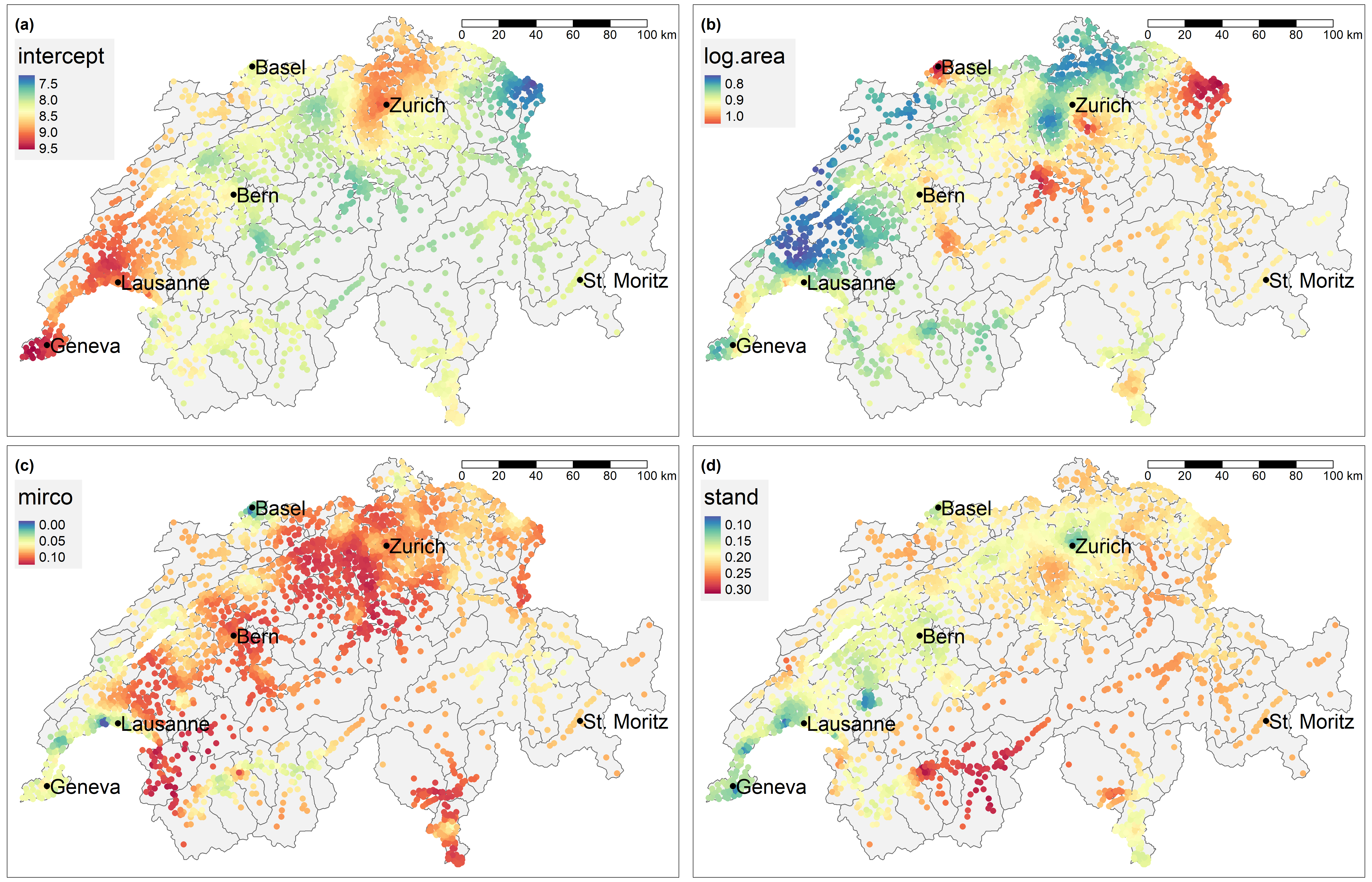
We will now take a look at the visualized SVCs as in Figure 1, i.e., the intercept, log area, and the ratings of micro locations and standard micro and stand, respectively. These are also the ones with the largest estimated ranges suggesting that the spatial structure will be most prominent in these SVCs. All other covariates SVCs are given in Appendix C.
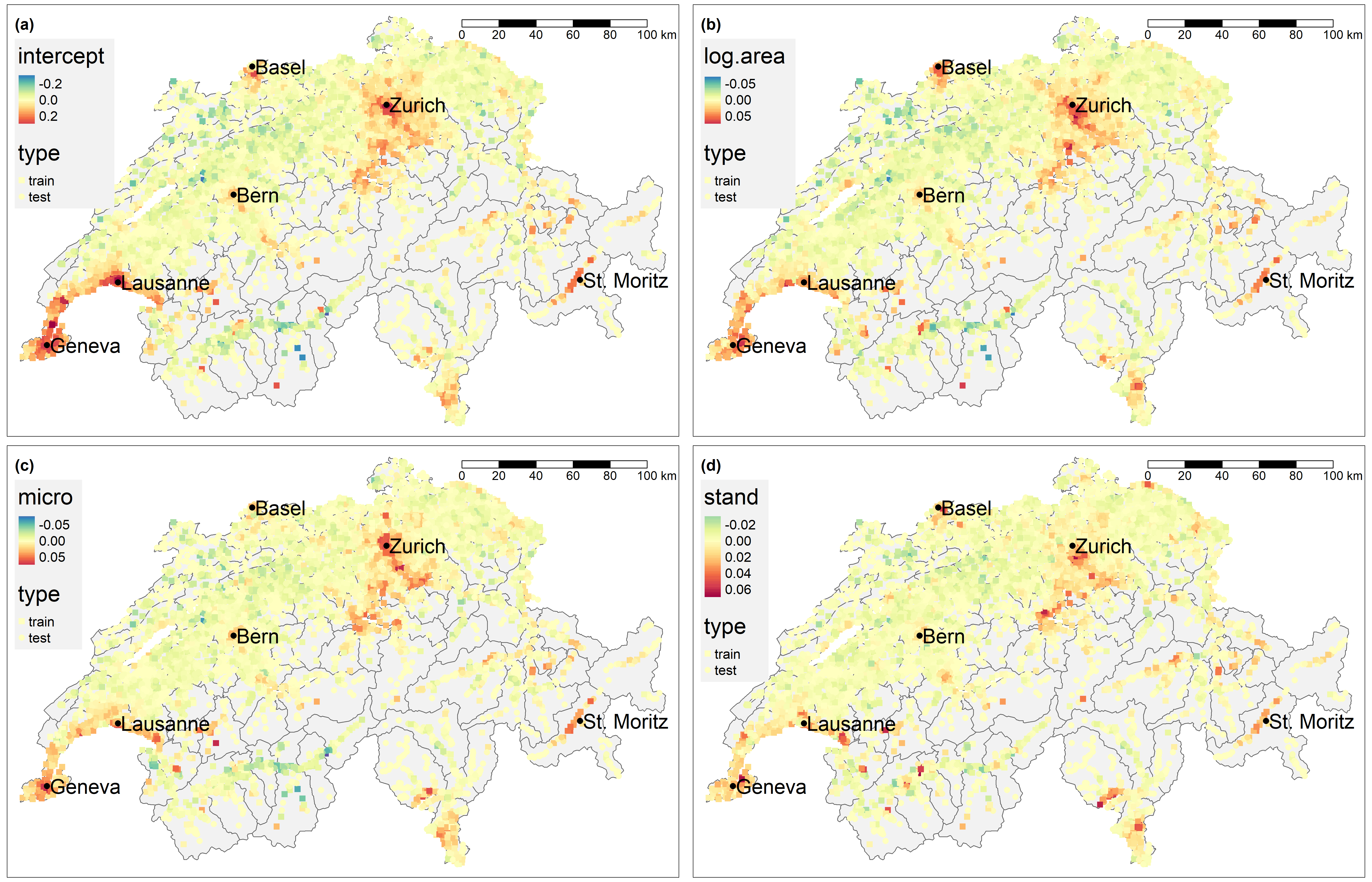
Recall that due to their definition as zero-mean GPs, the interpretation of ML-estimated SVCs is different than what we saw in Figure 1. For GWR the mean effect of each SVC was included. Therefore, one has to interpret Figure 6 as deviations from mean effects, which are given in Table 7. For the intercept depicted in Figure 6(a), one can clearly see that the mean apartment prices are highest in the agglomerations of Zurich, Geneva, and Basel as well as the alpine resort Saint Moritz. The mean prices are also higher along the shore line of Lake Geneva starting from the city of Geneva and reaching as far as Lausanne. More rural areas such as between Basel and Bern or in the alpine regions south of Bern have lower mean apartment prices. Qualitatively, the overall picture does not change too much when comparing to Figure 6(b) to (d), i.e., the SVCs of log area, micro, and stand. There are however some differences.
For example, along the shore line of Lake Geneva, the effect of micro and stand is smaller compared to the city center of Geneva. However, the mean prizes in Lausanne are relatively high. This suggests that the standard or micro location rating of an apartment in Lausanne is not as important as its location.
Overall, the quality of the ML-estimated SVCs as displayed in Figure 6 seems more plausible and in line with expert knowledge compared to GWR-estimated SVCs in Figure 1. There are no highly questionable deviations as seen in Figure 1(a) and (b). Also the estimated ranges vary between the SVCs. For instance, the SVCs for micro location and standard rating are much more locally pronounced as compared to the intercept and log area.
6.4 Predictive Performance
In this last part of the real estate application, we evaluate the predictive performance of MLE.r, MLE.geo, GWR and ESF. The SPDE method cannot be considered as there are too many hyper parameters for INLA. In order to compare the predictive performance of the different approaches, we use the moving window validation setting introduced in Table 6. For each fold and method , we fit a model on the data and then make predictions for out-of-sample observations . For GWR, this includes an adaptive bandwidth selection as described in Figure 1 for each fold . Thus, we have . By doing so, we can compute the prediction errors and the RMSE as follows:
| (12) | ||||
| (13) |
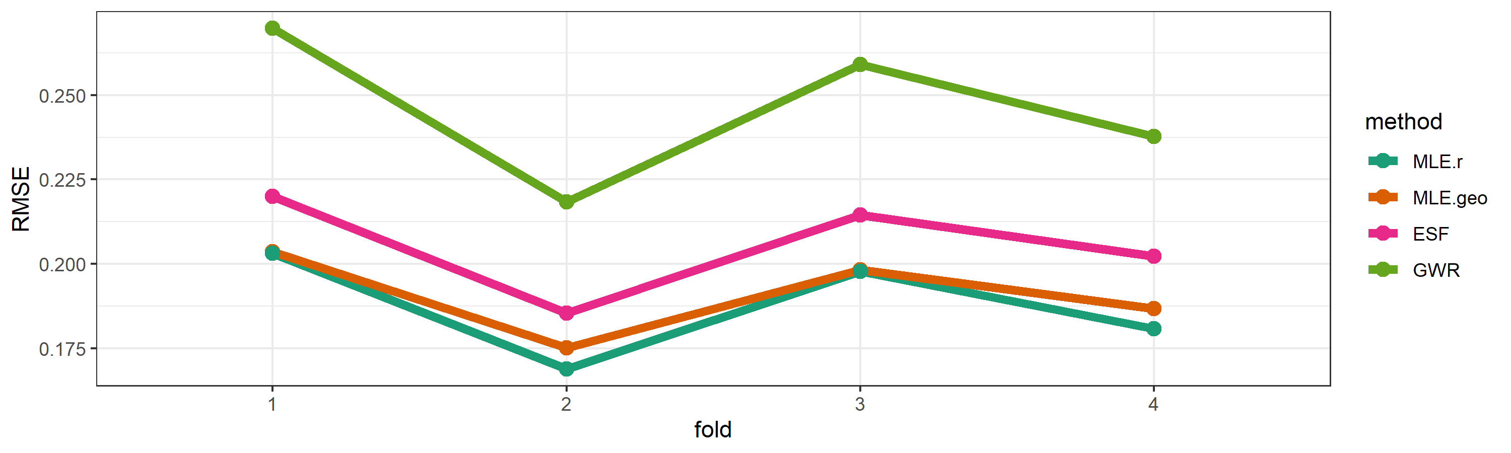
We depict the results for the RMSE in Figure 7. We find that the GP-based SVC model performs best. Further, it shows that model-based methods outperform ESF and especially GWR throughout all folds. The differences between both MLE for an SVC and a geostatistical model are relatively small.
In the following, we investigate whether the differences are significant by using a mixed effect model describing the RMSE as defined in (13). The reference method is the MLE-based SVC model MLE.r defined as the intercept . For the methods MLE.geo, ESF, and GWR we include deviations from the reference level . Further, we include a random effect for the fold, i.e. a temporal effect, with iid as well as an iid noise variable . The model describing the RMSE is therefore given by
| (14) |
The model has been estimated using the R package lmerTest (Kuznetsova et al., 2017) and the main results are given in Table 8, while the whole analysis can be found in the supplementary material. They confirm the conclusions drawn from Figure 7. In particular, the RMSE for ESF and GWR is significantly higher than for MLE methods. However, the difference in RMSE between MLE.r and MLE.geo is not significant at 5% level.
6.4.1 Detailed Prediction Error Analysis
In the following, we perform a detailed prediction error analysis that takes into account that errors of the different methods for the same apartments are correlated. Similarly to model (14), we analyze the prediction errors as defined in (12) using a mixed effect model. The independent variables contain a fixed effect for each method which we define with . Further, notice that we have repeated measures, since every apartment has been predicted by each method. We can account for this by an iid random effect for the different apartments. Finally, we add iid for the noise with distinct standard deviation for each method. The underlying mixed effect model is
| (15) |
When estimating the model, we expect the estimates of to be near 0, since the predictions should be unbiased. Further, the main focus should be on the estimated standard deviations of the noise, as they indicate the uncertainty of the corresponding methods. The estimation was conducted using the R package nlme (Pinheiro et al., 2018) and the main results are given in Table 8. The estimated fixed effects are in fact close to 0, the estimated standard deviations are increasing throughout the methods indicating a higher precision for predictions under MLE. The standard deviation for the apartment-specific random effect was estimated with . This again indicates the high variability of apartments that the models have to predict. The full analysis can be found in the supplementary material.
| Model (14) | Model (15) | |||
| Methods | -value | |||
| MLE.r | – | – | 0.0037 (0.0018) | 0.0465 |
| MLE.geo | 0.0032 (0.0032) | 0.3357 | 0.0014 (0.0018) | 0.0516 |
| ESF | 0.0179 (0.0032) | 0.0003 | 0.0045 (0.0021) | 0.1202 |
| GWR | 0.0586 (0.0032) | 0.0000 | 0.0445 (0.0023) | 0.1674 |
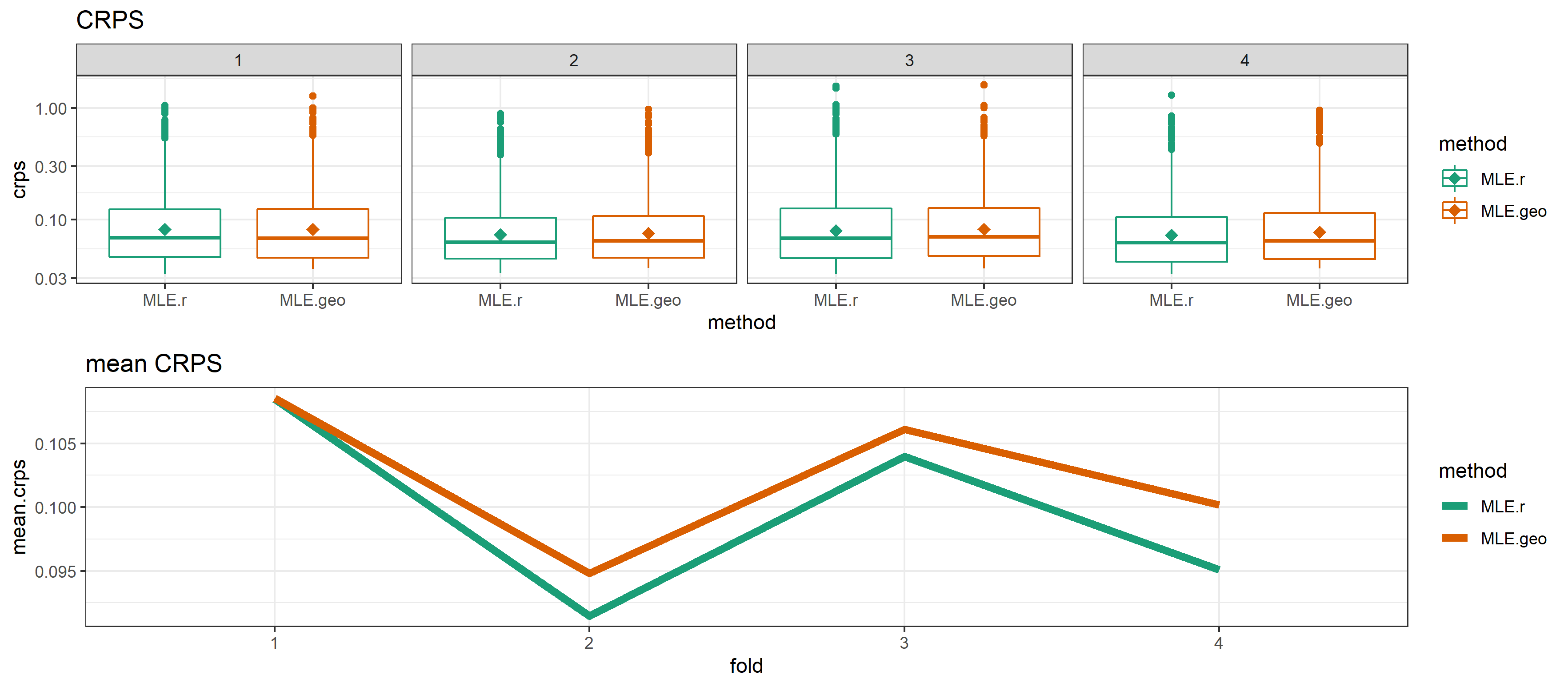
6.4.2 Probabilistic Predictions
The GP-based geostatistical and SVC model allow us to provide a a predictive distribution instead of merely a point prediction. We use the continuous ranked probability score (CRPS) proposed by Gneiting and Raftery (2007) to assess the accuracy of the predictive distributions. The results are depicted in Figure 8. Compared to Figure 7 with the RMSE, one can observe that the SVC model has an advantage with respect to quantifying the uncertainty over the geostatistical model with only having spatially varying intercept.
6.4.3 Summary Predictive Performance
The extensive investigation of predictive performance in the real estate application showed that the MLE method applied on the GP-based models performs considerably better than the other methods, while offering the possibility to quantify the uncertainty of predictions. When it comes to the comparison of the geostatistical to the SVC model, the differences are more subtle. In our application, the gain by modeling and predicting the apartment prices with SVC models instead of geostatistical models is small, whereas the SVC model quantifies uncertainties better. As mentioned in Section 6.3, this might be due to the location as a dominant factor in real estate mass appraisal.
7 Conclusion
In this paper, we presented an MLE approach for GP-based SVC models. We empirically validated our approach against other, existing methods for SVC models. This has been done in a simulation study as well as an application with real estate data. To the best of our knowledge, our proposed methodology is the only implemented and currently available method to estimate and make predictions for GP-based SVC models in context of large data where both the sample size and the number of SVCs are large.
Parameter estimations were shown to be accurate and unbiased when not applying covariance tapering. The predictive performance is in both the simulation study as well as the application among the best. In contrast to not model based approaches such as GWR and ESF it is able to quantify uncertainty by giving predictive variance.
All GPs were defined by exponential covariance functions and based on Euclidean distances in a two-dimensional domain. However, our proposed method can easily be extended to allow GP-based SVC models defined by individual, non-stationary (anisotropic) covariance functions using other norms on higher dimensional domains with . Here, MLE could even be augmented to estimate, say, the smoothness.
We make some final remarks on future work: First and foremost, it would be greatly appreciated to see further comparisons of existing SVC methods on other data sets to see how the predictive performance compares.
Further, multicollinearity issues with GWR have been raised and one should also investigate if this translates to our methodology. This is in accordance with some SVC selection method that has to be developed to check whether a coefficient is constant or spatially varying.
Acknowledgment
We gratefully acknowledge the support by the Swiss Innovation Agency Innosuisse, project number 28408.1 PFES-ES. We would like to thank Leonhard Held for his helpful comments on this paper. We also would like to thank Manuel Lehner and Jaron Schlesinger from Fahrländer Partner for their valuable input towards the application with real estate appraisal.
We appreciate the constructive feedback by the anonymous reviewers and the editor which improved the quality of this work.
Supplementary Material
The code for computation is available online under https://git.math.uzh.ch/jdambo/open-access-svc-paper. Additionally, we provide the following supplementary material.
- Appendix:
-
Additional results and figures. (PDF)
- R package varycoef:
-
R package by Dambon et al. (2020) containing the routines of the MLE method for SVC models described in this article. (GNU zipped tar file)
References
- Bakar et al. (2016) Bakar, K. S., P. Kokic, and H. Jin (2016). Hierarchical Spatially Varying Coefficient and Temporal Dynamic Process Models Using spTDyn. Journal of Statistical Computation and Simulation 86(4), 820–840.
- Banerjee et al. (2008) Banerjee, S., A. E. Gelfand, A. O. Finley, and H. Sang (2008). Gaussian Predictive Process Models for Large Spatial Data Sets. Journal of the Royal Statistical Society: Series B (Statistical Methodology) 70(4), 825–848.
- Bivand and Yu (2017) Bivand, R. and D. Yu (2017). spgwr: Geographically Weighted Regression. R Package Version 0.6-32, https://CRAN.R-project.org/package=spgwr.
- Bivand and Piras (2015) Bivand, R. S. and G. Piras (2015). Comparing Implementations of Estimation Methods for Spatial Econometrics. Journal of Statistical Software 63(18), 1–36.
- Brunauer et al. (2010) Brunauer, W. A., S. Lang, P. Wechselberger, and S. Bienert (2010). Additive Hedonic Regression Models with Spatial Scaling Factors: An Application for Rents in Vienna. The Journal of Real Estate Finance and Economics 41(4), 390–411.
- Byrd et al. (1995) Byrd, R. H., P. Lu, J. Nocedal, and C. Zhu (1995). A Limited Memory Algorithm for Bound Constrained Optimization. SIAM Journal on Scientific Computing 16(5), 1190–1208.
- Cao et al. (2019) Cao, K., M. Diao, and B. Wu (2019). A Big Data–Based Geographically Weighted Regression Model for Public Housing Prices: A Case Study in Singapore. Annals of the American Association of Geographers 109(1), 173–186.
- Chen and Mei (2020) Chen, F. and C.-L. Mei (2020). Scale-adaptive Estimation of Mixed Geographically Weighted Regression Models. Economic Modelling.
- Cressie (1990) Cressie, N. (1990). The Origins of Kriging. Mathematical Geology 22(3), 239–252.
- Cressie (2011) Cressie, N. (2011). Statistics for Spatio-Temporal Data. Wiley Series in Probability and Statistics. Hoboken, N.J: Wiley.
- Dambon et al. (2020) Dambon, J. A., F. Sigrist, and R. Furrer (2020). varycoef: Varying Coefficients. R Package Version 0.2.12, https://cran.r-project.org/package=varycoef.
- Dray et al. (2006) Dray, S., P. Legendre, and P. R. Peres-Neto (2006). Spatial Modelling: A Comprehensive Framework for Principal Coordinate Analysis of Neighbour Matrices (PCNM). Ecological Modelling 196(3), 483 – 493.
- Environmental Systems Research Institute (ESRI) (2020) Environmental Systems Research Institute (ESRI) (2020). ArcGIS Pro. http://pro.arcgis.com/en/pro-app/tool-reference/spatial-statistics/geographicallyweightedregression.htm.
- Fahrländer (2006) Fahrländer, S. S. (2006). Semiparametric Construction of Spatial Generalized Hedonic Models for Private Properties. Swiss Journal of Economics and Statistics 142(4), 501–528.
- Federal Office of Topography swisstopo (1900) Federal Office of Topography swisstopo (1900). LV03. https://www.swisstopo.admin.ch/en/knowledge-facts/surveying-geodesy/reference-frames/local/lv03.html.
- Finley (2010) Finley, A. O. (2010). Comparing Spatially-Varying Coefficients Models for Analysis of Ecological Data with Non-Stationary and Anisotropic Residual Dependence. Methods in Ecology and Evolution 2(2), 143–154.
- Fotheringham et al. (2002) Fotheringham, A. S., C. Brunsdon, and M. Charlton (2002). Geographically Weighted Regression: The Analysis of Spatially Varying Relationships. Chichester: Wiley.
- Fotheringham et al. (2017) Fotheringham, A. S., W. Yang, and W. Kang (2017). Multiscale Geographically Weighted Regression (MGWR). Annals of the American Association of Geographers 107(6), 1247–1265.
- Franco-Villoria et al. (2019) Franco-Villoria, M., M. Ventrucci, and H. Rue (2019). A Unified View on Bayesian Varying Coefficient Models. Electronic Journal of Statistics 13(2), 5334–5359.
- Fuglstad et al. (2018) Fuglstad, G.-A., D. P. Simpson, F. K. Lindgren, and H. Rue (2018). Constructing Priors that Penalize the Complexity of Gaussian Random Fields. Journal of the American Statistical Association 114(525), 445–452.
- Furrer et al. (2016) Furrer, R., F. Bachoc, and J. Du (2016). Asymptotic Properties of Multivariate Tapering for Estimation and Prediction. Journal of Multivariate Analysis 149, 177–191.
- Furrer et al. (2006) Furrer, R., M. G. Genton, and D. W. Nychka (2006). Covariance Tapering for Interpolation of Large Spatial Datasets. Journal of Computational and Graphical Statistics 15(3), 502–523.
- Furrer and Sain (2010) Furrer, R. and S. R. Sain (2010). spam: A Sparse Matrix R Package with Emphasis on MCMC Methods for Gaussian Markov Random Fields. Journal of Statistical Software 36(10), 1–25.
- Gelfand et al. (2003) Gelfand, A. E., H.-J. Kim, C. F. Sirmans, and S. Banerjee (2003). Spatial Modeling with Spatially Varying Coefficient Processes. Journal of the American Statistical Association 98(462), 387–396.
- Geng et al. (2011) Geng, J., K. Cao, L. Yu, and Y. Tang (2011). Geographically Weighted Regression Model (GWR) based Spatial Analysis of House Price in Shenzhen. In 2011 19th International Conference on Geoinformatics, pp. 1–5.
- Gerber and Furrer (2019) Gerber, F. and R. Furrer (2019). optimParallel: An R Package Providing a Parallel Version of the L-BFGS-B Optimization Method. The R Journal 11(1), 352–358.
- Gneiting and Raftery (2007) Gneiting, T. and A. E. Raftery (2007). Strictly Proper Scoring Rules, Prediction, and Estimation. Journal of the American Statistical Association 102(477), 359–378.
- Gollini et al. (2015) Gollini, I., B. Lu, M. Charlton, C. Brunsdon, and P. Harris (2015). GWmodel: An R Package for Exploring Spatial Heterogeneity Using Geographically Weighted Models. Journal of Statistical Software 63(17), 1–50.
- Griffith (2011) Griffith, D. A. (2011). Spatial Autocorrelation and Spatial Filtering: Gaining Understanding through Theory and Scientific Visualization. Advances in Spatial Science. Berlin: Springer.
- Heaton et al. (2019) Heaton, M. J., A. Datta, A. O. Finley, R. Furrer, J. Guinness, R. Guhaniyogi, F. Gerber, R. B. Gramacy, D. Hammerling, M. Katzfuss, F. K. Lindgren, D. W. Nychka, F. Sun, and A. Zammit-Mangion (2019). A Case Study Competition Among Methods for Analyzing Large Spatial Data. Journal of Agricultural, Biological and Environmental Statistics 24(3), 398–425.
- Hurvich et al. (1998) Hurvich, C. M., J. S. Simonoff, and C.-L. Tsai (1998). Smoothing Parameter Selection in Nonparametric Regression using an Improved Akaike Information Criterion. Journal of the Royal Statistical Society: Series B (Statistical Methodology) 60(2), 271–293.
- Jordan et al. (2019) Jordan, A., F. Krüger, and S. Lerch (2019). Evaluating Probabilistic Forecasts with scoringRules. Journal of Statistical Software 90(12), 1–37.
- Kuznetsova et al. (2017) Kuznetsova, A., P. B. Brockhoff, and R. H. B. Christensen (2017). lmerTest Package: Tests in Linear Mixed Effects Models. Journal of Statistical Software 82(13), 1–26.
- Li and Sang (2019) Li, F. and H. Sang (2019). Spatial Homogeneity Pursuit of Regression Coefficients for Large Datasets. Journal of the American Statistical Association 114(527), 1050–1062.
- Lindgren and Rue (2015) Lindgren, F. K. and H. Rue (2015). Bayesian Spatial Modelling with R-INLA. Journal of Statistical Software 63(19), 1–25.
- Lindgren et al. (2011) Lindgren, F. K., H. Rue, and J. Lindström (2011). An Explicit Link between Gaussian Fields and Gaussian Markov Random Fields: The Stochastic Partial Differential Equation Approach. Journal of the Royal Statistical Society: Series B (Statistical Methodology) 73(4), 423–498.
- Malpezzi (2008) Malpezzi, S. (2008). Hedonic Pricing Models: A Selective and Applied Review, Chapter 5, pp. 67–89. John Wiley & Sons, Ltd.
- Murakami (2018) Murakami, D. (2018). spmoran: Moran’s Eigenvector-Based Spatial Regression Models. R package version 0.1.5, https://CRAN.R-project.org/package=spmoran.
- Murakami and Griffith (2015) Murakami, D. and D. A. Griffith (2015). Random Effects Specifications in Eigenvector Spatial Filtering: A Simulation Study. Journal of Geographical Systems 17(4), 311–331.
- Pinheiro et al. (2018) Pinheiro, J. C., D. M. Bates, S. DebRoy, D. Sarkar, and R Core Team (2018). nlme: Linear and Nonlinear Mixed Effects Models. R package version 3.1-137, https://CRAN.R-project.org/package=nlme.
- Rue and Held (2005) Rue, H. and L. Held (2005). Gaussian Markov Random Fields: Theory And Applications (Monographs on Statistics and Applied Probability). Chapman & Hall/CRC.
- Rue et al. (2009) Rue, H., S. Martino, and N. Chopin (2009). Approximate Bayesian Inference for Latent Gaussian Models by using Integrated Nested Laplace Approximations. Journal of the Royal Statistical Society: Series B (Statistical Methodology) 71(2), 319–392.
- Rue et al. (2017) Rue, H., A. Riebler, S. H. Sørbye, J. B. Illian, D. P. Simpson, and F. K. Lindgren (2017). Bayesian Computing with INLA: A Review. Annual Review of Statistics and Its Application 4(1), 395–421.
- Simpson et al. (2017) Simpson, D. P., H. Rue, A. Riebler, T. G. Martins, and S. H. Sørbye (2017). Penalising Model Component Complexity: A Principled, Practical Approach to Constructing Priors. Statistical Science 32(1), 1–28.
- Stein (1999) Stein, M. L. (1999). Interpolation of Spatial Data: Some Theory for Kriging. Springer Series in Statistics. New York, NY: Springer New York.
- van Eggermond et al. (2011) van Eggermond, M., M. Lehner, and A. Erath (2011). Modeling Hedonic Prices in Singapore. https://www.researchgate.net/publication/266868391_MODELING_HEDONIC_PRICES_IN_SINGAPORE.
- Wheeler (2013) Wheeler, D. C. (2013). gwrr: Fits Geographically Weighted Regression Models with Diagnostic Tools. R package version 0.2-1, https://CRAN.R-project.org/package=gwrr.
- Wheeler and Calder (2007) Wheeler, D. C. and C. A. Calder (2007). An Assessment of Coefficient Accuracy in Linear Regression Models with Spatially Varying Coefficients. Journal of Geographical Systems 9(2), 145–166.
- Wheeler et al. (2014) Wheeler, D. C., A. Páez, J. Spinney, and L. A. Waller (2014). A Bayesian Approach to Hedonic Price Analysis. Papers in Regional Science 93(3), 663–683.
- Wheeler and Tiefelsdorf (2005) Wheeler, D. C. and M. Tiefelsdorf (2005). Multicollinearity and Correlation among Local Regression Coefficients in Geographically Weighted Regression. Journal of Geographical Systems 7(2), 161–187.
- Wheeler and Waller (2009) Wheeler, D. C. and L. A. Waller (2009). Comparing Spatially Varying Coefficient Models: A Case Study Examining Violent Crime Rates and their Relationships to Alcohol Outlets and Illegal Drug Arrests. Journal of Geographical Systems 11(1), 1–22.
Appendix to:
Maximum Likelihood Estimation of Spatially Varying Coefficient Models for Large Data with an Application to Real Estate Price Prediction
Appendix A Further Results: Simulation Studies
In this section, we show all the results of the simulation study that were only mentioned or not shown at all in the main article.
A.1 Simulation 2: Number of Observations is
As Figure 4 for Simulation 1, we give the RMSE results for Simulation 2 in the following.
In Figure 9, one can see that the model-based approaches are best in the first two columns, i.e., for training and spatially interpolating predictions. For spatial extrapolation, the RMSEs are quite similar with the ranking SPDE, MLE.r, ESF, and GWR (best to worst). For the response’s RMSE (10), we observe that GWR’s errors spread a wide range in the first two columns.

A.2 Simulation 3: Number of SVC is
In this simulation, MLE.r is the only method to estimate the parameters of the SVC model. The accuracy in doing so is surprisingly good. The mean parameters were all estimated without bias and with a deviation proportional to the corresponding variance of the respective GP. The ranges of most SVC are slightly biased in the sense that they are underestimated. This probably leads to underestimated variances, too.
Over the next 3 pages we show the RMSE for Simulation 3.
![[Uncaptioned image]](/html/2001.08089/assets/figure12-1.png)
![[Uncaptioned image]](/html/2001.08089/assets/figure12-2.png)
Appendix B Choice of Taper Range
In order to make a good choice on the taper range for MLE.geo and MLE.r, we have to investigate how many neighbors each observation with a given taper range has. Thus, we compute the number of neighbors for an observation as
where is the indicator function which is 1 if holds true and 0 otherwise. We computed for two taper ranges . The density and some summary statistics are depicted in Figure 13 for each fold. The median of is at least 74 over all folds and the first quartile is at least 38 over all folds, respectively. The maximum does not exceed 575, meaning that there is no observation with more than 575 neighbors within a radius of 5 kilometers. In the case of we see that the maximum of exceeds 1000 in all folds, which is why we choose a 5 kilometer range over a 10 kilometer range.
Appendix C Estimated SVC
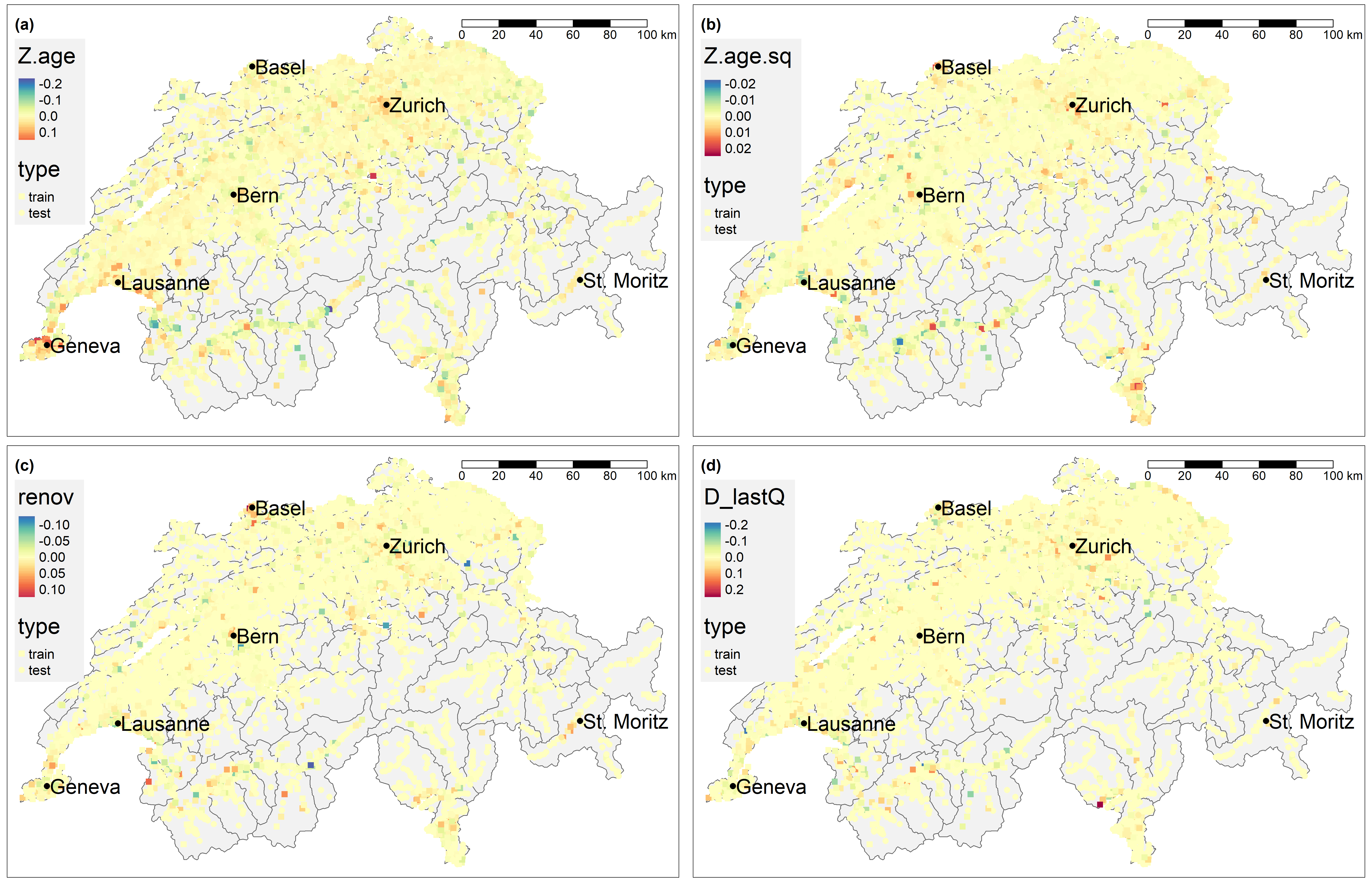
Finally, we show the other estimated SVC for fold , as we did in Figure 6 for the MLE.r method. These are the deviations from the corresponding mean , which added result in a single SVC for a covariate.
Age:
Of the four SVC yet not discussed in this paper, both the linear as well as quadratic effect of the age covariate have the most pronounced spatial structure, cf. Figure 14(a) and (b). One can see that the effect of age in agglomerations is very different from more rural areas. This is consistent with the assumption that – marginally – in rural areas one expects pure depreciation of an apartment with increasing age, while within city centers newly built and old (apartments with year of construction prior to 1920) are higher priced.
Renovation Rating and Last Quarter:
Both of theses covariates do not have very strong spatial structures, cf. Figure 14(c) and (d).