Cold gas and dust: Hunting spiral-like structures in early-type galaxies.

Abstract

Context. Observations of neutral hydrogen (H I) and molecular gas show that 50% of all nearby early-type galaxies contain some cold gas. Molecular gas is always found in small gas discs in the central region of the galaxy, while neutral hydrogen is often distributed in a low-column density disc or ring typically extending well beyond the stellar body. Dust is frequently found in early-type galaxies as well.

Aims. The goal of our study is to understand the link between dust and cold gas in nearby early-type galaxies as a function of H I content.

Methods. We analyse deep optical $g-r$ images obtained with the MegaCam camera at the Canada-France-Hawaii Telescope for a sample of 21 H I-rich and 41 H I-poor early-type galaxies.

Results. We find that all H I-rich galaxies contain dust seen as absorption. Moreover, in 57 per cent of these H I-rich galaxies, the dust is distributed in a large-scale spiral pattern. Although the dust detection rate is relatively high in the H I-poor galaxies ($\sim$59 per cent), most of these systems exhibit simpler dust morphologies without any evidence of spiral structures. We find that the H I-rich galaxies possess more complex dust morphology extending to almost two times larger radii than H I-poor objects. We measured the dust content of the galaxies from the optical colour excess and find that H I-rich galaxies contain six times more dust (in mass) than H I-poor ones. In order to maintain the dust structures in the galaxies, continuous gas accretion is needed, and the substantial H I gas reservoirs in the outer regions of early-type galaxies can satisfy this need for a long time. We find that there is a good correspondence between the observed masses of the gas and dust, and it is also clear that dust is present in regions further than $3\leavevmode\nobreak\ R_{\mathrm{eff}}$.

Conclusions. Our findings indicate an essential relation between the presence of cold gas and dust in early-type galaxies and offer a way to study the interstellar medium in more detail than what is possible with H I observations.

1 Introduction

Integral field spectroscopy shows that many, probably most, giant ellipticals and lenticulars (hereafter ETGs) contain an inner, fast rotating component ($<1R_{\mathrm{eff}}$) (e.g. Sarzi et al. 2006; Emsellem et al. 2007, 2011; Croom et al. 2012; Sánchez et al. 2012; Bundy et al. 2015). In those same inner regions, ionised gas is detected frequently (e.g. Rampazzo et al. 2005; Davis et al. 2011; Gomes et al. 2016; Gavazzi et al. 2018), and young stellar populations are not uncommon (e.g. Trager et al. 2000; Kaviraj et al. 2007; Kuntschner et al. 2010). Studies that are carried out with integral field units instruments, generally focus on the central regions of galaxies due to a small field of view (FOV) (e.g. Cappellari et al. 2011a; Laurikainen et al. 2011; Kormendy & Bender 2012; Krajnović et al. 2013; Weijmans et al. 2014). However, deep optical images show that we can study ETGs at considerable distance from the centre (Duc et al. 2014, 2015; Karabal et al. 2017). Moreover, these deep optical studies provide good quality data for not only the outer regions but also the inner regions of galaxies.

Similarly, observations of neutral hydrogen (H I) and molecular gas, such as CO, show that ETGs have gas discs (e.g. van Driel & van Woerden 1991; Young 2002; Morganti et al. 2006; Oosterloo et al. 2007, 2010; Crocker et al. 2011). Observations carried out as a part of the ATLAS^3D survey show that $\sim$50 per cent of all nearby ETGs contain some cold gas (CO and H I) (Young et al. 2011; Serra et al. 2012). The molecular gas is typically found in small gas discs in the central regions and is linked to small amounts of star formation (SF) (Alatalo et al. 2013; Davis et al. 2013). In contrast, H I has been found distributed in discs or rings that are much larger than the stellar body (Serra et al. 2012). If the column density of the gas is high enough, these H I discs host star formation with an efficiency (star formation per unit gas mass) similar to that in the outer parts of spirals (Yıldız et al. 2015, 2017).

Given their cold gas content, it is no surprise that many ETGs host some dust too. The presence of dust in these galaxies has long been known and discussed in the literature (e.g. Sadler & Gerhard 1985; Goudfrooij et al. 1994; Lauer et al. 1995; van Dokkum & Franx 1995; Ferrari et al. 1999; Tran et al. 2001). These studies indicate a relation between dust and ionised gas (e.g, see review by Ford et al. 1997). Previous studies have revealed dust structures in the very central regions of ETGs by using the Hubble Space Telescope (HST) (Simões Lopes et al. 2007; Martini et al. 2013). For example, Simões Lopes et al. (2007) have found complex dust structures in the very central regions of ETGs, and even some spiral-shape dust structures ($<$ 25 per cent).

Dust in ETGs is not only detected via absorption at optical wavelengths but also in emission in infrared (IR) bands, particularly in the far-IR (Knapp et al. 1989; Bregman et al. 1998; Pahre et al. 2004; Temi et al. 2007; Smith et al. 2012; di Serego Alighieri et al. 2013; Martini et al. 2013; Orellana et al. 2017). For example, by using Herschel observations, di Serego Alighieri et al. (2013) find that the dust mass of ETGs in the Virgo cluster ranges from $10^{4.9}$ to $10^{7}$ M_☉. Martini et al. (2013) also find a similar range of ETG dust masses, from $10^{5}$ to $10^{6.5}$ M_☉, based on Spitzer data.

One of the primary objectives of the above mentioned studies is to understand the origin of the dust and thus determine the following: whether it is internal (e.g. via mass loss from evolving stars), external (e.g. via galaxy minor mergers), or a combination of the two (as argued by Martini et al. 2013). Davis et al. (2015) claim that the dust in their sample of bulge-dominated galaxies with large dust lanes was accreted through minor mergers.

In this paper, we analyse ground-based deep optical images with lower angular resolution than the HST ones but with much higher radial coverage, which puts us in a position to study the origin of the dust in these galaxies. We aim to bring together the deep optical images and the H I, and if possible CO data to understand the relation between cold gas and dust across the entire stellar body. In particular, we try to understand whether the large H I discs play a role in the formation and evolution of the dust structures in the local ETGs. In order to do so, we investigated the distribution of dust in our sample galaxies by using deep colour maps (i.e. $g^{\prime}-r^{\prime}$). We classified the dust morphology and compared H I-rich to H I-poor ETGs. We modelled the dust-free colours in the galaxies and subtracted them from the colour maps to measure the colour excess. We verified whether the amount of colour excess is consistent with the known H I content. We also estimated the amount of dust in galaxies by using the total optical colour excess and compared our results to those obtained from far-IR observations.

We organise this paper in the following way. In Section 2, we describe the target and control sample selection. In Section 3, we describe the primary data (H I and optical) and the methodology used for our work, which includes modelling the dust-free colour, measuring the dust mass, the colour excess, and comparing it with the H I surface density in our sample galaxies, in particular. In Section 4, we present our results about the morphology of the dust structures by classifying them, their radial extent, and the dust mass. In Section 5, we discuss the relation between cold gas and dust by comparing the fraction of galaxies (i.e. detection rates) in the various dust morphological classes. We then discuss whether the age of the galaxies or misalignment between gas and stars play a role in the relationship between dust and H I. In Section 6, we present our conclusions.

Table 1: General properties of the H I-rich sample.

No	Name	$D$	$V_{\mathrm{hel}}$	$M_{K}$	log10($R_{\mathrm{eff}}$)	P.A.	$\varepsilon$	$E(B-V)$	log${}_{10}M$(H I  )	log${}_{10}M_{\star,r}$
		[Mpc]	[km/s]	[mag]	[arcsec]	[degrees]	[ ]	[mag]	[M☉]	[M☉]
	(1)	(2)	(3)	(4)	(5)	(6)	(7)	(8)	(9)	(10)
1	NGC 2594	35.1	2362	-22.36	0.82	306	0.122	0.050	8.91	10.47
2	NGC 2685	16.7	875	-22.78	1.41	37	0.402	0.051	9.33	10.31
3	NGC 2764	39.6	2706	-23.19	1.09	173	0.218	0.034	9.28	10.64
4	NGC 2859	27.0	1690	-24.13	1.43	269	0.272	0.017	8.46	10.97
5	NGC 3414	24.5	1470	-23.98	1.38	135	0.079	0.021	8.28	11.11
6	NGC 3522	25.5	1228	-21.67	1.01	241	0.504	0.020	8.47	10.31
7	NGC 3619	26.8	1560	-23.57	1.42	72	0.020	0.013	9.00	10.91
8	NGC 3626	19.5	1486	-23.30	1.41	179	0.454	0.017	8.94	10.54
9	NGC 3838	23.5	1308	-22.52	1.04	144	0.382	0.009	8.38	10.36
10	NGC 3941	11.9	930	-23.06	1.40	189	0.338	0.018	8.73	10.34
11	NGC 3945	23.2	1281	-24.31	1.45	159	0.435	0.023	8.85	11.02
12	NGC 3998	13.7	1048	-23.33	1.30	67	0.458	0.013	8.45	10.94
13	NGC 4036	24.6	1385	-24.40	1.46	272	0.507	0.019	8.41	11.16
14	NGC 4203	14.7	1087	-23.44	1.47	206	0.153	0.012	9.15	10.60
15	NGC 4278	15.6	620	-23.80	1.50	50	0.230	0.023	8.80	11.08
16	NGC 5173	38.4	2424	-22.88	1.01	261	0.214	0.024	9.33	10.42
17	NGC 5582	27.7	1430	-23.28	1.44	30	0.403	0.011	9.65	10.86
18	NGC 5631	27.0	1944	-23.70	1.32	34	0.198	0.017	8.89	10.89
19	NGC 6798	37.5	2360	-23.52	1.23	324	0.383	0.114	9.38	10.69
20	UGC 06176	40.1	2677	-22.66	1.03	210	0.598	0.015	9.02	10.44
21	UGC 09519	27.6	1631	-21.98	0.87	198	0.402	0.018	9.27	10.06

• Note.$-$ Column (1): The name is the principal designation from LEDA (Paturel et al. 2003). Column (2): distance in Mpc Cappellari et al. (2011a). Column (3): heliocentric velocity Cappellari et al. (2011a). Column (4): absolute magnitude derived from the apparent magnitude in K band Cappellari et al. (2011a). Column (5): projected half-light effective radius Cappellari et al. (2011a). Column (6): position angle of the galaxy calculated from the H I  image Serra et al. (2014). Column (7): ellipticity of the galaxy calculated from the H I  image Serra et al. (2014). Column (8): estimates of Galactic dust extinction Schlafly & Finkbeiner (2011). Column (9): total H I  mass calculated assuming galaxy distances given in column (2) Serra et al. (2012). Column (10): stellar mass calculated by using a mass-to-light ratio and a total luminosity in the r-band (Cappellari et al. 2013).

2 Sample

To study the relation between the dust distribution and the H I properties of ETGs, we selected an H I-rich sample and an H I-poor control sample. With a few exceptions, the two samples are the same as those studied in Yıldız et al. (2017) in which we studied ultraviolet (UV) properties in large H I discs (Serra et al. 2012). Compared to the H I-rich sample of Yıldız et al. (2017), we excluded galaxies in the Virgo cluster because we wish to limit the analysis to a field sample. Our final H I-rich sample includes 21 ETGs, which we list in Table 1. The H I-poor control galaxies are selected with properties as close as possible to the ones of the following H I-rich objects: i) stellar mass $M_{\star}$ (Cappellari et al. 2013) within +/- 0.8 dex, but typically within +/- 0.5 dex; ii) environment density $\Sigma_{3}$ (Cappellari et al. 2011b) within +/- 0.8 dex, but typically within +/- 0.5 dex iii) Virgo cluster non-membership (Cappellari et al. 2011a); iv) kinematical classification (fast or slow rotator; Emsellem et al. 2011); and v) distance (Cappellari et al. 2011a) within +/- 15 Mpc. With these requirements, we selected a control sample of 41 H I-poor ETGs, which are listed in Table 2. The distribution of effective radii $R_{\mathrm{eff}}$ for galaxies in this control sample is consistent with that for the HI-rich sample. Finally, ten (10/21) of our H I-rich galaxies are CO-rich, while only four out of the 41 H I-poor galaxies are CO-rich.

Table 2: Control sample galaxies for each H I-rich galaxy.

H I-rich	Control 1	Control 2	Control 3	Control 4
NGC 2594	NGC 5611	-	-	-
NGC 2685	NGC 2549	NGC 2852	NGC 5273	NGC 3098
NGC 2764	NGC 4078	NGC 2592	NGC 0770	-
NGC 2859	NGC 3230	NGC 3458	-	-
NGC 3414	NGC 5322	-	-	-
NGC 3522	NGC 3796	PGC 050395	-	-
NGC 3619	NGC 5308	NGC 3658	NGC 5342	-
NGC 3626	NGC 3377	NGC 5500	NGC 5473	-
NGC 3838	NGC 2950	NGC 4283	-	-
NGC 3941	NGC 3605	NGC 3301	NGC 3248	-
NGC 3945	NGC 3674	NGC 3648	-	-
NGC 3998	NGC 3610	-	-	-
NGC 4036	NGC 3613	NGC 6548	NGC 3665	UGC 08876
NGC 4203	NGC 3245	NGC 3757	-	-
NGC 4278	NGC 5485	-	-	-
NGC 5173	NGC 3400	-	-	-
NGC 5582	NGC 2577	NGC 2679	-	-
NGC 5631	NGC 0661	-	-	-
NGC 6798	NGC 6547	-	-	-
UGC 06176	UGC 04551	-	-	-
UGC 09519	NGC 7457	-	-	-

3 Data reduction and analysis

This work is based on a combination of radio and optical data. We use radio data from the Westerbork Synthesis Radio Telescope and make use of the H I images and $M$(H I) measurements (or upper limits) published by Serra et al. (2012) for all of the galaxies in our sample. That work also makes use of the data published previously by Morganti et al. (2006), Józsa et al. (2009), and Oosterloo et al. (2010) for some galaxies in our sample. In the remaining part of this section, we describe our analysis of the optical data.

3.1 MegaCam data reduction

We make use of deep optical images obtained in $g^{\prime}$ and $r^{\prime}$ bands by using the MegaCam camera on the Canada-France-Hawaii Telescope. The observations were obtained as part of the MATLAS/ATLAS^3D programme. Duc et al. (2015) describe all the details of these deep observations and of the data reduction, which makes use of the Elixir-LSB pipeline. Here, we remind the reader that the typical surface brightness sensitivity of these images is 28.5 mag arcsec^-2 in the $g^{\prime}$ and $r^{\prime}$ bands. For this work, we applied a few additional reduction steps, including background subtraction and point-spread-function (PSF) matching in the two bands.

In order to calculate the background of each image, we masked out all pixels above a one sigma level by using SExtractor (Bertin & Arnouts 1996). We then selected 20 regions, each $50\times 50$ pixels in size, and measured the median pixel value in each of them. We took the background level as the mean of these 20 median values and calculated its error as their standard deviation. We repeated this process for all $g^{\prime}$- and $r^{\prime}$-band images and subtracted the resulting background level.

Since we are interested in analysing the $g^{\prime}-r^{\prime}$ colour maps, we needed to first ensure that the images of the two bands have the same resolution. For this purpose, we measured the seeing (full width half maximum: FWHM) in the two bands by using five unsaturated stars located in relatively empty regions of the sky. We used IRAF - imexamine to measure the FWHM. We then corrected for the difference in seeing by smoothing the data of the band with the highest resolution to the lowest resolution band. After removing the background and matching the PSF in the two bands, we computed the calibrated colour maps.

3.2 Modelling dust-free colours and measuring the colour excess

In this work, we use the MegaCam $g^{\prime}-r^{\prime}$ deep colour maps to study the spatial distribution of the dust in H I-rich and H I-poor ETGs. The signal-to-noise ratio of the colour maps decreases with increasing radius. Therefore, we derived the radial profiles along annuli with a fixed shape (ellipticity and position angle) but which logarithmically increasing in width from inside out. The ellipticity and position angle of the annuli are fixed to the values published by Krajnović et al. (2011).

Before deriving the dust-free colour profiles, we masked the dusty regions in the images as much as possible. Here, we used a procedure that contains a combination of automatic and manual masking. We explain this procedure in detail in Appendix A. In summary, we i) took the median value of the clipped annulus as a first guess for the dust-free colour; ii) we repeated this for all the annuli and created a model; iii) we applied a median filter to remove sharp edges between annuli; iv) we required that the dust-free colour remains constant or becomes bluer when going outwards; and v) we finally forced the model to be a smooth function of radius since this kind of behaviour for ETGs is expected.

The best model representing the dust-free colour was subtracted from the original $g^{\prime}-r^{\prime}$ colour map to obtain a colour excess map. We limited our analysis to a maximum radius of 3 R_eff. The analysis of the colour profiles at a larger radius, which is beyond the scope of this paper, would require a more careful treatment of the effects of the PSF wings.

There are some uncertainties as to how the colour excess is calculated, which is based on the assumption that a dust-free colour can be obtained from the image and that the stellar populations do not change quickly with the radius. Also, we assume that no young stellar populations are present in the centre. This is not the case for some objects, such as NGC 2685. For this object, the measured colour excess is a lower limit. However, this problem is alleviated by the fact that young stars most likely occupy the same regions as the dust.

Having obtained the colour excess maps, we can calculate an average colour excess in a given annulus or a region. For this, we used the following equation:

$$\begin{aligned} \langle E(g^{\prime}-r^{\prime})\rangle\leavevmode\nobreak\ =\leavevmode\nobreak\ -2.5\times log_{10}(\frac{\Sigma(I_{r}\times R^{2}\times q\times 2.512^{-E(g^{\prime}-r^{\prime})})}{\Sigma(I_{r}\times R^{2}\times q)})\end{aligned},$$ (1)

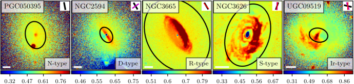
Figure 1: Example $g^{\prime}-r^{\prime}$ colour maps for our dust classification. The tick labels along the colour-bar indicate median$-4\sigma$, median$-2\sigma$, median, and median$+2\sigma$, respectively. The colour bars are limited between median$-5\sigma$ and median$+3\sigma$. The median and standard deviation values of the $g^{\prime}-r^{\prime}$ colour are calculated in the region of 0-1 R_eff, which is shown with the black ellipse. The white scale bar at the bottom corner indicates 1 kpc. On the top-right, we show an illustration of the position angles of the various galaxy components: in black the optical-disc from Krajnović et al. (2011); in purple the H I-disc from Serra et al. (2014); and in red the CO-disc from Alatalo et al. (2013). Similar $g^{\prime}-r^{\prime}$ colour maps of all of the galaxies studied here are shown in Appendix C.

where $I_{r}$ is the relative surface brightness (in intensity units) in the $r^{\prime}$-band, $R$ is the radius of the annulus, and $q$ is the flattening value of the annulus which is assumed to be constant throughout the galaxy. In Sec. B, we explain how we used these maps to estimate the amount of H I from the extinction caused by the dust.

3.3 Dust mass calculation and other parameters

There are several ways to estimate the dust mass of a galaxy. First, we estimated the dust mass by using the total extinction obtained from the colour excess maps (Sec. 3.2). For example, for this we followed the method used in the literature by Goudfrooij et al. (1994),Patil et al. (2007), and Finkelman et al. (2012) (see Sec. B for the equations and details for the optical method). As a second estimate, we adopted the dust mass values of Kokusho et al. (2019), which are based on the spectral energy distribution (SED) fits of Kokusho et al. (2017) for ATLAS^3D galaxies. Finally, the IR dust estimate based on the graphical method of Draine & Li (2007) could not be applied because the available mid- and far-IR data are of insufficient sensitivity.

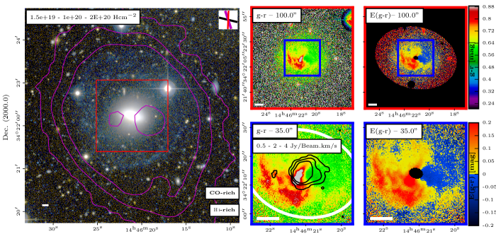
Figure 2: Left: True colour image of UGC 09519 with overlaid H I column density contours (magenta; see top-left box for the contour levels). The size of the true colour image is 300$\times$300 arcsec². Top-middle: $g^{\prime}-r^{\prime}$ image covering 100$\times$100 arcsec² area indicated in the left panel with a red box. Top-right: $E(g^{\prime}-r^{\prime})$ colour excess map (100$\times$100 arcsec²). Bottom-middle: $g^{\prime}-r^{\prime}$ image covering the 35$\times$35 arcsec² area indicated in the top-middle panel with a blue box. Since CO is generally detected in the inner regions, we show the CO intensity contours with black lines in this panel (see Alatalo et al. 2013). The white ellipse indicates the dust radius determined through visual inspection (see Table 3). Bottom-right: $E(g^{\prime}-r^{\prime})$ colour excess map (35$\times$35 arcsec²). The contour levels are indicated in the relevant panels. The white bar in the panels represents 1 kpc. On the top-right corner of the left panel, we also present the position angles as in Fig. 1. See Appendix C for the rest of the sample.

We make use of the data of Young et al. (2011) and Alatalo et al. (2013) who provide the total H₂ mass values and the distribution of CO emission (from the zero-moment maps), respectively. Young et al. (2011) used the Institut de Radioastronomie Millimetrique (IRAM) 30-metre single-dish radio telescope to look at the molecular gas content for all the ATLAS^3D galaxies. Alatalo et al. (2013) observed some of these CO-detected ETGs with the Combined Array for Research in Millimeter Astronomy (CARMA) interferometer. We retrieved the CO maps of Alatalo et al. (2013) to compare the dust and the CO distribution. We cannot compare H I and the other component of interstellar matter (ISM) since the resolution of the WSRT beam is much lower than those of the CARMA and the CHFT.

4 Results

4.1 Dust morphological classes

The first step of our analysis is a visual inspection of the MegaCam $g^{\prime}-r^{\prime}$ colour maps to establish which H I-rich and H I-poor galaxies harbour some dust. Almost all galaxies in our sample show redder colours in the inner regions. However, we label a galaxy as ‘dusty’: (i) if the reddened region is distinctly different from the underlying stellar body of the galaxy (either with a different morphology or a different position angle); and (ii) in case of a similar morphology and position angle, if the red colour is in excess of the model colour (see below). Otherwise, we label galaxies as no-dust objects (N). Our method for selecting dusty galaxies is somewhat conservative and, therefore, we may have missed some of them.

We classify the dust-detected ETGs as follows: dusty disc (D), irregular dust structure (Ir), dusty ring (R), and spiral shape (S). We present an example galaxy for each of these morphological types in Fig. 1. We show all the galaxies in Appendix D. Below, we elaborate on the characteristics of these classes.

When the position angle of these reddened regions is aligned with the stellar disc, it is hard to separate the dust from the old stellar populations. Either a large amount of dust or old and red stellar populations might cause the redder colours in these systems. Thus, for these cases, we calculated a theoretical $g^{\prime}-r^{\prime}$ colour with the following equation given by Bernardi et al. (2005):

$$g^{\prime}-r^{\prime}=\left\{\begin{array}[]{l}0.7\leavevmode\nobreak\ +\leavevmode\nobreak\ 0.25(T-9.5)\leavevmode\nobreak\ +\leavevmode\nobreak\ 0.375\leavevmode\nobreak\ Z\qquad\text{ if }T>9.5\\ 0.7\leavevmode\nobreak\ +\leavevmode\nobreak\ 0.50(T-9.5)\leavevmode\nobreak\ +\leavevmode\nobreak\ 0.375\leavevmode\nobreak\ Z\qquad\text{ if }T<9.5\end{array}\right.,$$ (2)

where T is the age in units of Gyr and $Z$ is the metallicity. This equation estimates a $g^{\prime}-r^{\prime}$ colour for stellar populations older than 1 Gyr based on the single-burst models of Bruzual & Charlot (2003). We used the stellar ages and metallicity values from McDermid et al. (2015) and we classify a galaxy as a D object, that is, a galaxy with a dusty disc, if the observed g’-r’ colour is redder than the theoretical one given the high surface brightness in the inner regions. We can trust a small difference between the observed and theoretical colours (e.g. 0.01 mag). It is important to note that we only used this test if a galaxy has a red disc-type region that is well aligned with the stellar component (six galaxies in our sample).

Many of the galaxies in our sample show a ring-like structure in the very central regions ($\sim<0.5$ kpc). However, since a number of galaxies are saturated in the centre, we did not take these very inner regions into account. Therefore, only if a galaxy exhibits a relatively sizeable ($>0.5$ kpc) dusty ring do we label it as an R object (see Fig. 1).

Several galaxies in our sample exhibit dust that is distributed in a spiral pattern. In these cases, we label them as S galaxies. These spiral-shaped arms could be confined to a relatively inner region, but in several cases, they reach a large radius (see Fig. 1). Some of the galaxies show very complex dust structures, and we label them as irregular (Ir) dusty galaxies.

We list our classification together with those of Krajnović et al. (2011) for all the sample galaxies in Table 3. We quantify the colour excess and the amount of dust in the next sections. We detected dust in a total of 44 galaxies, which is 71 per cent of our sample of 62 ETGs. Out of these, 12, 14, 6, and 12 are S-, IR-, R-, and D-type, respectively.

Table 3: Dust morphology, extension, and mass for the H I-rich and H I-poor galaxies.

Gal	Dist.	log${}_{10}R_{\mathrm{eff}}$	q	HI-Typec	Dust morphology			Dust Radius
	[Mpc]	[arcsec]	-	-	SL07-T01	K11	This work	[arcsec]	[$R_{\mathrm{eff}}$]	[Kpc]
(1)	(2)	(3)	(4)	(5)	(6)	(7)	(8)	(9)	(10)	(11)
NGC 0661	30.6	1.12	0.69	Poor	-	N	N	0	0.0	0.0
NGC 0770	36.7	0.94	0.71	Poor	-	N	D	5	0.6	0.9
NGC 2549	12.3	1.28	0.31	Poor	-N	N	N	0	0.0	0.0
NGC 2577	30.8	1.15	0.59	Poor	-	N	Ir	14	1.0	2.1
NGC 2592	25	1.09	0.79	Poor	-D	N	N	0	0.0	0.0
NGC 2594	35.1	0.82	0.68	Rich	-	N	D	10	1.5	1.7
NGC 2679	31.1	1.35	0.93	Poor	-	N	N	0	0.0	0.0
NGC 2685	16.7	1.41	0.6	Richc	-	F	S	100	3.9	8.1
NGC 2764	39.6	1.09	0.51	Richc	-	FB	S	35	2.8	6.7
NGC 2852	28.5	0.85	0.86	Poor	-	N	R	12	1.7	1.7
NGC 2859	27	1.43	0.85	Rich	-	N	S	22	0.8	2.9
NGC 2950	14.5	1.19	0.59	Poor	N-N	N	N	0	0.0	0.0
NGC 3098	23	1.12	0.23	Poor	-	N	D+	50	3.8	5.6
NGC 3230	40.8	1.26	0.39	Poor	-	N	N	0	0.0	0.0
NGC 3245	20.3	1.40	0.54	Poorc	-	N	Ir	15	0.6	1.5
NGC 3248	24.6	1.20	0.6	Poor	-	N	D	5	0.3	0.6
NGC 3301	22.8	1.30	0.31	Poor	-	N	Ir	11	0.6	1.2
NGC 3377	10.9	1.55	0.67	Poor	l,0.26-F1	N	Ir	19	0.5	1.0
NGC 3400	24.7	1.23	0.56	Poor	-	N	N	0	0.0	0.0
NGC 3414	24.5	1.38	0.78	Rich	S,0.15-F1	N	S	30	1.3	3.6
NGC 3458	30.9	1.06	0.71	Poor	-	N	N	0	0.0	0.0
NGC 3522	25.5	1.01	0.52	Rich	-	N	Ir	8	0.8	1.0
NGC 3605	20.1	1.23	0.6	Poor	-	N	R	7	0.4	0.7
NGC 3610	20.8	1.20	0.81	Poor	N	N	N	10	0.6	1.0
NGC 3613	28.3	1.42	0.54	Poor	-N	N	N	0	0.0	0.0
NGC 3619	26.8	1.42	0.91	Richc	-	FBR	S	40	1.5	5.2
NGC 3626	19.5	1.41	0.67	Richc	-	D	S	30	1.2	2.8
NGC 3648	31.9	1.12	0.56	Poor	-	N	N	0	0.0	0.0
NGC 3658	32.7	1.28	0.84	Poor	-	N	N	0	0.0	0.0
NGC 3665	33.1	1.49	0.78	Poorc	-	D	R	18	0.6	2.9
NGC 3674	33.4	1.05	0.36	Poor	-	N	N	0	0.0	0.0
NGC 3757	22.6	0.95	0.85	Poor	-	N	N	0	0.0	0.0
NGC 3796	22.7	1.06	0.6	Poor	-	N	Ir	7	0.6	0.8
NGC 3838	23.5	1.04	0.44	Rich	-	N	Ir	9	0.8	1.0
NGC 3941	11.9	1.40	0.75	Rich	-	N	Ir	26	1.0	1.5
NGC 3945	23.2	1.45	0.65	Rich	i,x,	FBR	S	60	2.1	6.8
NGC 3998	13.7	1.30	0.78	Rich	il,0.43	N	Ir	35	1.8	2.3
NGC 4036	24.6	1.46	0.4	Richc	il,x	F	S	30	1.0	3.6
NGC 4078	38.1	0.92	0.44	Poor	-	N	D	8	1.0	1.5
NGC 4203	14.7	1.47	0.89	Richc	sl,0.23	N	S	50	1.7	3.6
NGC 4278	15.6	1.50	0.91	Rich	i,x	N	Ir	30	0.9	2.3
NGC 4283	15.3	1.09	0.96	Poorc	-	N	D	8	0.7	0.6
NGC 5173	38.4	1.01	0.87	Richc	-F3	B	Ir	23	2.2	4.3
NGC 5273	16.1	1.57	0.84	Poorc	sl,0.14	N	Ir	18	0.5	1.4
NGC 5308	31.5	1.25	0.2	Poor	N-N	N	D+	50	2.8	7.6
NGC 5322	30.3	1.60	0.64	Poor	-	N	N	0	0.0	0.0
NGC 5342	35.5	0.97	0.46	Poor	-	N	D	18	1.9	3.1
NGC 5473	33.2	1.32	0.79	Poor	-	N	N	0	0.0	0.0
NGC 5485	25.2	1.45	0.74	Poor	-	D	R	25	0.9	3.1
NGC 5500	31.7	1.18	0.8	Poor	-	N	N	0	0.0	0.0
NGC 5582	27.7	1.44	0.65	Rich	-	N	D	8	0.3	1.1
NGC 5611	24.5	1.00	0.45	Poor	-	N	D	6	0.6	0.7
NGC 5631	27	1.32	0.93	Rich	-	D	S	35	1.7	4.6
NGC 6547	40.8	1.06	0.33	Poor	-	N	D+	25	2.2	4.9
NGC 6548	22.4	1.35	0.89	Poor	-	N	R	12	0.5	1.3
NGC 6798	37.5	1.23	0.53	Richc	-	N	S	30	1.8	5.5
NGC 7457	12.9	1.56	0.53	Poor	N	N	D	15	0.4	0.9

Table 3: Continued

Gal	Dist.	log${}_{10}R_{\mathrm{eff}}$	q	HI-Typec	Dust morphology			Dust Radius
	[Mpc]	[arcsec]	-	-	SL07-T01	K11	This work	[arcsec]	[$R_{\mathrm{eff}}$]	[Kpc]
(1)	(2)	(3)	(4)	(5)	(6)	(7)	(8)	(9)	(10)	(11)
PGC 050395	37.2	1.04	0.73	Poor	-	N	N	0	0.0	0.0
UGC 04551	28	1.03	0.39	Poor	-N	N	Ir	10	0.9	1.4
UGC 06176	40.1	1.03	0.51	Richc	-	F	S	31	2.9	6.0
UGC 08876	33.9	0.93	0.37	Poor	-	N	R	12	1.4	2.0
UGC 09519	27.6	0.87	0.75	Richc	-	F	Ir	20	2.7	2.7

• Note.$-$ Column (1): The name is the principal designation from LEDA (Paturel et al. 2003). Column (2): distance in Mpc Cappellari et al. (2011a). Column (3): projected half-light effective radius Cappellari et al. (2011a). Column (4): the ratio of the minor axis to the major axis obtained from the ellipticity value Krajnović et al. (2011). Column (5): H I  content of the galaxy (Serra et al. 2012). The ^c sign indicates CO detection (Young et al. 2011). Column ($6-7$): Labels used to define the dust morphology in the previous studies: Simões Lopes et al. (2007) and Tran et al. (2001) (6); Krajnović et al. (2011) (7). If the size of the dust structure is given in the previous studies, we give this value next to the label. Column (8): labels used to define the dust morphologies in this study. Column ($9-11$): Dust radius measured in this study in the units of arcsec, effective radius, and Kpc, respectively. Column ($12$): Estimated dust masses from the total optical extinction ($A(g^{\prime})$). Column ($13$): Dust masses derived from SED fits by using far-IR data (Kokusho et al. 2019).
  Comments.$-$ Labels of the dust morphological classes, D: dusty disc; Ir: irregular dust; R: dusty ring; S: spiral-shaped structure; N: no-dust structure; D⁺: almost edge-on dusty disc. Labels used in the previous studies are different than our classes: F1: filamentary low; F3: filamentary high; l: dust lane or filament.

4.2 Extended dust structures and relation with the cold gas properties

A significant result of our study is the distribution of the dust features in ETGs. For the first time, our results show the detailed distribution of the dust in ETGs up to a large radius. In Table 3, we list the dust radii estimated visually based on our MegaCam images and, for comparison, those available in the literature. As an example, Fig. 2 shows the $g^{\prime}-r^{\prime}$ and $E(g^{\prime}-r^{\prime})$ images of UGC 9519 together with an ellipse indicating the dust radius. The white ellipse in Fig. 2 has a semi-major axis that is equal to the dust radius, as well as the position angle and ellipticity from Krajnović et al. (2011).

The average dust radius across the sample is $\sim$ 2.9 $\pm$ 0.3 kpc (1.3 $\pm$ 0.1 R_eff). There are three nearly edge-on galaxies in our sample (inclination $>$ 80 deg, labelled as D⁺ in Table 3), and since the sensitivity to dust absorption increases with increasing inclination, it is easier to detect dust in these galaxies. If we do not take into account these galaxies, the average dust radius becomes $\sim$ 2.6 $\pm$ 0.3 kpc, which is not very different.

Here we discuss the dust radius as a function of cold gas content. As can be seen in Table 3, in all the S-type galaxies, which are also H I-rich, the dust extends further than 3.5 kpc. We find the average dust radius for the H I-rich and H I-poor ETGs to be $\sim$ 3.7 $\pm$ 0.4 kpc and $\sim$ 2.1 $\pm$ 0.3 kpc, respectively. However, if we do not take into account the nearly edge-on systems, the average value for H I-poor ETGs becomes $\sim$ 1.4 $\pm$ 0.2 kpc, while the average value does not change for the H I-rich ETGs. Therefore, we can conclude that H I-rich ETGs contain about a two times larger dust structure than H I-poor ETGs. If we define gas-rich galaxies as those detected in either H I  or CO, then we find that the dust structures extend to $\sim$ 3.3 $\pm$ 0.4 and $\sim$ 1.6 $\pm$ 0.3 kpc in gas-rich and gas-poor galaxies, respectively. The average dust radius for the CO-rich (H I-poor) galaxies is the same as the gas-poor galaxies. The S-type dust structures (present in only gas-rich ETGs) can reach out to $\sim$ 5 $\pm$ 0.5 kpc from the galaxy centre. Irregular dust structures (S+Ir) in gas-rich systems extend up to $\sim$ 4 $\pm$ 0.3 kpc. Therefore, we conclude that if there is cold gas in a galaxy (with H I), the dust structures extend to two times larger radii (on average) than in a gas-poor galaxy.

The principal goal of this work is to understand the relation between dust and cold gas, mainly H I, in ETGs. In this respect, we find an unambiguous result: all H I-rich ETGs in our sample host dust (mostly undetected in Krajnović et al. (2011)), while the dust detection rate of H I-poor galaxies is just 56 per cent. The presence of H I, anywhere in the galaxy, dramatically increases the dust detection rate of ETGs in the inner 3 R_eff. It is important to note that we can identify dust structures extending out to more than 3 R_eff, but we do not study these dust structures in this paper. We show the number of galaxies in each class based on their cold gas content in Fig. 3. As can be seen from the figure, all the S-type ETGs contain large H I-discs.

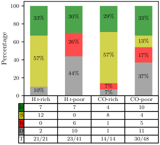
Figure 3: Number of galaxies containing dust according to their dust-type and cold gas content. The colour code is based on dust morphology defined in this paper. The percentage of the groups are written on the related bars, and the quantities are given in the lower table. The bottom row presents the total number of dusty galaxies for each gas content class.

We conclude that the presence of H I out to large radii always implies the presence of dust in the stellar body, whereas the opposite is not true. This is also the case for the CO-rich ETGs based on the results of Young et al. (2011), but it is important to note that these are not all the same objects as our H I-rich ones. In general, more nearby ETGs have been detected in H I than in CO (especially outside the Virgo cluster). ETGs that host a small H I disc, which we do not study in this work, also fit in this picture: nearly all of them host CO and dust (Serra et al. 2012).

Another notable result of this study is that we only detected spiral-shaped dust distributions in H I-rich galaxies (8/12 are also CO-rich; see Fig. 3). Moreover, 90 per cent of the dusty H I-rich galaxies (19 out of 21) shows complex dust structures that are either irregular or spiral in shape. In other words, the difference between gas-rich and gas-poor galaxies is even more dramatic if we consider the spatial distribution of the dust. We present a histogram in Fig. 4 showing the number of galaxies with and without H I for the large and small dust structures. As can be seen in the histogram, large dust structures tend to be in H I-rich galaxies while the small size dust structures reside in the H I-poor ETGs.

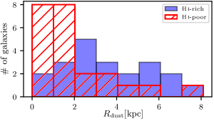
Figure 4: Histogram showing the number of galaxies as a function of dust radius. Small (i.e. $R_{\mathrm{dust}}\leq$ 1 kpc) and large (i.e. $R_{\mathrm{dust}}>$ 1 kpc) dust structures tend to be in H I-rich (blue bars) and H I-poor (red hatched bars) ETGs, respectively.

4.3 Colour excess and H I radial profiles

We propagated the errors on the colour profiles and calculated the average colour excess in each annulus by using Eq. 1. We also estimated the H I surface density of each annulus based on the colour excess as explained in Appendix B, and compared it with observed H I and CO profiles. This allowed us to test whether the radial distribution of the colour excess and that of the cold gas are related. We provide all the radial profiles of the sample galaxies in Appendix D.

In addition to the estimation of the H I surface density in each annulus, we also estimated the total H I mass in the region between 0-3 R_eff (see Appendix B). We plotted the estimated and observed values in this aperture in Fig. 5.

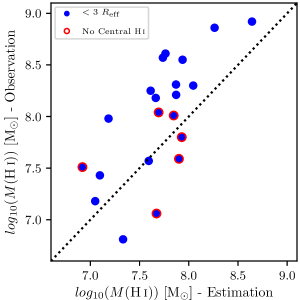
Figure 5: Observed H I  mass vs. the H I  mass estimated based on the colour excess (see text). The observed H I  mass was calculated based on the H I  images in Serra et al. (2012) within the same region where we detected a colour excess. The dotted line shows the one-to-one relation. Red outer circles indicate galaxies with no central H I ($<$ 1 R_eff).

As can be seen from the figure, the galaxies follow the one-to-one relation with a scatter. We note that six H I-rich galaxies (NGC 2859, NGC 3941, NGC 3945, NGC 4036, NGC 4278, and NGC 5582) in our sample have enormous H I ring or disc structures, while they have no H I in their very central regions (red circles in Fig. 5). While these galaxies show very red colours in the inner regions due to dust, they show blue colours in the outer regions where the highest H I column density rings are located (Yıldız et al. 2017). We would like to point out that these galaxies are also CO-poor with the exception of NGC 4278. Therefore, we conclude that the presence of a large H I disc or ring in an ETG indicates a dust structure in the centre, even if there is no H I in central regions. It would be interesting to continue to study these objects in future studies. Considering that our H I mass estimate in Fig. 5 is based on the colour excess-H I relation of the Milky Way (Appendix A), Fig. 5 suggests that H I-rich ETGs follow a different relation than our Galaxy.

5 Discussion

5.1 Dust detection rate and extension

The wide-field, deep optical images analysed here allow for a more complete characterisation of the distribution of dust in nearby, non-cluster ETGs than in previous works. As a result, we find that more than half of these galaxies (both gas-rich and -poor) contain dust structures (71 $\pm$ 6 per cent).

Our dust detection rate is much higher than that reported by Krajnović et al. (2011) for the full ATLAS^3D sample based on SDSS images, which is 19 per cent (this rate also holds for the 62 galaxies that are in common with our study alone). Therefore, the dust detection rate increases by a factor of approximately four when going from an SDSS-like depth and resolution to that of our MegaCam images. Images obtained with the HST, therefore, are more sensitive than the SDSS ones in the centre, and they give an ETG dust detection rate of $\sim$ 50 per cent, which is closer to those reported here. For example, Lauer et al. (2005) detected dust in 47 per cent of all galaxies in their sample of 77 ETGs.

In previous work based on the HST data, our D objects are typically not labelled as dusty, but this is primarily due to definition criteria (see Sec. 4.1). For example, Lauer et al. (2005) had stricter requirements for the position-angle misalignment. They did not classify a galaxy as dusty if the dust and stars are aligned (same position-angle). If we ignore the 12 D objects in our sample, the dust detection rate becomes entirely consistent with that of previous HST studies (32/62 = 52 $\pm$ 6 per cent). Concerning the remaining dusty galaxies, 10/12 S, 6/14 Ir, and 2/6 R were already known to host dust, although the dust distribution could not be studied to the same large radius as in this work.

Using HST images of 68 galaxies, Simões Lopes et al. (2007) found that 63 per cent of their sample contains dust structures and all the observed dust is in the central kiloparsec region. However, we find that most of the ETGs ($\sim$ 77 per cent) have extended dust structures more than 1 kiloparsec (see Fig. 4). Therefore, our study complements the previous investigations carried out using the HST data. For example, while the circumnuclear dust structure in NGC 4203 as seen by the HST extends up to just 0.23 kpc (Simões Lopes et al. 2007), our study shows that the spiral dust structures extend up to 2 kpc (see also Yıldız et al. 2015). One should consider that while we use deep optical $g^{\prime}-r^{\prime}$ colours to define the dust structures in ETGs, these authors use unsharp-masked, single-band HST images.

Finally, Carollo et al. (1997) showed that NGC 5322 has a clear dust structure; however, we do not label this galaxy as dusty. Lauer et al. (2005) claimed that virtually all the dust is located in the central 4 arcsec² region. In the deep MegaCam colour map, this galaxy has a saturated central part, and, therefore, we cannot identify the dust structure.

Dust detection is easier when the inclination of a galaxy is higher. Therefore, we checked whether the dust radius is related to the ellipticity (a proxy for inclination), and we present our result in Fig. 6. We conclude that gas-rich ETGs contain more extended dust than gas-poor ETGs regardless of the inclination. We do find a significant correlation between the dust radius and axis ratio for gas poor galaxies, which could be expected for galaxies with optically thin dust structures.

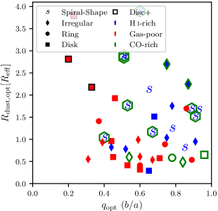
Figure 6: Dust radius as a function of ellipticity. The colours of the markers indicate gas content of the galaxies. The green hexagons indicate galaxies detected in CO. The ’Disc+’ legend (black marker edge colour) indicates galaxies with high inclination i.e. $\gtrsim$ 80 degrees.

Our detection rates based on dust absorption are similar to those reported in studies using infrared emission data. For example, Smith et al. (2012) report that the detection rate is 24 per cent and 62 per cent for elliptical and lenticular galaxies, respectively. The overall detection rate for their ETGs is $\sim$ 48 per cent. In a similar study, but only for Virgo ETGs, di Serego Alighieri et al. (2013) detect dust in 41 per cent of the lenticulars, and 17 per cent of the ellipticals (32 per cent for all ETGs).

Although the overall detection rate of di Serego Alighieri et al. (2013) is close to our results, they find dust in half of their H I detected galaxies (8/16). Yet, we find that all large H I disc galaxies, which are all outside of Virgo, contain dust. Their lower detection rate might be partly due to the fact that they searched for dust at the position of the optical galaxy centre, while in reality dust can be offset from that.

Serra et al. (2012) report 43 $\pm$ 9 per cent CO and dust detection rate in all H I-rich ETGs by using the study of Krajnović et al. (2011). If we revisit their study, a similar rate holds for our gas-rich ETGs (44 $\pm$ 10). However, by using deep-optical imaging, we find that all the gas-rich galaxies contain dust structures.

5.2 Dust mass

As discussed in the previous section, we find a different dust morphology in the H I-rich and H I-poor ETGs thanks to deep optical imaging. Yet, the question is begged as to whether we can properly measure the mass of dust in ETGs. In order to answer this question, we used the total extinction and calculated the dust mass for our sample galaxies, and then we compared our results with those derived from the SED fits including far-IR data (Kokusho et al. 2019). We tabulated the resulting dust masses in Table 5.

Not surprisingly, by using optical images, we underestimated the dust mass for most of the sample ETGs, which is similar to what was found in previous studies (e.g. Patil et al. 2007; Finkelman et al. 2012; Kaviraj et al. 2012; Viaene et al. 2015). Fig. 7 shows the comparison between our results and those obtained from far-IR emission. However, our result that the dust mass obtained from the total extinction value is six times higher in gas-rich than in gas-poor galaxies is consistent with previous studies (see comparison in Table 4).We also find that the correlation coefficients and p-values of the relation shown in Fig. 7 are $0.41-0.05$ and $0.18-0.51$ for the gas-rich and gas-poor galaxies, respectively. Although the significance of the correlation is low, it does increase for gas-rich ETGs.

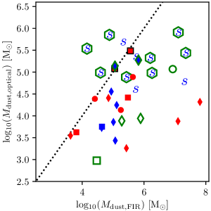
Figure 7: Dust masses estimated from optical absorption in this study vs. infrared emission (Kokusho et al. 2019). The black dotted line shows the one-to-one relation. The symbols are the same as in Fig. 6.

Table 4: Comparison of the average dust masses for gas-rich (GR) and gas-poor (GP) galaxies.

$M_{\mathrm{dust,GR}}$	$M_{\mathrm{dust,GP}}$	GR/GP	$M_{\star}$ range	Ref.
$\mathrm{M}_{\sun}$	$\mathrm{M}_{\sun}$	-	$\mathrm{M}_{\sun}$
5.2	4.4	6.3	$\sim$10.0 - 11.5	1
6.5	6.4 (5.8)	5.0	$\sim$10.0 - 11.5	2
6.5	5.9	4.0	$\sim$9.0 - 11.5	3
6.5	5.9	4.0	$\sim$8.5 - 11.0	4

• (1) This work. (2) Kokusho et al. (2019) (3) di Serego Alighieri et al. (2013) (4) Smith et al. (2012).
  

In Table 4, the reason for the small difference between gas-rich and gas-poor galaxies in Kokusho et al. (2019) is that two galaxies are contaminated or miss-classified: NGC 2577 and NGC 3301. As can be seen in Fig. 7, these galaxies have the highest estimated dust mass. However, the data of NGC 2577 comes from IRAS observations, and there is a nearby large spiral galaxy $\sim$ 6 arcmin north-west. Moreover, these two galaxies are located in a similar direction with the IRAS scanning track. Therefore, the high dust mass of this galaxy is likely due to the contamination from the nearby source. For NGC 3301, single-dish observations detected H I in this galaxy (Springob et al. 2005). However, we consider it as gas-poor since it was not detected in Serra et al. (2012). If we remove these two galaxies, the difference between the logarithmic dust mass of gas-rich and poor galaxies becomes 0.7 dex, which is similar to our result obtained based on the optical data.

It is clear that the ratio of dust mass between the gas-rich and gas-poor ETGs ($\frac{M_{d,GR}}{M_{d,GP}}=\sim 5$) is similar regardless of whether we use optical, 140 $\mu$m or 500 $\mu$m data. Moreover, it is the same for the field and cluster ETGs. These results are most likely due to a different origin of the gas and dust in these galaxies. Although far-IR data provides a better way to measure dust mass, the spatial resolution is very low at the long wavelengths. On the other hand, as we discussed in Sec. 5.1, deep optical images provide excellent data to study the spatial distribution of the dust in ETGs.

5.3 Origin of the dust

The origin of the dust in ETGs has been long discussed in the literature. These discussions follow two main lines: internal dust production and external dust accretion. There are also studies, such as Martini et al. (2013), which favour a mixed origin instead of a single one. There are uncertainties regarding the way in which the presence of cold gas in ETGs is linked to the origin of the dust.

If the stellar evolution is responsible for the dust produced in galaxies, we should see a correlation between the dust mass and the stellar mass of galaxies, especially if they are similar in terms of morphology, star formation history, and environment. Kokusho et al. (2019) find no such correlation and conclude that stellar mass loss is not a significant source of dust in ETGs.

The spiral shapes, irregular and clumpy dust distributions, and physical extent of the dust in H I-rich ETGs indicate that the dust was most likely accreted through a gas-rich minor merger. Our conclusion is supported by the fact that extended H I in several of these galaxies often comes from the external sources, as implied by the lack of a correlation between H I mass and stellar mass in ETGs (Serra et al. 2012) and by the frequent kinematical misalignment between H I and stars (Serra et al. 2014). Our results are also consistent with previous studies, such as Davis et al. (2015), who find that the origin of the cold gas is most likely due to the minor mergers in their sample ETGs (see also Geréb et al. 2016). Kaviraj et al. (2012) also stress that dust contribution from stellar mass loss is not enough to create the observed dust alone. Moreover, it is possible that dust is coupled with the H I in the very outer regions, and, therefore, could survive the interactions with the hot gas when accreting towards the centre (see also Finkelman et al. 2012).

In H I-poor ETGs, dust is mostly detected in the central regions. This is different from H I-rich galaxies and suggests that the dust origin is likely different. It is possible that dust in H I-poor ETGs mostly has an internal origin. Indeed, another scenario proposed by Temi et al. (2007) might be valid for gas-poor ETGs: cold dust is buoyantly transported from the core of the galaxies, where old stellar populations are located and dust is produced via stellar evolution. They claimed that active galactic nucleus energy outbursts might drive the buoyant outflow and cause the widespread dust distribution observed in optical colour maps.

As mentioned in the Introduction, Martini et al. (2013) discuss a hybrid model that includes both external accretion and internal dust production, which is further supported by recent studies (e.g. Bassett et al. 2017). For this hybrid model, they require low metallicity gas, and dusty ETGs should experience more mergers than dust-free galaxies. In this model, the external accretion of cold gas can be responsible for the dust distributions observed in ETGs. Our H I-rich ETGs have a vast gas reservoir, and the depletion time of the H I gas varies between 10 Gyr and 100 Gyr when moving from the inner regions to the outer regions (see Yıldız et al. 2017). The lifetime of H I and dust is most likely similar in the field, and, therefore, there is enough gas to accrete and prevent the dust structures from being depleted.

As a final note, we remind the reader that our sample of nearby ETGs includes only galaxies outside massive clusters. Our results may not hold for galaxies in clusters, where the environment could significantly affect the relation between gas at a large radius and dust in the stellar body. In the case of field galaxies, though, we conclude that the primary factor for the presence of dust in gas-rich ETGs is the external sources.

6 Conclusions and future prospects

We used deep optical images to study the distribution of dust in nearby ETGs. Thanks to the excellent resolution of the MegaCam images, we can classify the dust morphology in these ETGs. We compared H I-rich and H I-poor ETGs to understand whether the presence of dust and its spatial distribution are related to the presence of a large, extended reservoir of H I in these galaxies.

1- We find that all of the H I-rich galaxies show dusty structures, while 56 per cent of the H I-poor galaxies show dust.

2- In 76 per cent of the H I-rich galaxies, the dust distribution has a spiral-like morphology.

3- The spatially extended dust structures tend to be in H I-rich galaxies, while the small size dust structures are generally found in the H I-poor ETGs.

4- All of the galaxies with H I in the outskirts, but not in the centre, host dust in the relatively inner regions. Therefore, the presence of dust is linked to the presence of H I even when the H I is found at a much larger radius. These dusty inner regions may also indicate that cold gas used to be present in the centre of these galaxies.

5- Gas-rich ETGs contain less regular dust systems, which extend to a larger radius than gas-poor objects.

Given the extended and complex morphology of dust in H I-rich ETGs, and the fact that the H I is mostly accreted externally in these galaxies, we conclude that external accretion appears to be the dominant source of dust in these objects. As seen above, it is clear that there is a relation between the dust and cold gas (H I and CO) presence in ETGs.

7 Acknowledgements

MKY acknowledges the financial support from the Scientific and Technological Research Council of Turkey (TUBITAK) under the postdoc fellowship programme 1059B191701226. We also thank Tom Jarrett and Martin Bureau for valuable discussions on the infrared emission and dust mass calculations.

Appendix A Model calculation

In this appendix we give the details of the procedure used to calculate the dust-free colour from the $g^{\prime}-r^{\prime}$ images. In order to calculate the dust-free colours, we first needed to mask out all regions with dust, and to do this we started by automatically finding a masking threshold. To do so, we did the following: (1) We took a 100$\times$100 pixel² central area from the $g^{\prime}-r^{\prime}$ images and calculated its mean and standard deviation ($\sigma$) value. (2) We masked out all pixels above $mean+4\sigma$ and below $mean-4\sigma$. (3) We calculated the median and standard deviation from the remaining pixels. (4) We masked all pixels above and below $median\pm 3\sigma$ in the original image.

Having inspected the images, additional regions are manually masked if it is necessary. This masking procedure removes most of the dusty regions in the inner regions and also the noisy pixels in the outer regions. Having applied the masking procedure, we derived the profiles (as explained in Sec. 3.2). There is a possibility that a small part of the galaxy might contain a star-forming region. In this case, the dust-free colour is bluer than it should be, and the colour excess is overestimated. Therefore, we did not directly average the pixels in an annulus. Instead, we used four quadrants and a second masking process as follows:

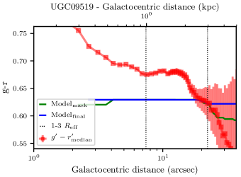
Figure 8: Radial profiles for the $g^{\prime}-r^{\prime}$ images and the two models obtained in our dust-free colour calculation process. The red profile shows the median colour value of the original annuli. The green line shows the model, which follows the requirement that the colour cannot get redder with increasing radius (see text). The blue profile shows the final model, which is flat before 0.5 $R_{\mathrm{eff}}$, and after 3 $R_{\mathrm{eff}}$. The dotted vertical lines indicate 1 $R_{\mathrm{eff}}$ and 3 $R_{\mathrm{eff}}$, respectively.

(a) We divided each annulus into four quadrants, and masked the pixels above median$+1.5\sigma$ and below median$-3\sigma$ in each quadrant. Here, we estimated the standard deviation by using the median absolute deviation. Using this asymmetric masking removes remaining red pixels in the annulus and keeps the blue pixels. (b) We calculated the median value from the remaining pixels in each quadrant for each annulus. This results in four median values representing the dust-free colours in the quadrants. (c) To get a better dust-free colour value, we used the second minimum of these four median values mentioned above as the dust-free colour. (d) Having derived the profiles, we applied a seven-pixel size median filter to remove sharp changes between the annuli.

The two-step process given above creates the first model for the dust-free colour. We manipulated this first model as follows: (i) We set the colour within $R_{\mathrm{eff}}$/2 to the value at $R_{\mathrm{eff}}$/2. If an effective radius is larger than 15 arcsec, we used the colour at 7.5^′′. (ii) Since early-type galaxies without a significant cold ISM are known to have smooth colour profiles, which become slowly bluer with an increasing radius beyond $R_{\mathrm{eff}}$/2 (e.g. Franx et al. 1989; Peletier et al. 1990, 1999, 2012), we did not allow our model to become redder towards a larger radius. Therefore, the model can either become bluer or stay constant when going outwards. (iii) We smoothed the model to remove the sharp edges. (iv) We assumed that the model colour does not change after 3 $R_{\mathrm{eff}}$ and we obtained our final model to represent a dust-free colour. (v) We calculated the errors on the colour (based on the errors in $g^{\prime}$ and $r^{\prime}$ bands, see Sec. 3.1 for details), and we truncated the colour radial profile at the first annulus where the error is higher than 0.2 mag, or at 3 $R_{\mathrm{eff}}$ at most. We show the original and masked $g^{\prime}-r^{\prime}$ median profiles together with the three model radial profiles in Fig. 8. In Fig. 8, the models are always below the $g^{\prime}-r^{\prime}$ colour profile because of the masking procedure explained above.

Appendix B H I and dust mass estimation

Our sample selection is based on H I detectability, and since we measured the colour excess in our sample galaxies, we can apply a simple test to check whether our colour excess measurements are reasonable. Bohlin et al. (1978) presented the following relation between the H I column density and the colour excess $E(B-V)$ for the Milk Way:

$$\begin{aligned} N(H\leavevmode\nobreak\ \text{\footnotesize{I}})=4.8\times 10^{21}\leavevmode\nobreak\ \mathrm{cm}^{-2}\times E(B-V)\leavevmode\nobreak\ \mathrm{mag}^{-1}\end{aligned},$$ (3)

where the proportionality constant holds for H I only, and not for H I + H₂. Since we can get the $E(g^{\prime}-r^{\prime})$ values from the colour excess maps (Eq. 1) and convert them to $E(B-V)$ values, we can estimate the amount of hydrogen expected to reside in the regions where we measured extinction. In this study, we adopted the MilkWay value ($R_{\mathrm{v}}=A_{\mathrm{v}}/E(B-V)$ = 3.1), which is appropriate for an average interstellar dust grain size.

One should always consider that the value of the constant in Eq. 3 can change for different $R_{\mathrm{v}}$ values, as Bohlin et al. (1978) claimed that larger grain sizes can significantly increase the constant given in Eq. 3. For example, they measured this value to be 3.2 times higher (i.e. $15.4\times 10^{21}\mathrm{cm}^{-2}$) for a dark cloud star, $\rho$ Oph A.

We calculated $E(g^{\prime}-r^{\prime})$ by assuming $A_{\mathrm{g^{\prime}}}$=3.689 $\times\leavevmode\nobreak\ E$(B-V) and $A_{\mathrm{r^{\prime}}}$=2.709 $\times\leavevmode\nobreak\ E$(B-V) (Muñoz et al. 2014). Therefore Eq. 3 becomes:

$$\begin{aligned} \frac{\langle N(H\leavevmode\nobreak\ \text{\footnotesize{I}})\rangle}{\langle E(g^{\prime}-r^{\prime})\rangle}=4.9\times 10^{21}\mathrm{cm}^{-2}\mathrm{mag}^{-1}\end{aligned}.$$ (4)

By using the conversion from column density to surface density for H I (1 M_☉ pc^-2 = $8\times 10^{19}\mathrm{cm}^{-2}$) we obtained,

$$\begin{aligned} M_{\mathrm{H\text{\scriptsize{I}}}}=36.8\times\langle E(g^{\prime}-r^{\prime})\rangle\times\mathrm{A}\leavevmode\nobreak\ \leavevmode\nobreak\ \leavevmode\nobreak\ \leavevmode\nobreak\ \mathrm{M}_{\sun}\end{aligned},$$ (5)

where $M_{\mathrm{H\text{\scriptsize{I}}}}$ is the H I mass in $\mathrm{M}_{\sun}$ measured in the area A in pc², and$\langle E(g^{\prime}-r^{\prime})\rangle$ is the average colour excess in mag in this area.

To calculate the dust mass, we used optical extinction. There are different geometrical models to calculate the total extinction, such as ‘the sandwich model’ (e.g. Disney et al. 1989) or a simple screen model. Here, we used a simple screen model to obtain a lower limit on the dust mass.

We used colour excess maps to calculate the extinction in the $g^{\prime}$ band ($A_{g^{\prime}}$). To do so, we adopted the mean $R_{V}$ value of Goudfrooij et al. (1994) for the ETGs with large scale dust lanes.

The total extinction due to dust depending on the wavelengths is given by:

$$\begin{aligned} A_{\lambda}=1.086\,\,C_{ext}({\lambda})\times l_{d}\end{aligned},$$ (6)

where $l_{d}$ is the dust column length along the line of sight, and $C_{ext}({\lambda})$ is the extinction cross-section at wavelength $\lambda$. The geometry is one of the main determinants for estimating the dust mass.

We can calculate the extinction cross-section by using a dust grain size distribution function ($n(a)$) as shown in the following equation.

$$\begin{aligned} C_{ext}(\lambda)=\int_{a_{-}}^{a_{+}}Q_{ext}(a,\lambda)\,\pi\,a^{2}\,n(a)\,da\end{aligned},$$ (7)

where $Q_{ext}(a,\lambda)$ is the extiction efficiency factor, and $a_{-}$ and $a_{+}$ are the lower and upper cutoffs of the grain size distribution, respectively. To obtain the extiction efficiency, we adopted the following values for graphite and silicate grains,

$$Q_{ext,silicate}=\left\{\begin{array}[]{ll}0.8\,a/{a_{silicate}}&\textrm{for $a<a_{silicate}$},\\ 0.8&\textrm{for $a\geq a_{silicate}$}\end{array}\right.$$

$$Q_{ext,graphite}=\left\{\begin{array}[]{ll}2.0\,a/{a_{graphite}}&\textrm{for $a<a_{graphite}$},\\ 2.0&\textrm{for $a\geq a_{graphite.}$}\end{array}\right.$$

We adopted the lower cutoff size, 0.005 $\mu$m, and the upper cutoff size $a_{+}=<a>/a_{\rm Gal}\times 0.22$ $\mu$m. We note that $a_{\rm Gal}$ is the mean grain size value of the ETGs reported in Goudfrooij et al. (1994). We also used the same size distribution function as in Goudfrooij et al. (1994):

$$n(a)=n_{0}\,\,a^{-3.5}\hskip 28.45274pt(a_{-}\leq a\leq a_{+})$$

With these assumptions, we estimated the extinction cross-section by further assuming that the distribution function does not change across the dusty regions. From the total extinction and extinction cross-section, we estimated the dust column length. The dust mass surface density is then:

$${\Sigma}_{d}=\int_{a_{-}}^{a_{+}}\frac{4}{3}\,\pi\,a^{3}\,\rho_{d}\,n(a)\,da\times l_{d},$$ (8)

where $\rho_{d}$ is the specific grain mass density, which is taken to be $\sim$ 3 g cm^-3 for graphite and silicate grains (Draine & Lee 1984). To obtain the total dust mass, we simply multiplied the dust surface density with the total dusty area, $\rm M_{d}=\Sigma_{d}\,\times$ Area, expressed in solar mass units.

Table 5: Estimated dust masses from the optical extinction and infrared emission.

Galaxy Name	Dust Mass		Galaxy Name	Dust Mass		Galaxy Name	Dust Mass
	log${}_{10}M_{\mathrm{dust}}\leavevmode\nobreak\ [\mathrm{M}_{\sun}]$			log${}_{10}M_{\mathrm{dust}}\leavevmode\nobreak\ [\mathrm{M}_{\sun}]$			log${}_{10}M_{\mathrm{dust}}\leavevmode\nobreak\ [\mathrm{M}_{\sun}]$
(1)	(2)	(3)	(4)	(5)	(6)	(7)	(8)	(9)
NGC 0661	-	5.5	NGC 3522	3.9	5	NGC 5173	5.3	5.8
NGC 0770	3.4	-	NGC 3605	3.6	-	NGC 5273	3.9	5.3
NGC 2549	-	4.6	NGC 3610	-	3.5	NGC 5308	5.1	5.1
NGC 2577	4.3	7.8	NGC 3613	-	5.3	NGC 5322	-	5.1
NGC 2592	-	5.3	NGC 3619	5.9	4.9	NGC 5342	5.2	-
NGC 2594	4.4	-	NGC 3626	5	6.3	NGC 5473	-	5.2
NGC 2679	-	5.4	NGC 3648	-	5.3	NGC 5485	4.9	5.6
NGC 2685	5.4	7.4	NGC 3658	-	5.3	NGC 5500	-	5
NGC 2764	5.9	7.1	NGC 3665	5.1	6.9	NGC 5582	3.8	4.6
NGC 2852	4.4	4.4	NGC 3674	-	5.2	NGC 5611	2.9	-
NGC 2859	4.6	5.7	NGC 3757	-	4.9	NGC 5631	5.3	5.7
NGC 2950	-	4.3	NGC 3796	3.3	5.4	NGC 6547	5.5	5.6
NGC 3098	4.5	5.1	NGC 3838	3.4	5.1	NGC 6548	3.8	5.1
NGC 3230	-	5.5	NGC 3941	3.7	4.6	NGC 6798	5.5	4.2
NGC 3245	3.9	5.9	NGC 3945	5.7	5.3	NGC 7457	3.6	3.8
NGC 3248	2.8	5.1	NGC 3998	4.6	4.9	PGC 050395	-	4.7
NGC 3301	3.9	7.1	NGC 4036	5	4.6	UGC 04551	4.4	4.9
NGC 3377	3.5	3.6	NGC 4078	4.4	5.5	UGC 06176	5.3	6.2
NGC 3400	-	4.4	NGC 4203	4.9	5.4	UGC 08876	4.1	5.3
NGC 3414	4.8	7.3	NGC 4278	4.2	5.1	UGC 09519	5.1	5.1
NGC 3458	-	-	NGC 4283	3	4.5

• Note.$-$ Column (1, 4, 7): The name is the principal designation from LEDA (Paturel et al. 2003). Column ($2-3,\leavevmode\nobreak\ 5-6,\leavevmode\nobreak\ 8-9$): Estimated dust masses from the total optical extinction ($A(g^{\prime})$) and from SED fits by using far-IR data (Kokusho et al. 2019).

Appendix C Figures of classes

In this appendix, we show the $g^{\prime}-r^{\prime}$ colour maps of the galaxies according to their classes. Five figures in the appendix demonstrate five dust classes determined in this work (see, 4.1).

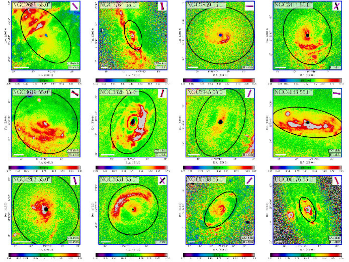
Figure 9: Spiral-like structure (S)-type dusty galaxies. Each tick on the colour-bar indicates median$-5\sigma$, median$-4\sigma$, median$-3\sigma$, median$-2\sigma$, median$-\sigma$, median, median$+\sigma$, median$+2\sigma$, and median$+3\sigma$, respectively. The median and standard deviation values are calculated in the region of 0-1 R_eff, which is shown with the black ellipse. The white scale bar at the bottom corner indicates 1 kpc. On the top-right, we show an illustration of the position angles of the various galaxy components: in purple the H I-disc from Serra et al. (2014); in black the optical-disc from Krajnović et al. (2011); and in red the CO-disc from Alatalo et al. (2013).

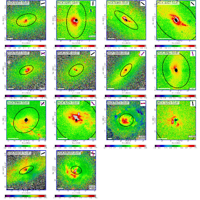
Figure 10: Irregular (Ir)-type dusty galaxies. The colour-bar and other components are similar to that of Fig. 9

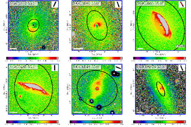
Figure 11: Ring (R)-type dusty galaxies. The colour-bar and other components are similar to that of Fig. 9

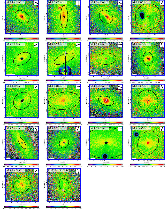
Figure 12: No (N)-type dusty galaxies. The colour-bar and other components are similar to that of Fig. 9

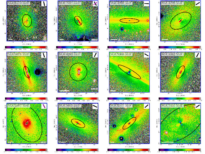
Figure 13: Disc (D)-type dusty galaxies. The colour-bar and other components are similar to that of Fig. 9

Appendix D Figures of individual galaxies

Here, we give the true colour images together with $g^{\prime}-r^{\prime}$ colour and $E(g^{\prime}-r^{\prime})$ colour excess maps of the sample galaxies. The images are the same as Fig. 2. The size of the true colour images is 300$\times$300 arcsec². The colour and colour excess maps in the top panel show the central area with a size of 100$\times$100 arcsec². The maps in the bottom panel are more zoomed-in and show an area with a size of 35$\times$35 arcsec².

If H I is observed in a galaxy, we show column density contours with magenta lines. The H I column density contour levels are given on the true colour images. We note that the H I extends beyond the area shown.

If CO is observed in a galaxy, we show the CO intensity contours with black lines levels in the bottom zoomed-in panel since CO is mostly detected in the inner regions. The CO intensity contour levels are indicated in the same panel.

If a galaxy is classified as dusty, we indicate the dust radius with a white ellipse, which is determined by visual inspection (see Table 3). The white bar in the panels represents 1 kpc spatial size. We also show an illustration of the position angle as in Fig. 1.

Additionally, we show two radial profiles for the sample galaxies. Top: The radial profiles of the $g^{\prime}-r^{\prime}$ colour maps, and the final model obtained in the dust-free colour calculation process (see Appendix A). The red profile with squares and error bars show the median value of the annuli. The solid blue profile shows the final model, which is flattened before 0.5 R_eff and after 3 R_eff. Bottom: Radial profiles of the colour excess maps (blue). The colour excess values are given on the right-y axis, and the corresponding average H I mass density values are given on the left-y axis. If H I or CO is observed in a galaxy, we also show a mass density profile wtih a green or yellow line, respectively.

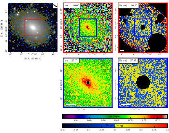
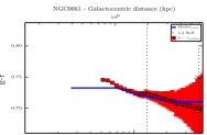
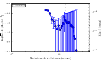
Figure 14: True colour image of NGC 0661 together with $g^{\prime}-r^{\prime}$ colour and $E(g^{\prime}-r^{\prime})$ colour excess maps. All the parameters are the same as in Fig. 2. Bottom-left: The radial profiles of NGC 0661 are similar as in 8.

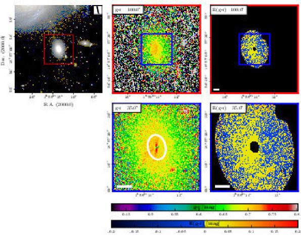
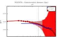
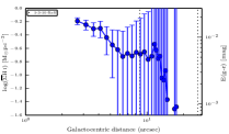
Figure 15: True image, colour map, colour excess map, and the radial profiles of NGC 0770.

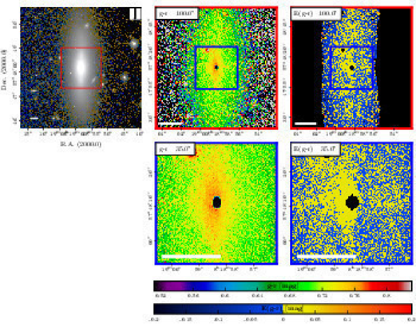
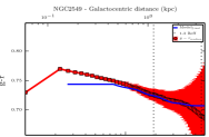
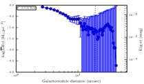
Figure 16: True image, colour map, colour excess map, and the radial profiles of NGC 2549.

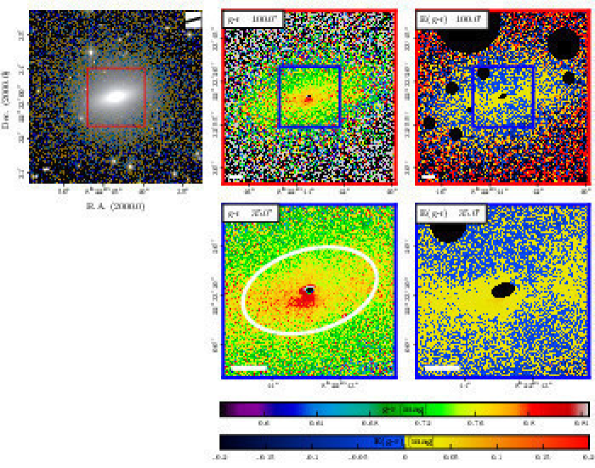
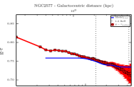
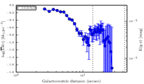
Figure 17: True image, colour map, colour excess map, and the radial profiles of NGC 2577.

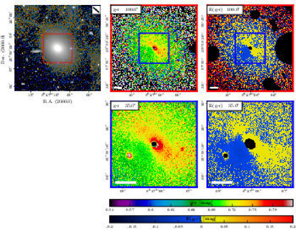
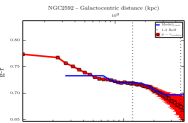
Figure 18: True image, colour map, colour excess map, and the radial profiles of NGC 2592.

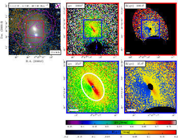
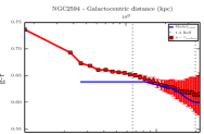
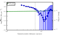
Figure 19: True image, colour map, colour excess map, and the radial profiles of NGC 2594.

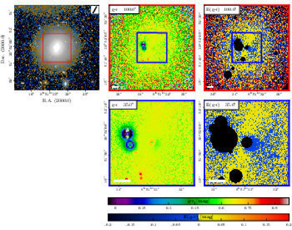
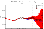
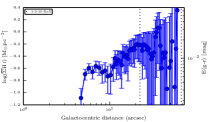
Figure 20: True image, colour map, colour excess map, and the radial profiles of NGC 2679.

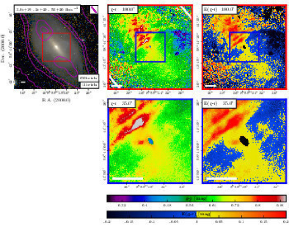
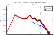
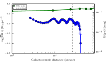
Figure 21: True image, colour map, colour excess map, and the radial profiles of NGC 2685.

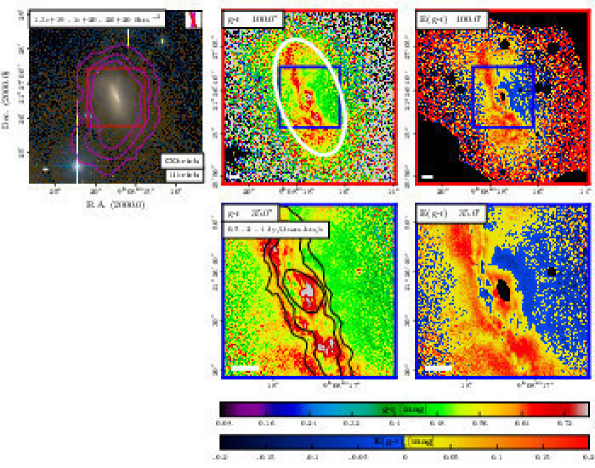
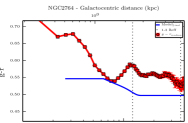
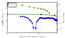
Figure 22: True image, colour map, colour excess map, and the radial profiles of NGC 2764.

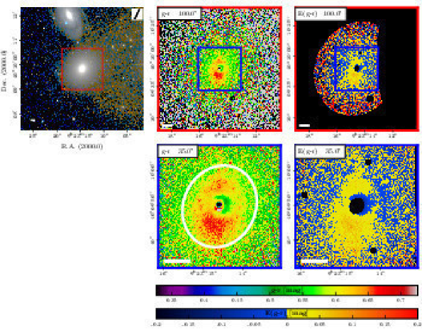
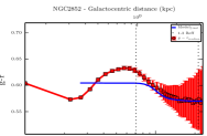
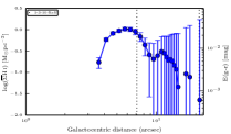
Figure 23: True image, colour map, colour excess map, and the radial profiles of NGC 2852.

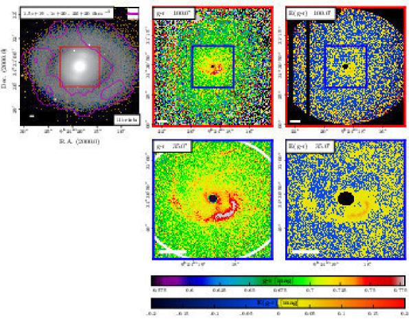
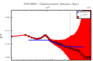
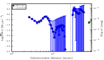
Figure 24: True image, colour map, colour excess map, and the radial profiles of NGC 2859.

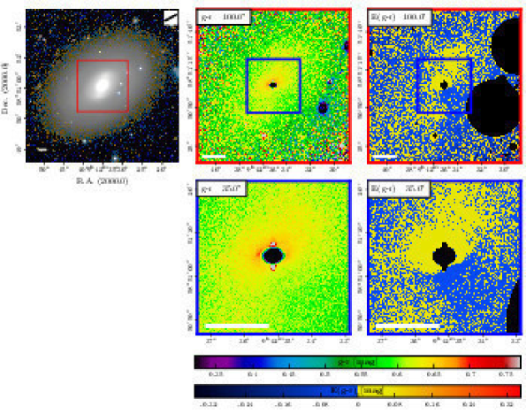
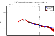
Figure 25: True image, colour map, colour excess map, and the radial profiles of NGC 2950.

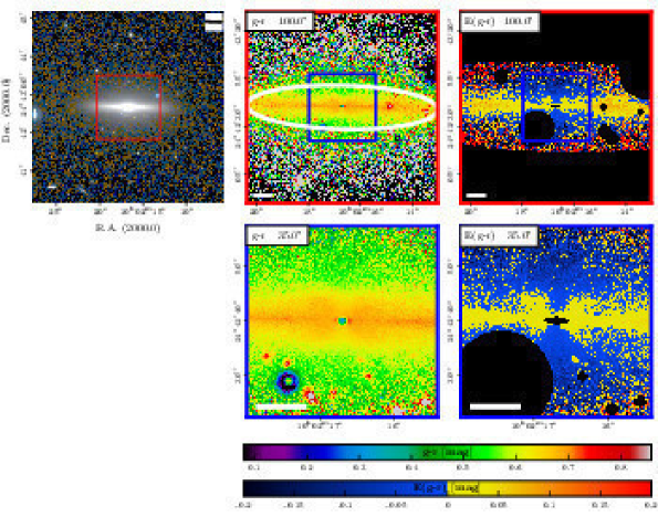
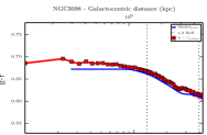
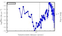
Figure 26: True image, colour map, colour excess map, and the radial profiles of NGC 3098.

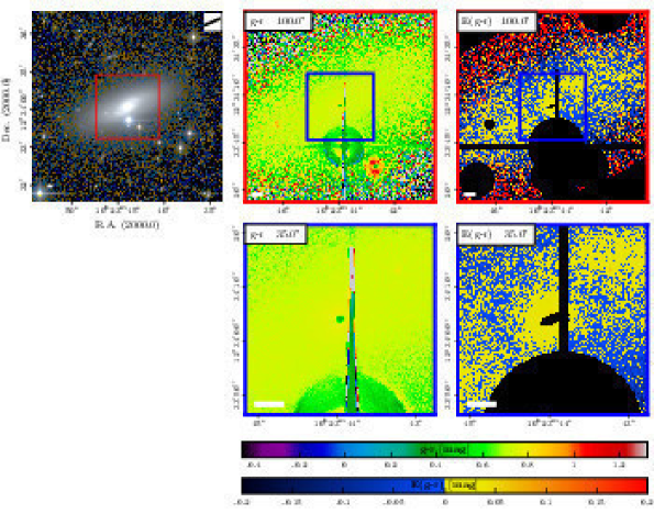
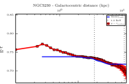
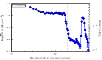
Figure 27: True image, colour map, colour excess map, and the radial profiles of NGC 3230.

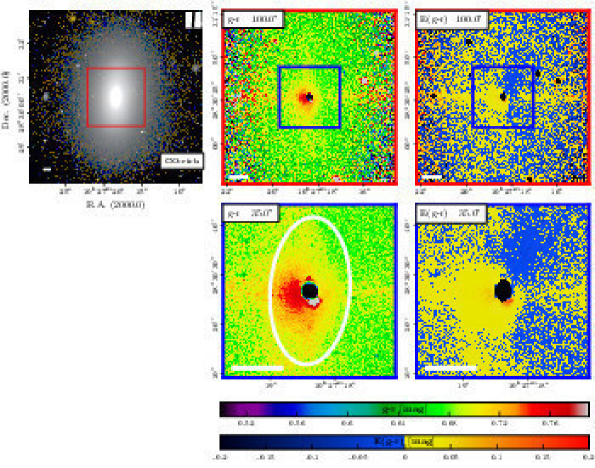
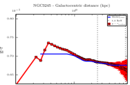
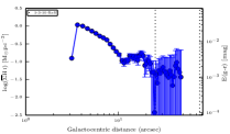
Figure 28: True image, colour map, colour excess map, and the radial profiles of NGC 3245.

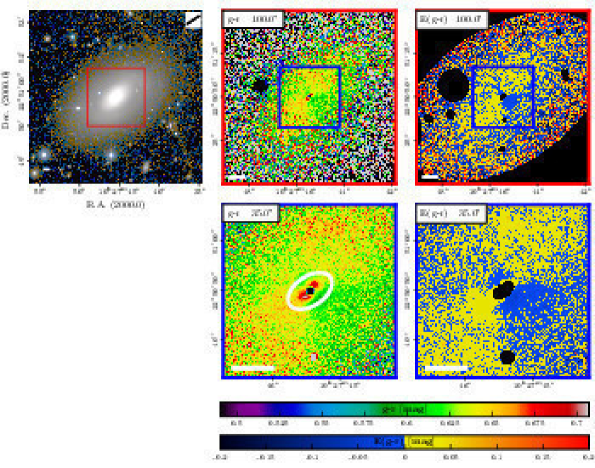
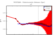
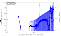
Figure 29: True image, colour map, colour excess map, and the radial profiles of NGC 3248.

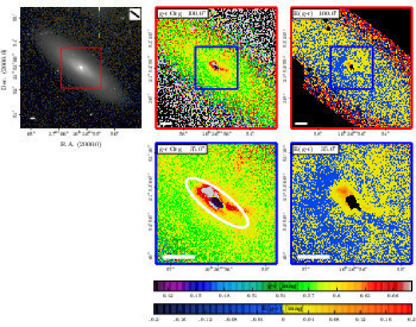
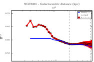
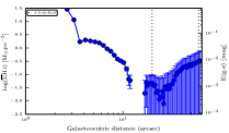
Figure 30: True image, colour map, colour excess map, and the radial profiles of NGC 3301.

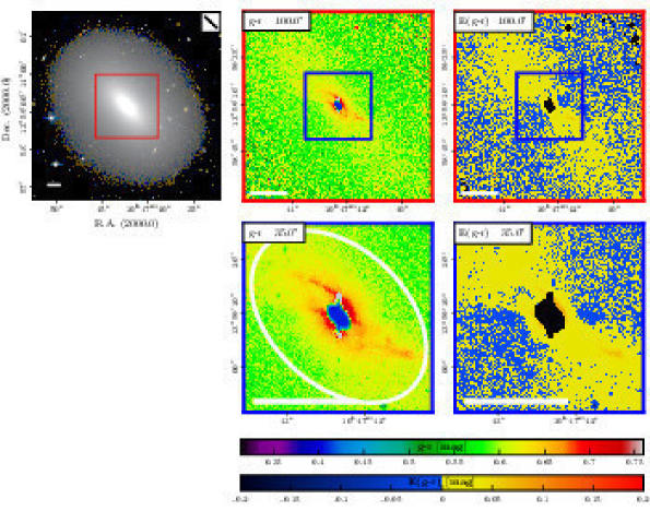
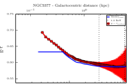
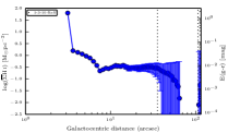
Figure 31: True image, colour map, colour excess map, and the radial profiles of NGC 3377.

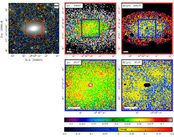
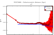
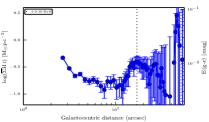
Figure 32: True image, colour map, colour excess map, and the radial profiles of NGC 3400.

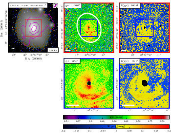
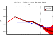
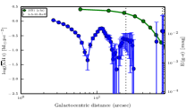
Figure 33: True image, colour map, colour excess map, and the radial profiles of NGC 3414.

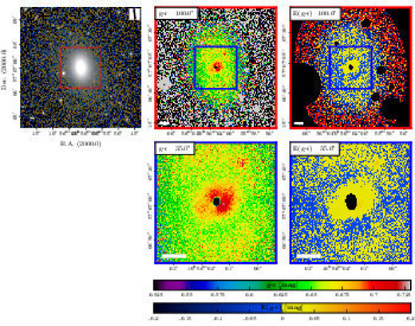
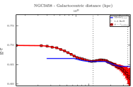
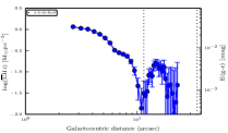
Figure 34: True image, colour map, colour excess map, and the radial profiles of NGC 3458.

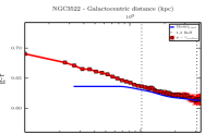
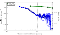
Figure 35: True image, colour map, colour excess map, and the radial profiles of NGC 3522.

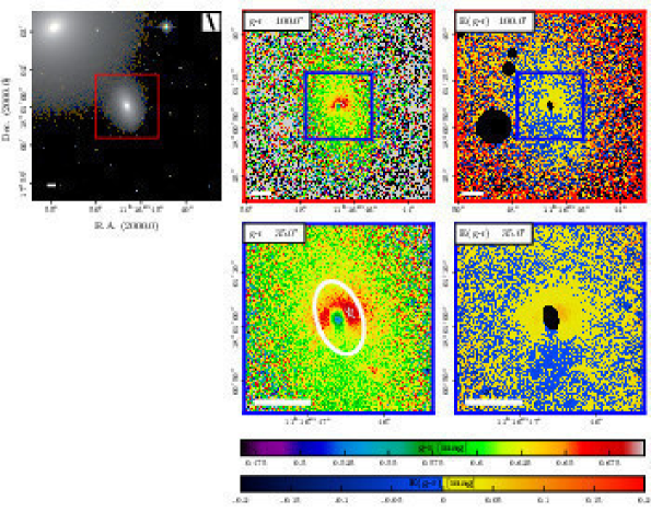
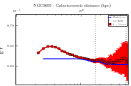
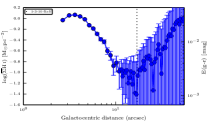
Figure 36: True image, colour map, colour excess map, and the radial profiles of NGC 3605.

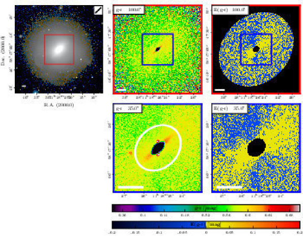
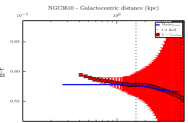
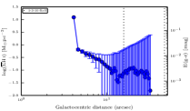
Figure 37: True image, colour map, colour excess map, and the radial profiles of NGC 3610.

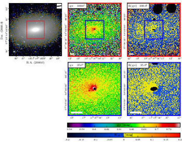
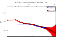
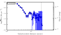
Figure 38: True image, colour map, colour excess map, and the radial profiles of NGC 3613.

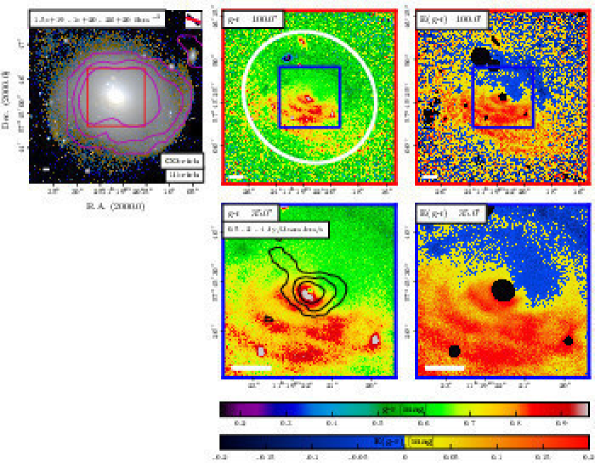
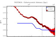
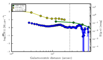
Figure 39: True image, colour map, colour excess map, and the radial profiles of NGC 3619.

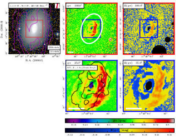
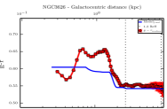
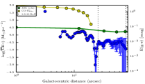
Figure 40: True image, colour map, colour excess map, and the radial profiles of NGC 3626.

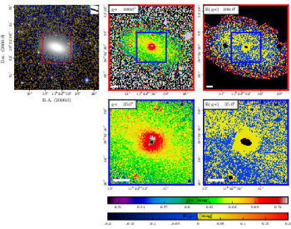
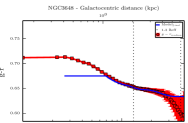
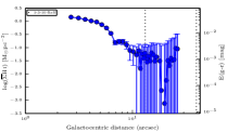
Figure 41: True image, colour map, colour excess map, and the radial profiles of NGC 3648.

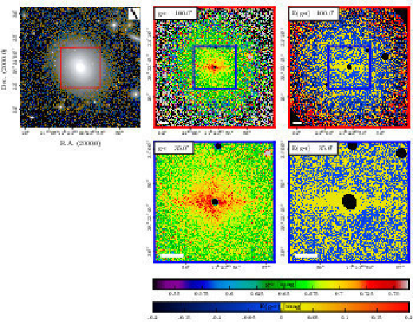
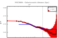
Figure 42: True image, colour map, colour excess map, and the radial profiles of NGC 3658.

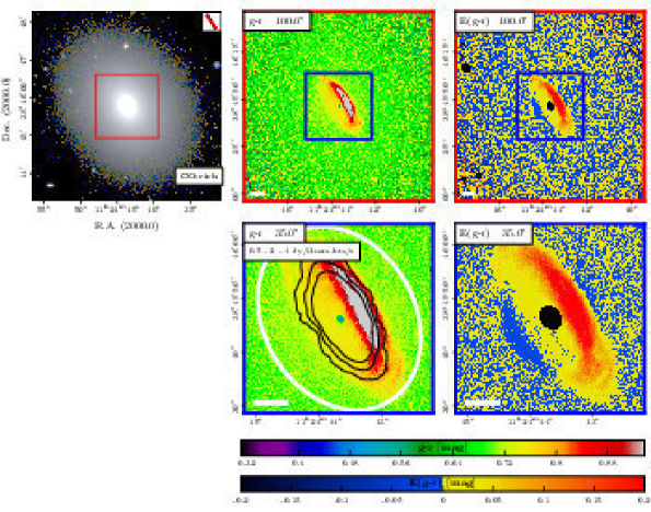
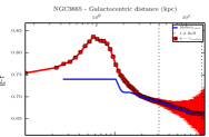
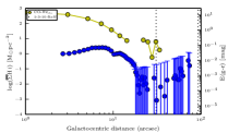
Figure 43: True image, colour map, colour excess map, and the radial profiles of NGC 3665.

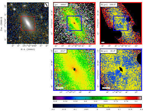
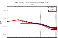
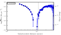
Figure 44: True image, colour map, colour excess map, and the radial profiles of NGC 3674.

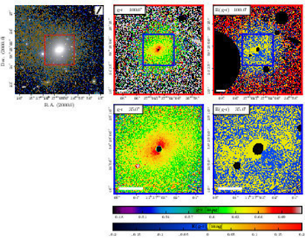
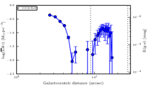
Figure 45: True image, colour map, colour excess map, and the radial profiles of NGC 3757.

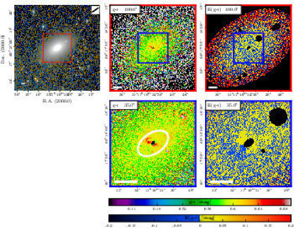
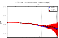
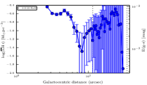
Figure 46: True image, colour map, colour excess map, and the radial profiles of NGC 3796.

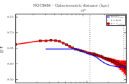
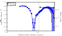
Figure 47: True image, colour map, colour excess map, and the radial profiles of NGC 3838.

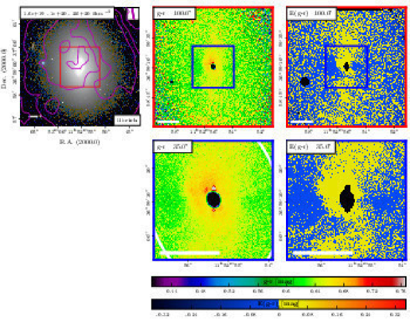
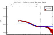
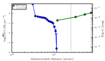
Figure 48: True image, colour map, colour excess map, and the radial profiles of NGC 3941.

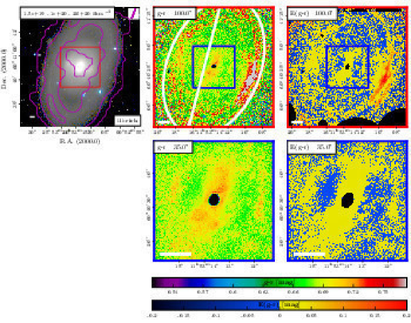
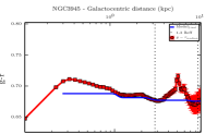
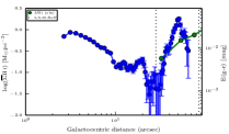
Figure 49: True image, colour map, colour excess map, and the radial profiles of NGC 3945.

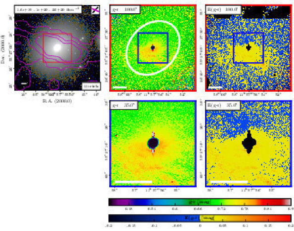
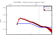
Figure 50: True image, colour map, colour excess map, and the radial profiles of NGC 3998.

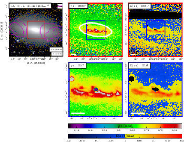
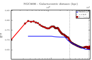
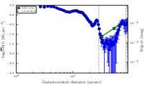
Figure 51: True image, colour map, colour excess map, and the radial profiles of NGC 4036.

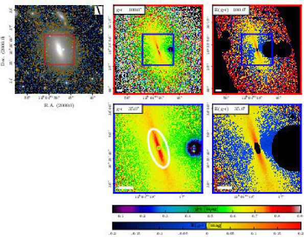
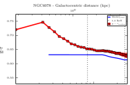
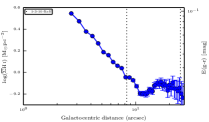
Figure 52: True image, colour map, colour excess map, and the radial profiles of NGC 4078.

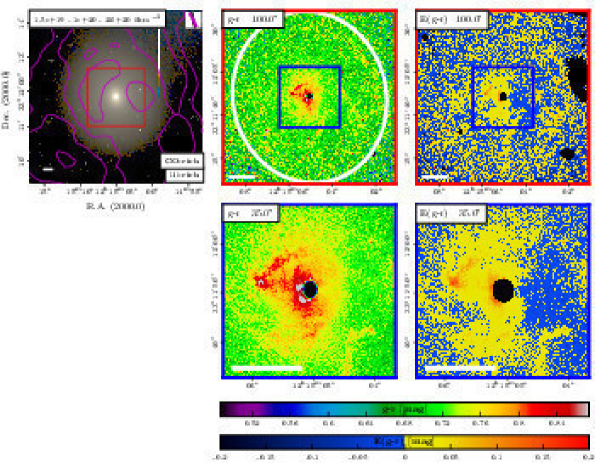
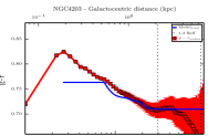
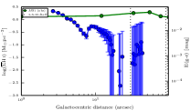
Figure 53: True image, colour map, colour excess map, and the radial profiles of NGC 4203.

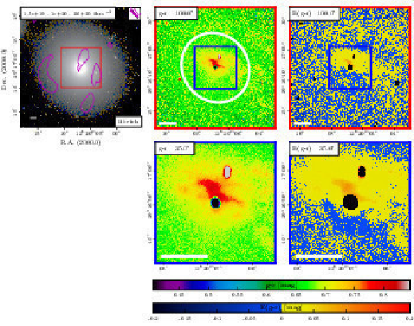
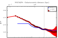
Figure 54: True image, colour map, colour excess map, and the radial profiles of NGC 4278.

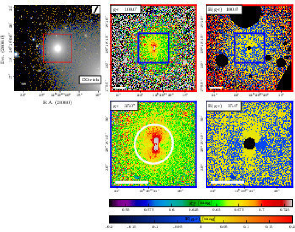
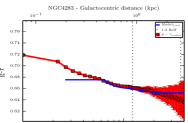
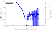
Figure 55: True image, colour map, colour excess map, and the radial profiles of NGC 4283.

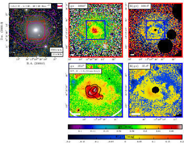
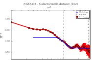
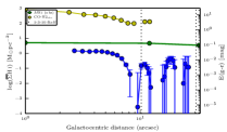
Figure 56: True image, colour map, colour excess map, and the radial profiles of NGC 5173.

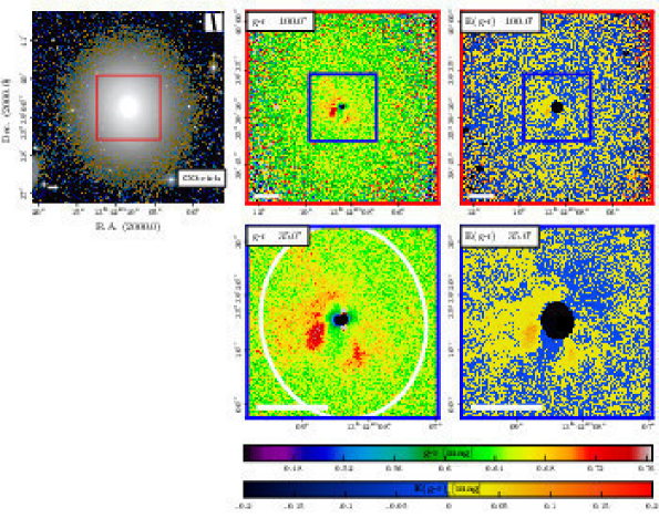
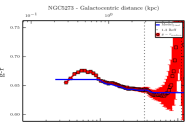
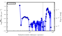
Figure 57: True image, colour map, colour excess map, and the radial profiles of NGC 5273.

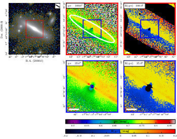
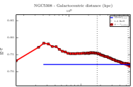
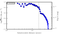
Figure 58: True image, colour map, colour excess map, and the radial profiles of NGC 5308.

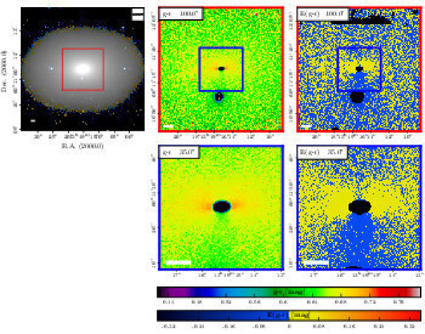
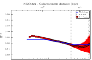
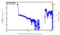
Figure 59: True image, colour map, colour excess map, and the radial profiles of NGC 5322.

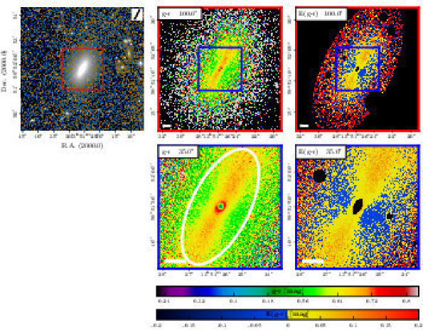
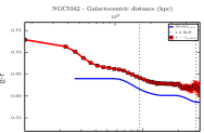
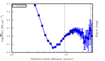
Figure 60: True image, colour map, colour excess map, and the radial profiles of NGC 5342.

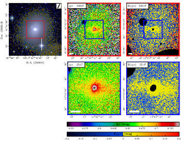
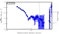
Figure 61: True image, colour map, colour excess map, and the radial profiles of NGC 5473.

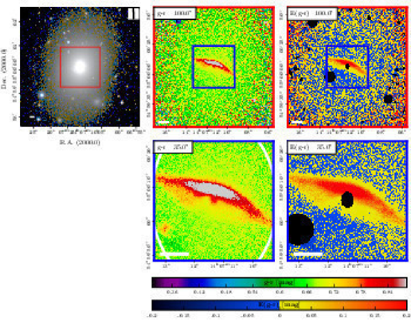
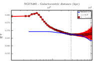
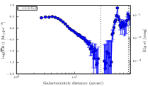
Figure 62: True image, colour map, colour excess map, and the radial profiles of NGC 5485.

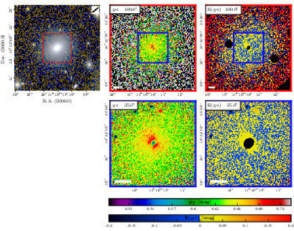
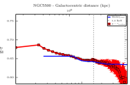
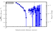
Figure 63: True image, colour map, colour excess map, and the radial profiles of NGC 5500.

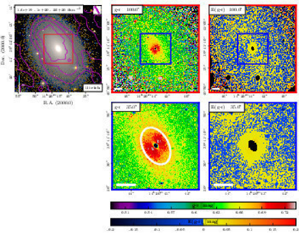
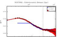
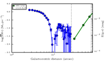
Figure 64: True image, colour map, colour excess map, and the radial profiles of NGC 5582.

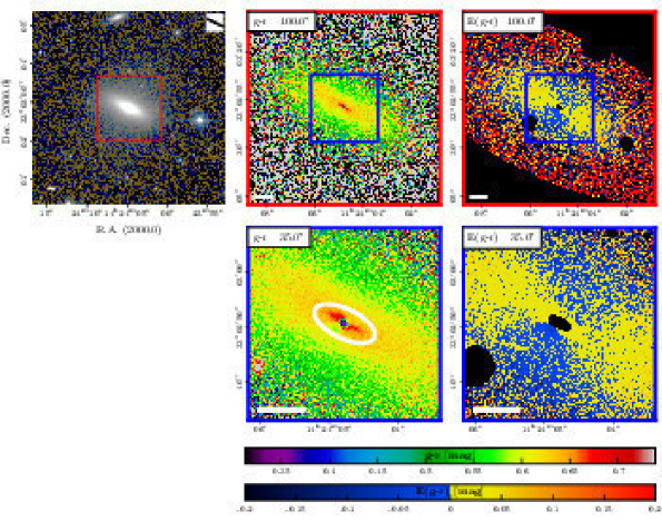
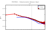
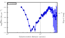
Figure 65: True image, colour map, colour excess map, and the radial profiles of NGC 5611.

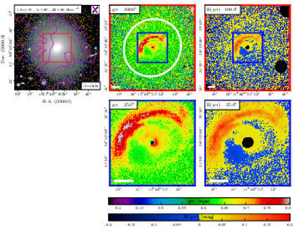
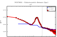
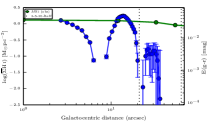
Figure 66: True image, colour map, colour excess map, and the radial profiles of NGC 5631.

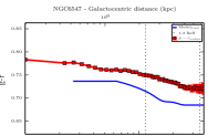
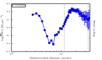
Figure 67: True image, colour map, colour excess map, and the radial profiles of NGC 6547.

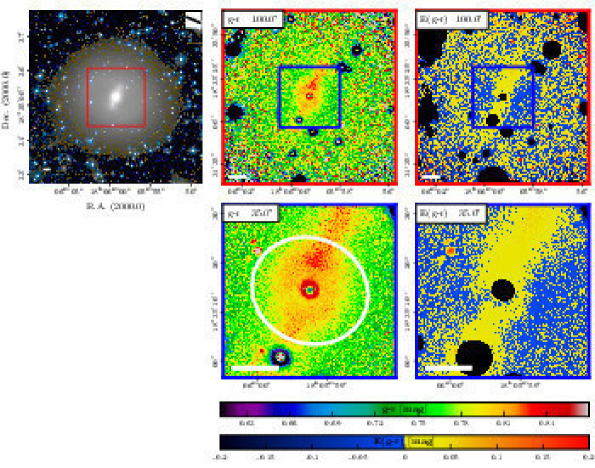
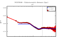
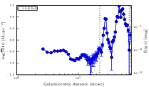
Figure 68: True image, colour map, colour excess map, and the radial profiles of NGC 6548.

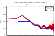
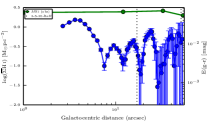
Figure 69: True image, colour map, colour excess map, and the radial profiles of NGC 6798.

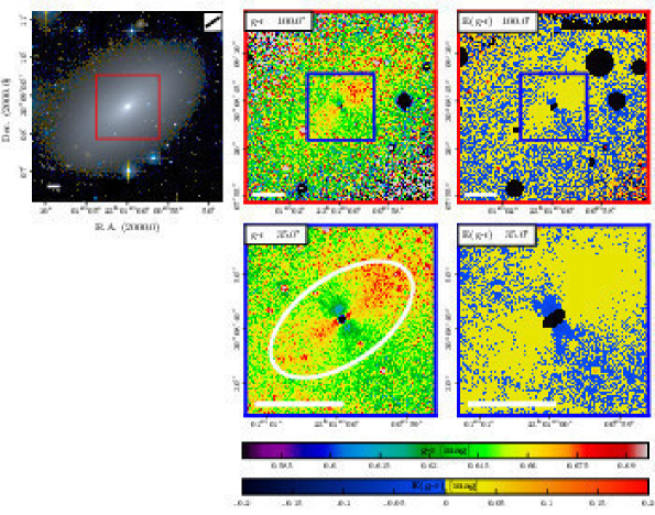
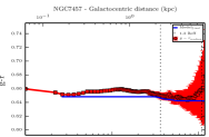
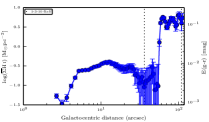
Figure 70: True image, colour map, colour excess map, and the radial profiles of NGC 7457.

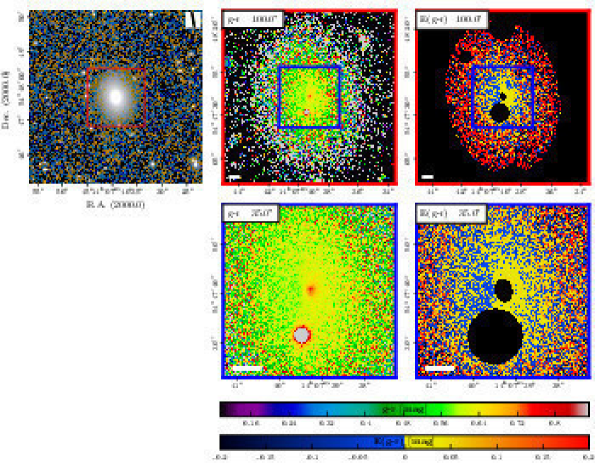
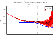
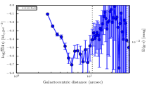
Figure 71: True image, colour map, colour excess map, and the radial profiles of PGC 050395.

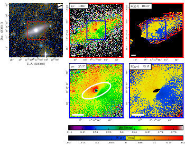
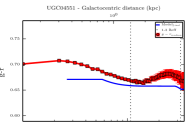
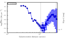
Figure 72: True image, colour map, colour excess map, and the radial profiles of UGC 04551.

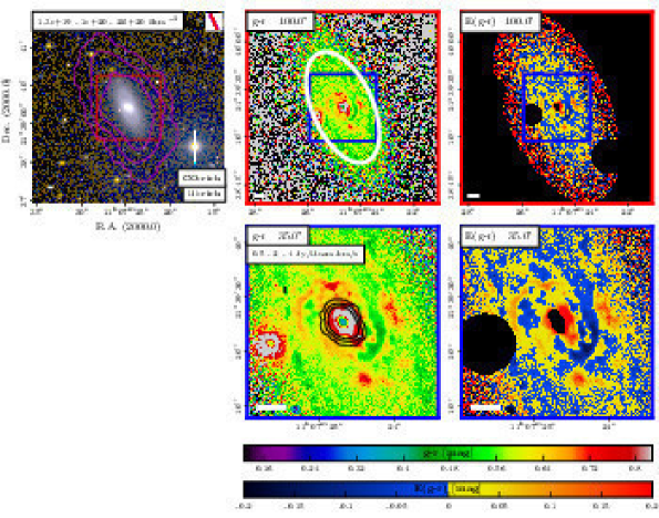
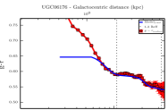
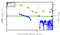
Figure 73: True image, colour map, colour excess map, and the radial profiles of UGC 06167.

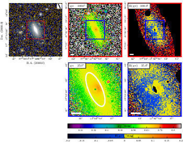
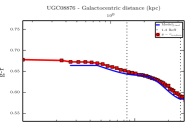
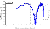
Figure 74: True image, colour map, colour excess map, and the radial profiles of UGC 08867.

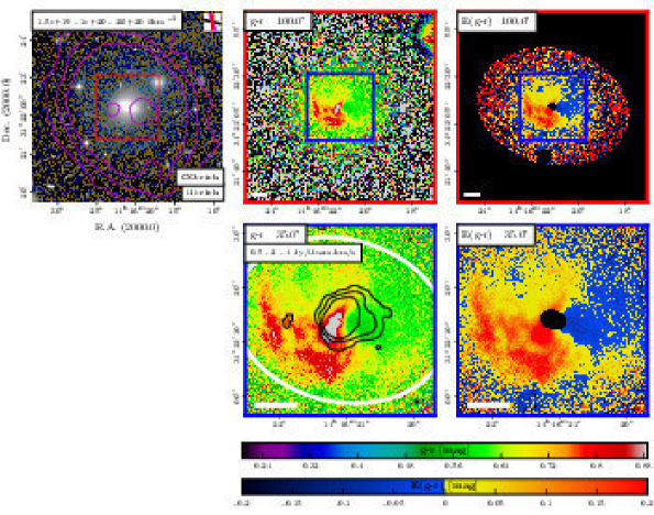
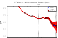
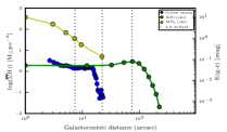
Figure 75: True image, colour map, colour excess map, and the radial profiles of UGC 09519.

References

- Alatalo et al. (2013) Alatalo, K., Davis, T. A., Bureau, M., et al. 2013, MNRAS, 432, 1796
- Bassett et al. (2017) Bassett, R., Bekki, K., Cortese, L., et al. 2017, MNRAS, 470, 1991
- Bernardi et al. (2005) Bernardi, M., Sheth, R. K., Nichol, R. C., Schneider, D. P., & Brinkmann, J. 2005, AJ, 129, 61
- Bertin (2012) Bertin, E. 2012, in Astronomical Society of the Pacific Conference Series, Vol. 461, Astronomical Data Analysis Software and Systems XXI, ed. P. Ballester, D. Egret, & N. P. F. Lorente, 263
- Bertin & Arnouts (1996) Bertin, E. & Arnouts, S. 1996, A&AS, 117, 393
- Bohlin et al. (1978) Bohlin, R. C., Savage, B. D., & Drake, J. F. 1978, ApJ, 224, 132
- Bregman et al. (1998) Bregman, J. N., Snider, B. A., Grego, L., & Cox, C. V. 1998, ApJ, 499, 670
- Bruzual & Charlot (2003) Bruzual, G. & Charlot, S. 2003, MNRAS, 344, 1000
- Bundy et al. (2015) Bundy, K., Bershady, M. A., Law, D. R., et al. 2015, ApJ, 798, 7
- Cappellari et al. (2011a) Cappellari, M., Emsellem, E., Krajnović, D., et al. 2011a, MNRAS, 413, 813
- Cappellari et al. (2011b) Cappellari, M., Emsellem, E., Krajnović, D., et al. 2011b, MNRAS, 416, 1680
- Cappellari et al. (2013) Cappellari, M., Scott, N., Alatalo, K., et al. 2013, MNRAS, 432, 1709
- Carollo et al. (1997) Carollo, C. M., Franx, M., Illingworth, G. D., & Forbes, D. A. 1997, ApJ, 481, 710
- Crocker et al. (2011) Crocker, A. F., Bureau, M., Young, L. M., & Combes, F. 2011, MNRAS, 410, 1197
- Croom et al. (2012) Croom, S. M., Lawrence, J. S., Bland-Hawthorn, J., et al. 2012, MNRAS, 421, 872
- Davis et al. (2013) Davis, T. A., Alatalo, K., Bureau, M., et al. 2013, MNRAS, 429, 534
- Davis et al. (2011) Davis, T. A., Alatalo, K., Sarzi, M., et al. 2011, MNRAS, 417, 882
- Davis et al. (2015) Davis, T. A., Rowlands, K., Allison, J. R., et al. 2015, MNRAS, 449, 3503
- di Serego Alighieri et al. (2013) di Serego Alighieri, S., Bianchi, S., Pappalardo, C., et al. 2013, A&A, 552, A8
- Disney et al. (1989) Disney, M., Davies, J., & Phillipps, S. 1989, MNRAS, 239, 939
- Draine & Li (2007) Draine, B. T. & Li, A. 2007, ApJ, 657, 810
- Duc et al. (2015) Duc, P.-A., Cuillandre, J.-C., Karabal, E., et al. 2015, MNRAS, 446, 120
- Duc et al. (2014) Duc, P.-A., Paudel, S., McDermid, R. M., et al. 2014, MNRAS, 440, 1458
- Emsellem et al. (2011) Emsellem, E., Cappellari, M., Krajnović, D., et al. 2011, MNRAS, 414, 888
- Emsellem et al. (2007) Emsellem, E., Cappellari, M., Krajnović, D., et al. 2007, MNRAS, 379, 401
- Ferrari et al. (1999) Ferrari, F., Pastoriza, M. G., Macchetto, F., & Caon, N. 1999, A&AS, 136, 269
- Finkelman et al. (2012) Finkelman, I., Brosch, N., Funes, J. G., et al. 2012, MNRAS, 422, 1384
- Ford et al. (1997) Ford, H., Tsvetanov, Z., Ferrarese, L., et al. 1997, in Astronomical Society of the Pacific Conference Series, Vol. 121, IAU Colloq. 163: Accretion Phenomena and Related Outflows, ed. D. T. Wickramasinghe, G. V. Bicknell, & L. Ferrario, 620
- Franx et al. (1989) Franx, M., Illingworth, G., & Heckman, T. 1989, AJ, 98, 538
- Gavazzi et al. (2018) Gavazzi, G., Consolandi, G., Pedraglio, S., et al. 2018, A&A, 611, A28
- Geréb et al. (2016) Geréb, K., Catinella, B., Cortese, L., et al. 2016, MNRAS, 462, 382
- Gomes et al. (2016) Gomes, J. M., Papaderos, P., Kehrig, C., et al. 2016, A&A, 588, A68
- Goudfrooij et al. (1994) Goudfrooij, P., de Jong, T., Hansen, L., & Norgaard-Nielsen, H. U. 1994, MNRAS, 271, 833
- Józsa et al. (2009) Józsa, G. I. G., Oosterloo, T. A., Morganti, R., Klein, U., & Erben, T. 2009, A&A, 494, 489
- Karabal et al. (2017) Karabal, E., Duc, P.-A., Kuntschner, H., et al. 2017, A&A, 601, A86
- Kaviraj et al. (2007) Kaviraj, S., Schawinski, K., Devriendt, J. E. G., et al. 2007, ApJS, 173, 619
- Kaviraj et al. (2012) Kaviraj, S., Ting, Y.-S., Bureau, M., et al. 2012, MNRAS, 423, 49
- Knapp et al. (1989) Knapp, G. R., Guhathakurta, P., Kim, D.-W., & Jura, M. A. 1989, ApJS, 70, 329
- Kokusho et al. (2017) Kokusho, T., Kaneda, H., Bureau, M., et al. 2017, A&A, 605, A74
- Kokusho et al. (2019) Kokusho, T., Kaneda, H., Bureau, M., et al. 2019, A&A, 622, A87
- Kormendy & Bender (2012) Kormendy, J. & Bender, R. 2012, ApJS, 198, 2
- Krajnović et al. (2013) Krajnović, D., Alatalo, K., Blitz, L., et al. 2013, MNRAS, 432, 1768
- Krajnović et al. (2011) Krajnović, D., Emsellem, E., Cappellari, M., et al. 2011, MNRAS, 414, 2923
- Kuntschner et al. (2010) Kuntschner, H., Emsellem, E., Bacon, R., et al. 2010, MNRAS, 408, 97
- Lauer et al. (1995) Lauer, T. R., Ajhar, E. A., Byun, Y.-I., et al. 1995, AJ, 110, 2622
- Lauer et al. (2005) Lauer, T. R., Faber, S. M., Gebhardt, K., et al. 2005, AJ, 129, 2138
- Laurikainen et al. (2011) Laurikainen, E., Salo, H., Buta, R., & Knapen, J. H. 2011, MNRAS, 418, 1452
- Martini et al. (2013) Martini, P., Dicken, D., & Storchi-Bergmann, T. 2013, ApJ, 766, 121
- McDermid et al. (2015) McDermid, R. M., Alatalo, K., Blitz, L., et al. 2015, MNRAS, 448, 3484
- Morganti et al. (2006) Morganti, R., de Zeeuw, P. T., Oosterloo, T. A., et al. 2006, MNRAS, 371, 157
- Muñoz et al. (2014) Muñoz, R. P., Puzia, T. H., Lançon, A., et al. 2014, ApJS, 210, 4
- Oosterloo et al. (2010) Oosterloo, T., Morganti, R., Crocker, A., et al. 2010, MNRAS, 409, 500
- Oosterloo et al. (2007) Oosterloo, T. A., Morganti, R., Sadler, E. M., van der Hulst, T., & Serra, P. 2007, A&A, 465, 787
- Orellana et al. (2017) Orellana, G., Nagar, N. M., Elbaz, D., et al. 2017, A&A, 602, A68
- Pahre et al. (2004) Pahre, M. A., Ashby, M. L. N., Fazio, G. G., & Willner, S. P. 2004, ApJS, 154, 229
- Patil et al. (2007) Patil, M. K., Pandey, S. K., Sahu, D. K., & Kembhavi, A. 2007, A&A, 461, 103
- Paturel et al. (2003) Paturel, G., Petit, C., Prugniel, P., et al. 2003, A&A, 412, 45
- Peletier et al. (1999) Peletier, R. F., Balcells, M., Davies, R. L., et al. 1999, MNRAS, 310, 703
- Peletier et al. (1990) Peletier, R. F., Davies, R. L., Illingworth, G. D., Davis, L. E., & Cawson, M. 1990, AJ, 100, 1091
- Peletier et al. (2012) Peletier, R. F., Kutdemir, E., van der Wolk, G., et al. 2012, MNRAS, 419, 2031
- Rampazzo et al. (2005) Rampazzo, R., Annibali, F., Bressan, A., et al. 2005, A&A, 433, 497
- Sadler & Gerhard (1985) Sadler, E. M. & Gerhard, O. E. 1985, MNRAS, 214, 177
- Sánchez et al. (2012) Sánchez, S. F., Kennicutt, R. C., Gil de Paz, A., et al. 2012, A&A, 538, A8
- Sarzi et al. (2006) Sarzi, M., Falcón-Barroso, J., Davies, R. L., et al. 2006, MNRAS, 366, 1151
- Schlafly & Finkbeiner (2011) Schlafly, E. F. & Finkbeiner, D. P. 2011, ApJ, 737, 103
- Serra et al. (2012) Serra, P., Oosterloo, T., Morganti, R., et al. 2012, MNRAS, 422, 1835
- Serra et al. (2014) Serra, P., Oser, L., Krajnović, D., et al. 2014, MNRAS, 444, 3388
- Serra & Trager (2007) Serra, P. & Trager, S. C. 2007, MNRAS, 374, 769
- Simões Lopes et al. (2007) Simões Lopes, R. D., Storchi-Bergmann, T., de Fátima Saraiva, M., & Martini, P. 2007, ApJ, 655, 718
- Smith et al. (2012) Smith, M. W. L., Gomez, H. L., Eales, S. A., et al. 2012, ApJ, 748, 123
- Springob et al. (2005) Springob, C. M., Haynes, M. P., Giovanelli, R., & Kent, B. R. 2005, ApJS, 160, 149
- Temi et al. (2007) Temi, P., Brighenti, F., & Mathews, W. G. 2007, ApJ, 660, 1215
- Trager et al. (2000) Trager, S. C., Faber, S. M., Worthey, G., & González, J. J. 2000, AJ, 119, 1645
- Tran et al. (2001) Tran, H. D., Tsvetanov, Z., Ford, H. C., et al. 2001, AJ, 121, 2928
- van Dokkum & Franx (1995) van Dokkum, P. G. & Franx, M. 1995, AJ, 110, 2027
- van Driel & van Woerden (1991) van Driel, W. & van Woerden, H. 1991, A&A, 243, 71
- Viaene et al. (2015) Viaene, S., De Geyter, G., Baes, M., et al. 2015, A&A, 579, A103
- Weijmans et al. (2014) Weijmans, A.-M., de Zeeuw, P. T., Emsellem, E., et al. 2014, MNRAS, 444, 3340
- Yıldız et al. (2015) Yıldız, M. K., Serra, P., Oosterloo, T. A., et al. 2015, MNRAS, 451, 103
- Yıldız et al. (2017) Yıldız, M. K., Serra, P., Peletier, R. F., Oosterloo, T. A., & Duc, P.-A. 2017, MNRAS, 464, 329
- Young (2002) Young, L. M. 2002, AJ, 124, 788
- Young et al. (2011) Young, L. M., Bureau, M., Davis, T. A., et al. 2011, MNRAS, 414, 940