|
|
Effect of the interaction strength and anisotropy on the diffusio-phoresis of spherical colloids |
| Jiachen Wei,a,b Simón Ramírez-Hinestrosa,b Jure Dobnikar, b,c,d∗ and Daan Frenkelb† | |
|
|
Gradients in temperature, concentration or electrostatic potential cannot exert forces on a bulk fluid; they can, however, exert forces on a fluid in a microscopic boundary layer surrounding a (nano)colloidal solute, resulting in so-called phoretic flow. Here we present a simulation study of phoretic flow around a spherical colloid held fixed in a concentration gradient. We show that the resulting flow velocity depends non-monotonically on the strength of the colloid-fluid interaction. The reason for this non-monotonic dependence is that solute particles are effectively trapped in a shell around the colloid and cannot contribute to diffusio-phoresis. We also observe that the flow depends sensitively on the anisotropy of solute-colloid interaction. |
1 Introduction
The term “phoresis” covers a class of transport phenomena that are generated by thermodynamic gradients. Phoretic transport can be induced by gradients in chemical potential 1, 2, 3, 4, 5, 6, 7, 8, 9, 10, 11, 12, 13, 14, temperature 15, 16, 17, 18, 19, 20, 21, 22, 23, 24, 25, 26, 27 or electrostatic potential 28, 29, 30, 31, 32. Electrophoresis is commonly used to separate bio-molecules, but other phoretic phenomena could, in principle, be used for the same purpose. In this paper, we consider the challenges involved in developing separation techniques based on diffusio-phoresis.
The conventional theoretical description of phoretic transport combines a local thermodynamics description of the fluid around a colloidal particle with Stokesian hydrodynamics 33, 2, 6, 14, 34, 35. Whilst such a continuum description is usually adequate for electrophoresis, it is less applicable in the case of diffusio- and thermo-phoresis, where the characteristic length-scales are often too small to justify local hydrodynamics/thermodynamics. In particular, the continuum picture fails to account for ordering on an atomistic scale near an interface 36, 37, even though its predictions are qualitatively similar to those obtained by molecular simulation 38. As experiments move increasingly to the nano-scale 39, 40, 41, and as direct simulations are becoming feasible 42, we are now in a position to explore the diffusion-phoretic transport of uncharged (nano)colloidal particles.
The most straightforward method to simulate phoresis is to impose an explicit gradient in the concentration or temperature 38, 43, 37, 19. This approach is less suited for systems with periodic boundary conditions. However, as shown in recent papers, the gradient can also be imposed as an external force acting on the chemical identity (in the case of diffusio-phoresis) or the excess enthalpy (in the case of thermophoresis) of individual particles 44, 45.
In the present paper we investigate the dependence of the diffusio-phoretic mobility on the strength and anisotropy of the solute-colloid interaction. In addition, we consider the effect of different hydrodynamic boundary conditions. In the next section we introduce the model and the simulation methods and then proceed to analyze the results of the simulations.
2 Simulation method
2.1 Model
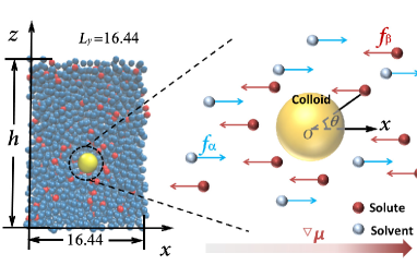
We performed Molecular Dynamics (MD) simulations of diffusio-phoresis in a system with a single colloidal particle () immersed in a fluid comprising solvent () and solute () particles. All fluid particles were assumed to be of the same diameter , which was used as a unit of length. The diameter of the colloidal particle was taken to be . The system dimensions were , where the box height was varied to keep the pressure constant. We applied periodic boundary conditions and measured the velocity of the fluid flow, whilst keeping the colloidal particle fixed at the origin.
We assumed interaction potentials of the form
| (1) |
where denotes an isotropic short range potential , while denotes a possible anisotropic interaction between colloid and solutes. We assume that the fluid particles interact isotropically among themselves and that the only interaction with angular dependence is that between the colloid and the solute particles. Therefore, the only non-vanishing pre-factor controlling the strength of the anisotropy is . The choice of the short-ranged isotropic interaction potential was dictated by computational convenience. We start from a recently introduced generic, short-ranged, attractive pair potential 46:
where is chosen such that the minimum value of equals -1:
| (2) |
From this pair potential, we construct a short-ranged potential that has an adjustable well depth :
| (3) |
Indices denote the type of the particles: , is the distance where the potential crosses zero, denotes the cutoff radius (we choose for fluid–fluid, and for fluid–colloid interactions), the location of the potential minimum, and controls the depth of the potential well.
In what follows, the strength of the interaction between all fluid species as our unit of energy: . Furthermore, we fix the solvent-colloid interaction strengths, , and vary the solute-colloid interaction ). The overview of the interaction parameters is shown in the Table 1.
| solvent-solvent | |||
|---|---|---|---|
| solvent-solute | |||
| solute-solute | |||
| solvent-colloid | |||
| solute-colloid |
The minimum of the interaction potential is located at:
| (4) |
An advantage of this model potential is that the potential and its first derivative vanish at 46. However, for the solute-colloid interaction, the force is discontinuous for , although the potential is continuous.
When studying the effect of anisotropic colloid-solute interactions, we decompose these interactions in terms of Legendre polynomials :
| (5) |
where denotes the angle between symmetry axis of the colloidal particle and the vector joining the centers of mass of the colloid and a solute particle (see Fig. 1). The advantage of using a Legendre-polynomial decomposition is that, in the limit of weak anisotropic interactions, the integrated excess density vanishes for all .
As shown in Fig. 1, we represent the effect of a concentration (or chemical-potential) gradient 44, 43 by applying opposing external “color" forces on the solvent and solute particles:
| (6) |
where is the chemical potential and the number density. The reason for carrying out a simulation with color forces, rather than the corresponding explicit concentration gradients, is twofold. First of all, as in the case of simulations of systems in electrical fields, it is often better to impose a constant field that is compatible with the periodic boundary conditions, than to impose a periodic charge density that would locally lead to the same field.
The second reason is specific for phoretic transport: in principle, we should carry out these simulations under conditions where the phoretic flow velocity is so small that the concentration profile is not perturbed by the flow (the limit of vanishing Peclet number). With explicit concentration gradients, the relevant Peclet number is , where is te average phoretic flow velocity, is the system size and is the diffusion coefficient of the solutes/solvent molecules. However, with imposed color forces, the relevant Peclet number is , where is the colloidal diameter. As, typically, , the Peclet number for simulations with color forces is much smaller than the corresponding number in the presence of explicit concentration gradients. As shown in the SI, simulations with an explicit concentration gradient 43, in a box with the position of the colloidal particle fixed at the origin, lead to a strongly non-linear (in fact: exponential) concentration profile at flow velocities where no such problem occurs if we impose color forces.
2.2 Simulation Details
All simulations were performed at constant , and , with the number of particles fixed at , and the temperature at . The length of the simulation time step was , and a Nosé-Hoover thermostat with a time constant of was used to control the temperature. Here and in what follows, we use reduced units, based on the , and (mass) of the solvent particles.
All initial configurations were prepared by placing solvent particles on a low-density FCC crystal lattice. randomly chosen solvent particles were then replaced with solute particles, where is the volume of the simulation box. The system was then compressed in direction and quenched to the desired pressure (). The identities of solvent and solute particles in the bulk (i.e. far away from the colloidal particle) were allowed to interchange every simulation steps to keep the solute density constant at for at least simulation steps. Color forces along the -direction were then applied to the solvent and solute particles. Subsequently, a run of at least steps was performed to obtain the flow rate and density profile, which were collected by averaging over output configurations separated by simulation steps. The applied color forces correspond to a solute concentration gradient of .
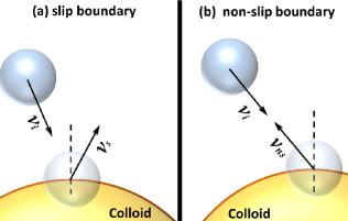
Integrating the MD equations of motion with the Verlet algorithm, which conserves the tangential velocity of a solvent/solute particle when interacting with the colloid. As a result, this situation corresponds to a “slip” boundary condition (Fig. 2(a)). To implement non-slip boundary conditions, we reverse the velocity of the solvent/particle at the distance (Fig. 2(b)). In our simulations, we chose , where refers to both solvent and solute particles. Note, however, that the definition of non-slip boundary conditions is not unambiguous for systems with a continuous colloid-fluid interaction.
3 Result and discussion
3.1 Isotropic interaction
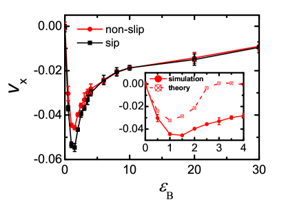
Fig. 3 shows the diffusio-phoretic flow past a colloid that interacts with the solvent and solute particles with isotropic () potential specified in the previous section. For , the magnitude of the velocity in the direction of phoretic motion obtained from simulations, , increases with . This is because the number of adsorbed solute particles, and hence total color force exerted on a fluid element close to the colloidal surface, increases with . Beyond decreases with and reaches a plateau at . Stronger attraction between the colloid and solute implies a larger excess of solute near the colloid. However, as the colloid-solute attraction becomes stronger, the solute particles become less mobile and cannot participate in diffusio-phoretic flow (similar behaviour was observed for polymer diffusio-phoresis see 47).
We compare our simulation results with the Derjaguin–Anderson theory for diffusio-phoresis 33. The theory predicts the phoretic flow around a spherical colloid with the hydrodynamic radius at constant fluid viscosity :
| (7) |
where is the flow velocity in the Derjaguin limit assuming a flat surface, with and denoting the excess density of solutes and solvents, respectively. The Anderson curvature corrections are introduced via the functions and with . In order to obtain the theoretical prediction for the phoretic flow as a function of the interaction strength , we have first evaluated the hydrodynamic radius of the colloid by measuring its mean-squared displacement and used this value in Eq. 7. The comparison between the Derjaguin–Anderson prediction and the simulation results with non–slip boundaries is shown in the inset of Fig. 3. Qualitatively, the behaviour is similar, although there is an important difference, i.e., the theoretical prediction for the flow goes to zero at moderate , while the simulation data seem to converge to a finite plateau. The Derjaguin–Anderson theory ignores the variation of the local viscosity and assumes a sharp profile with no flow within a well-defined hydrodynamic radius of the colloid, . As we demonstrate later in Fig.5, the actual concentration and flow profiles are not sharp at all, which is why the theory does not account quantitatively for the simulation data.
Fig. 3 shows that the non-monotonic relation between and is observed for both slip and non-slip boundary conditions. For moderate colloid-solute interaction strength , the difference between slip and non-slip velocities is around 20% but it becomes smaller with and eventually becomes vanishingly small. This observation is not surprising, because the hydrodynamic boundary conditions for a colloid densely coated with much less mobile solute particles should behave like those of a larger colloid with non-slip boundary conditions 48.
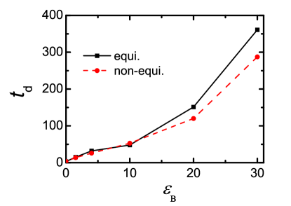
To test to what extent attractive forces can bind solute particles to the colloid, we probe , the number of particles that remain bound to the colloid (i.e. ) for at leats time-steps. decays exponentially with time (see SI). The rate of decay is a measure for the characteristic time during which a fluid particle is bound to the colloid. The dependence of on is shown in Fig. 4. As expected, increases with . We also note that decreases with increasing flow rate: the difference woith the equilibrium case is most pronounced for larger values of .
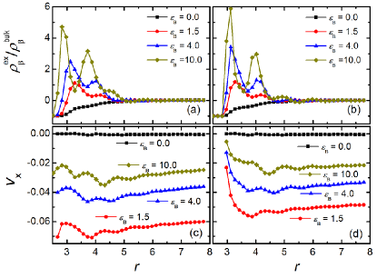
Figs. 5(a-b) compare the radial distribution of the reduced excess density of the solutes. For both slip and non-slip boundaries, when is increased from to , significant excess of solutes near the colloid is observed. When is further increased, the solutes close to the colloid are effectively trapped and form a rigid shell at around that does not contribute to diffusio-phoresis. The peak is higher and sharper for non-slip boundaries. Fig. 5(c-d) presents the radial profile of fluid velocity with slip and non-slip boundaries. As expected, for the magnitude of is decreasing due to the formation of the shell-region, and generally at the same the magnitude of is smaller for non-slip boundaries, particularly close to the colloid.
3.2 Anisotropic interaction
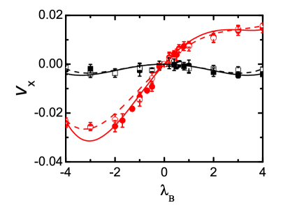
To distinguish between different symmetry classes of the anisotropic solute-colloid interactions, we assume that their angular dependence is proportional to Legendre polynomials (5). We note that the case is unique in the sense that it is the only anisotropic term for which a linear relation between gradient and flow is possible. For other values of , the flow vanishes in the limit of weak attraction and the phoretic flow velocity should depend at least quadratically on the strength of the colloid-solute attraction. This difference in behavior can be understood by noting that both and are polar vectors that transform as irreducible tensors of rank one. In the linear regime (i.e. the regime where depends linearly on ), the variation of with is given by a symmetric matrix. Such a matrix has two parts: the trace, which transforms as a scalar (=0), and the traceless symmetric part that transforms as second-rank irreducible tensor (=2). For isotropic particles, only the part contributes. However, if the interaction potential is anisotropic, then the part (i.e. the part of the interaction that transforms as ), can also contribute. However, all other angular dependence of the potential ( etc) do not contribute to linear order. Note, however, that when the interaction becomes stronger, other Legendre components of the potential may contribute to the phoretic flow, because the excess density depends exponentially on the potential. This means that the excess density then no longer has the same symmetry as the anisotropic potential. In that case, the positive and negative contributions to the excess solute density do no longer cancel, and hence there may still be a flow for, say, at larger values of . We have considered anisotropic interactions of first () and second () order and evaluated the phoretic flow velocity as a function of the magnitude .
The results are presented in Fig. 6 for slip (solid curves) and non-slip (dashed curves) boundary conditions. As expected, at small , the flow velocity depends linearly on the interaction strength for , but quadratically for . The difference between slip and non-slip boundary conditions is barely significant. We fit the simulated data with polynomials:
| (8) |
Powers up to fourth order () need to be considered to obtain a good fit to the data. Based on the above symmetry arguments, we require that for . Table 2 summarizes the fit coefficients for the four cases considered: and for slip and non-slip boundaries.
| l=1 | ||||
|---|---|---|---|---|
| slip | 0 | 0 | ||
| non-slip | 0 | 0 | ||
| l=2 | ||||
| slip | ||||
| non-slip |
4 Conclusions
The main findings of the present work are that, although in general the strength of diffusio-phoresis increases with the excess density of adsorbed solute, the diffusio-phoretic motion is suppressed if the binding between colloid and solute is very strong. In the limit of strong binding, the adsorbed layer becomes immobile and plays no role in phoresis. However, the phoretic velocity remains finite, even for very strong adsorption, presumably because of the structuring of the fluid around the strongly adsorbed layer. In addition, we investigated the effect on phoresis of angle-dependent interactions. In analogy with what is found for the electrophoresis of colloids with a thin double layer, we find that the diffusion phoretic effect changes qualitatively as the symmetry of the anisotropic interaction is changed. These findings demonstrate that the strength of diffusio-phoresis of particles with a patchy interaction (e.g. proteins) depends not just on the strength of the patchy interaction, but on the precise distribution of the patches over the surface of the particle.
Our simulations suggest that although diffusio-phoresis may in principle be used to induce selective transport of bio-macromolecules in a concentration gradient of selectively binding solutes, the non-monotonic dependence of the transport velocity on the binding strength limits the use of this approach, in the sense that there is no point in making the interaction of the bio-molecules with the solute very strong. It may then be more useful to selectively adsorb functionalized, charged solutes on the bio-molecules to make them more susceptible to electro-phoresis. Our simulations suggest that anisotropic interactions may enhance (or decrease) the diffusio-phoretic mobility of an otherwise spherical particle. However, as only the component of the anisotropic interaction contributes appreciably, the isotropic interaction will dominate the diffusio-phoresis of particles that have a large number of interaction “patches”.
Acknowledgements
This work was partially funded by the National Key Research and Development Program of China (grant 2016YFA0501601), by the EU Horizon 2020 program through 766972-FET-OPEN-NANOPHLOW, by K. C. Wong Educational Foundation, and by the National Natural Science Foundations of China under grants 11602279 and 11874398.
Notes and references
- Eijkel and van den Berg 2010 J. C. Eijkel and A. van den Berg, Chem Soc Rev, 2010, 39, 957–73.
- Anderson and Prieve 2006 J. L. Anderson and D. C. Prieve, Separation and Purification Methods, 2006, 13, 67–103.
- Annunziata et al. 2012 O. Annunziata, D. Buzatu and J. G. Albright, J Phys Chem B, 2012, 116, 12694–705.
- Ault et al. 2017 J. T. Ault, P. B. Warren, S. Shin and H. A. Stone, Soft Matter, 2017, 13, 9015–9023.
- Deseigne et al. 2014 J. Deseigne, C. Cottin-Bizonne, A. D. Stroock, L. Bocquet and C. Ybert, Soft Matter, 2014, 10, 4795–9.
- Khair 2013 A. S. Khair, Journal of Fluid Mechanics, 2013, 731, 64–94.
- Palacci et al. 2010 J. Palacci, B. Abecassis, C. Cottin-Bizonne, C. Ybert and L. Bocquet, Phys Rev Lett, 2010, 104, 138302.
- Paustian et al. 2015 J. S. Paustian, C. D. Angulo, R. Nery-Azevedo, N. Shi, A. I. Abdel-Fattah and T. M. Squires, Langmuir, 2015, 31, 4402–10.
- Prieve et al. 2019 D. C. Prieve, S. M. Malone, A. S. Khair, R. F. Stout and M. Y. Kanj, Proc Natl Acad Sci U S A, 2019, 116, 18257–18262.
- Sear and Warren 2017 R. P. Sear and P. B. Warren, Phys Rev E, 2017, 96, 062602.
- Shi et al. 2016 N. Shi, R. Nery-Azevedo, A. I. Abdel-Fattah and T. M. Squires, Phys Rev Lett, 2016, 117, 258001.
- Shin et al. 2017 S. Shin, J. T. Ault, P. B. Warren and H. A. Stone, Physical Review X, 2017, 7, year.
- Velegol et al. 2016 D. Velegol, A. Garg, R. Guha, A. Kar and M. Kumar, Soft Matter, 2016, 12, 4686–703.
- Yang et al. 2014 M. Yang, A. Wysocki and M. Ripoll, Soft Matter, 2014, 10, 6208–6218.
- Wurger 2010 A. Wurger, Reports on Progress in Physics, 2010, 73, 126601.
- Braibanti et al. 2008 M. Braibanti, D. Vigolo and R. Piazza, Phys Rev Lett, 2008, 100, 108303.
- Burelbach et al. 2017 J. Burelbach, D. Frenkel, I. Pagonabarraga and E. Eiser, The European Physical Journal E, 2017, 41, 7.
- Burelbach et al. 2017 J. Burelbach, M. Zupkauskas, R. Lamboll, Y. Lan and E. Eiser, J Chem Phys, 2017, 147, 094906.
- Fu et al. 2017 L. Fu, S. Merabia and L. Joly, Phys Rev Lett, 2017, 119, 214501.
- Maeda et al. 2011 Y. T. Maeda, A. Buguin and A. Libchaber, Phys Rev Lett, 2011, 107, 038301.
- Piazza 2008 R. Piazza, Soft Matter, 2008, 4, 1740.
- Piazza and Parola 2008 R. Piazza and A. Parola, Journal of Physics: Condensed Matter, 2008, 20, 153102.
- Tsuji et al. 2017 T. Tsuji, K. Kozai, H. Ishino and S. Kawano, Micro and Nano Letters, 2017, 12, 520–525.
- Vigolo et al. 2010 D. Vigolo, R. Rusconi, H. A. Stone and R. Piazza, Soft Matter, 2010, 6, 3489.
- Vigolo et al. 2017 D. Vigolo, J. Zhao, S. Handschin, X. Cao, A. J. deMello and R. Mezzenga, Sci Rep, 2017, 7, 1211.
- Wienken et al. 2010 C. J. Wienken, P. Baaske, U. Rothbauer, D. Braun and S. Duhr, Nat Commun, 2010, 1, 100.
- Wolff et al. 2016 M. Wolff, J. J. Mittag, T. W. Herling, E. D. Genst, C. M. Dobson, T. P. Knowles, D. Braun and A. K. Buell, Sci Rep, 2016, 6, 22829.
- Molotilin et al. 2016 T. Y. Molotilin, V. Lobaskin and O. I. Vinogradova, J Chem Phys, 2016, 145, 244704.
- Semenov et al. 2013 I. Semenov, S. Raafatnia, M. Sega, V. Lobaskin, C. Holm and F. Kremer, Phys Rev E Stat Nonlin Soft Matter Phys, 2013, 87, 022302.
- Stout and Khair 2017 R. F. Stout and A. S. Khair, Phys. Rev. Fluids, 2017, 2, 014201.
- Tanaka and Grosberg 2002 M. Tanaka and A. Y. Grosberg, Eur Phys J E Soft Matter, 2002, 7, 371–9.
- Tanaka 2003 M. Tanaka, Phys Rev E Stat Nonlin Soft Matter Phys, 2003, 68, 061501.
- Anderson 1981 J. L. Anderson, Journal of Colloid and Interface Science, 1981, 82, 248–250.
- Yang et al. 2017 M. Yang, R. Liu, F. Ye and K. Chen, Soft Matter, 2017, 13, 647–657.
- Chen et al. 2017 T. Chen, C. Xu and Z. Ren, Journal of Industrial Management Optimization, 2017, 13, 1–19.
- Huang et al. 2016 M.-J. Huang, J. Schofield and R. Kapral, Soft Matter, 2016, 12, 5581–5589.
- Liu et al. 2018 Y. Liu, R. Ganti and D. Frenkel, Journal of Physics: Condensed Matter, 2018, 30, 205002.
- Sharifi-Mood et al. 2013 N. Sharifi-Mood, J. Koplik and C. Maldarelli, Phys Rev Lett, 2013, 111, 184501.
- Abecassis et al. 2008 B. Abecassis, C. Cottin-Bizonne, C. Ybert, A. Ajdari and L. Bocquet, Nat Mater, 2008, 7, 785–9.
- Banerjee et al. 2016 A. Banerjee, I. Williams, R. N. Azevedo, M. E. Helgeson and T. M. Squires, Proceedings of the National Academy of Sciences, 2016, 113, 8612–8617.
- Saar et al. 2017 K. L. Saar, Y. Zhang, T. Muller, C. P. Kumar, S. Devenish, A. Lynn, U. Lapinska, X. Yang, S. Linse and T. P. J. Knowles, Lab Chip, 2017, 18, 162–170.
- Yang and Ripoll 2016 M. Yang and M. Ripoll, Soft Matter, 2016, 12, 8564–8573.
- Liu et al. 2017 Y. Liu, R. Ganti, H. G. Burton, X. Zhang, W. Wang and D. Frenkel, Physical Review Letters, 2017, 119, 224502.
- Yoshida et al. 2017 H. Yoshida, S. Marbach and L. Bocquet, The Journal of Chemical Physics, 2017, 146, 194702.
- Ganti et al. 2017 R. Ganti, Y. Liu and D. Frenkel, Phys Rev Lett, 2017, 119, 038002.
- Wang et al. 2019 X. Wang, S. Ramírez-Hinestrosa, J. Dobnikar and D. Frenkel, The Lennard-Jones potential: when (not) to use it, 2019.
- Ramírez-Hinestrosa et al. 2019 S. Ramírez-Hinestrosa, H. Yoshida, L. Bocquet and D. Frenkel, Numerical analysis of polymer diffusiophoresis by means of the molecular dynamics, 2019.
- Bocquet and Barrat 1994 L. Bocquet and J. Barrat, Phys. Rev. E, 1994, 49, 3079–3092.