A Multi-Vector Interface Quasi-Newton Method with Linear Complexity for Partitioned Fluid-Structure Interaction
Abstract
In recent years, interface quasi-Newton methods have gained growing attention in the fluid-structure interaction community by significantly improving partitioned solution schemes: They not only help to control the inherent added-mass instability, but also prove to substantially speed up the coupling’s convergence. In this work, we present a novel variant: The key idea is to build on the multi-vector Jacobian update scheme first presented by Bogaers et al. [1] and avoid any explicit representation of the (inverse) Jacobian approximation, since it slows down the solution for large systems. Instead, all terms involving a quadratic complexity have been systematically eliminated. The result is a new multi-vector interface quasi-Newton variant whose computational cost scales linearly with the problem size.
keywords:
Fluid-Structure Interaction , Interface Quasi-Newton Methods , Partitioned Algorithm1 Introduction
Partitioned solution schemes for fluid-structure interaction (FSI) are widely used in modern computational engineering science, as they offer great flexibility and modularity concerning the two solvers employed for the fluid and the structure. Treated as black boxes, the solvers are coupled only via the exchange of interface data. The major downside of partitioned schemes, however, is an inherent instability caused by the so-called added-mass effect [2, 3]. Depending on the application, its influence might be severe enough to impede a numerical solution – if no counter-measures are taken.
The simplest way to retain stability is a relaxation of the exchanged coupling data. The relaxation factor might either be constant or updated dynamically via Aitken’s method [4, 5]. Unfortunately, the high price to be paid in terms of the coupling’s convergence speed often renders this approach infeasible.
As opposed to this, interface quasi-Newton (IQN) methods have proven capable of both stabilizing and accelerating partitioned solution schemes [6, 7, 8]. Identifying the converged solution as a fixed point, their basic idea is to speed up the coupling iteration using Newton’s method. Since the required (inverse) Jacobian is typically not accessible, interface quasi-Newton approaches settle for approximating it instead.
Early work in the field has been done by Gerbeau et al. [9] as well as van Brummelen et al. [10]. A breakthrough, however, was the interface quasi-Newton inverse least-squares (IQN-ILS) method by Degroote et al. [11]: On the one hand, it directly solves for the inverse Jacobian required in the Newton linearization; on the other hand, the IQN-ILS variant introduces the least-squares approximation based on input-output data pairs that is still common today.
Research of the last decade has shown that a reutilization of data pairs from previous time steps is extremely advantageous. Unfortunately, an explicit incorporation in the IQN-ILS method suffers from numerical difficulties such as rank deficiency; moreover, good choices for the number of incorporated time steps are in general problem-dependent [12, 13]. However, the works by Degroote and Vierendeels [14] as well as Haltermann et al. [15] have shown that filtering out linearly dependent data pairs is an effective way of alleviating these issues.
As an alternative, Bogaers et al. [1] and Lindner et al. [13] formulated a very beneficial implicit reutilization of past information, yielding the interface quasi-Newton inverse multi-vector Jacobian (IQN-IMVJ) method. Its only real drawback is the required explicit representation of the approximated inverse Jacobian: Since the related cost is increasing quadratically with the number of degrees of freedom at the FSI boundary, this explicit form seriously slows down the numerical simulation for larger problem scales.
In this work, we present an enhancement of the IQN-IMVJ concept tackling exactly this shortcoming:
Retaining the effective implicit reutilization of past data,
the new interface quasi-Newton implicit multi-vector least-squares (IQN-IMVLS) method
completely avoids any explicit Jacobian or quadratic dependency
on the interface resolution.
While the advantages of the multi-vector approach are preserved,
the resulting linear complexity ensures the negligibility of computational cost
even for large problem scales.
This paper is structured as follows: Section 2 presents the governing equations of the considered FSI problems, before Section 3 briefly covers the numerical methods applied to solve them. In Section 4, the IQN-ILS and the IQN-IMVJ approach are discussed in detail, before the IQN-IMVLS method is derived. The efficiency of the new approach is validated in Section 5 based on numerical test cases.
2 Governing Equations
In general, fluid-structure interaction considers a fluid domain and a structure , that are connected via a shared boundary , the FSI interface. The subscript refers to the time level, while denotes the number of spatial dimensions. This section introduces the models and equations employed for the two subproblems along with the boundary conditions interlinking their solutions at the shared interface.
2.1 Fluid Flow
The velocity and the pressure of the fluid are governed by the unsteady Navier-Stokes equations for an incompressible fluid, reading
| (1a) | |||||
| (1b) | |||||
Therein, is the constant fluid density, while denotes the resultant of all external body forces per unit mass of fluid. For a Newtonian fluid with the dynamic viscosity , the Cauchy stress tensor is modeled by Stokes law as
| (2) |
The problem is closed by defining not only a divergence-free initial velocity field , but also a prescribed velocity on the Dirichlet boundary and prescribed tractions on the Neumann boundary with its outer normal :
| (3a) | |||||
| (3b) | |||||
| (3c) | |||||
2.2 Structural Deformation
The response of the structure to external loads is expressed via the displacement field , which is governed by the equation of motion, stating a dynamic balance of inner and outer stresses:
| (4) |
In this relation, denotes the material density and the resultant of all body forces per unit volume, whereas represents the Cauchy stress tensor.
As constitutive relation, the St. Venant-Kirchhoff material model is used: It relates the 2nd Piola-Kirchhoff stresses to the Green-Lagrange strains via a linear stress-strain law, reading
| (5) |
Therein, denotes the deformation gradient, while and are the Lamé constants. As the Green-Lagrange strain definition forms a nonlinear kinematic relation, the structural model is geometrically nonlinear. Hence, it is capable of representing large displacements and rotations, but only small strains [16, 17].
Collecting all this information, the equation of motion can be expressed in the (undeformed) reference configuration in a total Lagrangian fashion:
| (6) |
Again, the problem is closed by defining an initial displacement , which is typically zero, and a set of boundary conditions on two complementary subsets of : Prescribing the displacement on the Dirichlet part and the tractions on the Neumann part , with the outer normal in the reference state , the conditions read
| (7a) | |||||
| (7b) | |||||
| (7c) | |||||
2.3 Coupling Conditions at the Interface
The essence of fluid-structure interaction is that the two subproblems cannot be solved independently, since their solution fields are interlinked via the so-called coupling conditions arising at the shared interface :
-
1.
The kinematic coupling condition requires the continuity of displacements and , velocities and , and accelerations and across the FSI boundary [18]:
(8a) (8b) (8c) -
2.
In agreement with Newton’s third law, the dynamic coupling condition,
(9) enforces the equality of stresses at the interface. Therein, and denote the associated normal vectors [19].
In the continuous problem formulation, satisfying both these coupling conditions for every time ensures the conservation of mass, momentum, and energy over the FSI boundary [20].
3 Numerical Methods
3.1 Flow Solution
The Navier-Stokes equations formulated in Section 2.1 are discretized in this work using P1P1 finite elements, i.e., linear interpolations for both velocity and pressure. Numerical instabilities, caused by P1P1 elements violating the LBB condition, are overcome using a Galerkin/Least-Squares (GLS) stabilization [21, 22].
Contrary to the usual practice, both space and time are discretized by finite elements. More precisely, we employ the deforming-spatial-domain/stabilized-space-time (DSD/SST) approach introduced by Tezduyar and Behr [23, 24]. By formulating the variational form over the space-time domain, this approach inherently accounts for an evolving spatial domain. While the finite-element interpolation functions are continuous in space, the linear discontinuous Galerkin ansatz in time allows to solve one space-time slab after another.
3.2 Structural Solution
The structural subproblem is discretized in space by isogeometric analysis [27], while the time integration is performed using the generalized- scheme [28, 29].
3.2.1 Isogeometric Analysis (IGA)
Introduced by Hughes et al. [30] in 2005, isogeometric analysis is a finite-element variant aimed at achieving geometrical accuracy and a closer linkage between CAD and numerical analysis . The essential idea is to express the solution space via the same basis functions as used for the geometry description. Since CAD systems are commonly based on non-uniform rational B-Splines (NURBS), we choose a NURBS ansatz for the unknown displacement field. Mathematically, a NURBS is a linear combination of its control points and the rational basis functions , defined in the parameter space , with the spline dimension [31]. A NURBS surface hence has the form
| (10) |
3.2.2 Shell Theory
Shell structures are thin-walled structures capable of providing lightweight, cost-efficient and yet stable constructions for numerous engineering applications [32]. Mathematical shell models exploit the small thickness by reducing the structure from a volumetric description to the midsurface plus an interpolation over the thickness . Combining isogeometric analysis with Reissner-Mindlin shell theory, a NURBS midsurface and a linear interpolation are chosen; any position in the structural domain is hence expressed as
| (11) |
The parametric coordinate changes along the thickness direction, defined by the director vector . Consequently, the unknown displacement field is a combination of the midsurface displacement and a second term accounting for changes of the director vector :
| (12) |
3.3 Coupling Approach
This work pursues a partitioned FSI coupling approach: Two distinct solvers are employed for the fluid and the structure; they are connected via a coupling module, which handles the exchange of interface data in accordance to the coupling conditions. While the strengths of this approach are its great flexibility and modularity regarding the single-field solvers, these advantages come at the price of additional considerations to be made in terms of data exchange:
-
1.
In general, the meshes – or even the discretization techniques – do not match at the FSI boundary. Hence, a conservative projection is required to transfer relevant data between the two solvers. In this work, we employ a spline-based variant of the finite interpolation elements (FIE) method; a detailed description can be found in Hosters et al. [36]. For the sake of observability, however, any effects of this spatial coupling are neglected in the following, since they do not interfere with the presented methods.
- 2.
3.3.1 Dirichlet-Neumann Coupling Scheme
Nowadays, the de facto standard among strong coupling approaches for FSI problems is the Dirichlet-Neumann coupling scheme illustrated in Figure 1:
The first coupling iteration () of a new time step starts with the fluid solver: Based on the interface deformation of time level (or an extrapolated one), it computes a new flow field. In compliance with the dynamic coupling condition, the resulting fluid stresses acting on are passed as a Neumann condition to the structural solver, which determines the corresponding interface deformation . If it matches (within a certain accuracy) the previous deformation , i.e., , the coupled system has converged and we can go on to the next time step. Otherwise, the interface deformation is passed back to the flow solver as a Dirichlet condition, following kinematic continuity, and the next coupling iteration is started.
From a mathematical point of view, the Dirichlet-Neumann coupling scheme can be interpreted as a fixed-point iteration of the deformation at the interface [4, 13]; the fixed-point operator corresponds to the two subsequent solver calls, i.e., to running one coupling iteration :
| (13) |
Finding the converged solution of the next time level is hence equivalent to finding a fixed point of the interface deformation. Defining the fixed-point residual and its inverse as
| (14a) | |||||||
| (14b) | |||||||
with , the convergence criteria can analogously be expressed as a root of the residual, i.e., .
Note that although it is much less common, the fixed-point ansatz and the convergence criteria could analogously be formulated based on the fluid loads at the FSI interface.
3.3.2 Added-Mass Instability
Unfortunately, partitioned algorithms for fluid-structure interaction involving incompressible fluids exhibit an inherent instability, which may be severe, depending on the simulated problem. This so-called (artificial) added-mass effect originates from the CFD forces inevitably being determined based on a defective structural deformation during the iterative procedure. As a consequence, they differ from the correct loads of the next time level. This deviation potentially acts like an additional fluid mass on the structural degrees of freedom. More precisely, due to the kinematic continuity an overestimated structural deformation entails an exaggerated fluid acceleration – and hence excessive inertia stress terms. In many cases the effect is amplified throughout the coupling iterations, causing a divergence of the coupled problem. A major influencing factor are high density ratios between the fluid and the structure, , but dependencies on the viscous terms and the temporal discretization are observed, too. We recommend the works by Förster [2], Förster et al. [3], and Causin et al. [37] for more details on the added-mass effect. Moreover, van Brummelen et al. [38] investigate similar difficulties for compressible flows.
3.3.3 Stabilizing and Accelerating the Coupling Scheme
One way to deal with the added-mass instabilities is to adjust the computed interface deformation by an update step before passing it back to the flow solver. Depending on the chosen update technique, both the stability and efficiency of the coupling scheme can be improved.
The simplest way to increase stability is a constant under-relaxation of the interface deformation:
| (15) |
with . Effectively, it yields an interpolation between the current and the previous interface displacements and . As the factor must be chosen small enough to avoid the coupling’s divergence for any time step, unfortunately this approach often comes at a very high price in terms of efficiency [7]. Aitken’s dynamic relaxation [4, 5] tackles this issue by dynamically adapting the relaxation factor in Equation (15) for each coupling iteration by
| (16) |
i.e., based on the two most recent fixed-point residuals and .
Despite its rather simple implementation,
in many cases
Aitken’s relaxation provides significant speed-ups
without perturbing the stability of the relaxation.
Still, the performance of the coupling scheme can be pushed further by
more sophisticated approaches like
interface quasi-Newton (IQN) methods.
Remark 1: In the following, we will express the interface deformation as the structural solution at the FSI interface. While its representation via the boundary displacement of the fluid mesh is likewise possible, the typically finer interface resolution would result in higher numerical cost for the discussed update techniques.
4 Interface Quasi-Newton Methods
4.1 Interface Quasi-Newton Inverse Least-Squares (IQN-ILS) Method
In a partitioned solution procedure for fluid-structure interaction, the single-field solvers are typically the most expensive part, rendering all further costs, e.g., for data exchange, negligible in comparison [1, 39].
Since the converged time step solution has been identified as a root of the fixed-point residual or its inverse form defined in Equation (14), increasing the efficiency essentially comes down to reducing the number of coupling iterations required to find such a root. Consequently, employing Newton’s method as an update step of the interface deformation would be a promising approach to speed up convergence, yielding [11, 13]
| (17) |
Unfortunately, an evaluation of the required inverse Jacobian in general is not accessible, as it would involve the derivatives of both the fluid and the structural solver. The idea of interface quasi-Newton methods is to circumvent this issue by approximating the (inverse) Jacobian rather than evaluating it exactly. Using a Taylor expansion of , we can approximate via
| (18) |
based on an input-output data pair. Such a pair is formed by some change in the interface deformation and the corresponding change of the fixed-point residual . Therein, denotes the number of structural degrees of freedom at the FSI interface. Essentially, this idea is an -dimensional version of approximating a derivative with the slope of a secant. To avoid additional solver calls, the required data pairs are formed from the intermediate results and of the coupling iterations already performed for the current time step. More precisely, they are stored in the input matrix and the output matrix [12]:
| (19a) | ||||||||||
| (19b) | ||||||||||
With the collected data, an approximation of the inverse Jacobian can be formulated via
| (20) |
Since the number of data pairs stored in and typically is much smaller than the number of structural degrees of freedom at the FSI interface, i.e., , the linear system of equations (20) is underdetermined. The existence of a unique solution is ensured by demanding the minimization of the Frobenius norm [13]:
| (21) |
Together, equations (20) and (21) form a constrained optimization problem, which leads to an explicit form of the inverse Jacobian approximation [12, 13]:
| (22) |
Inserting this inverse Jacobian approximation into the Newton update formula in Equation (17) yields a quasi-Newton update scheme for the interface deformation,
| (23) |
Defining the vector exploits that the inverse Jacobian is not needed explicitly here, but only its product with the residual vector. An efficient way of computing is to solve the least-squares problem [11, 12]
| (24) |
e.g., using a QR decomposition via Householder reflections. In the first coupling iteration, a relaxation step is used, as no data pairs are available yet.
The approach presented so far is referred to as interface quasi-Newton inverse least-squares (IQN-ILS) method [11]; it can be interpreted as the basis of the other IQN variants discussed in this work.
4.2 Benefit from Previous Time Steps
So far, the inverse Jacobian of the residual operator is approximated only based on information gathered in the coupling iterations of the current time step. In principle, however, the efficiency of IQN methods can be significantly increased by incorporating data from previous time steps as well. The most straightforward way to do so is to explicitly include the data pairs of past time steps in the input and output matrices and [11].
Unfortunately, apart from increasing costs for handling big data sets, a growing number of data pairs stored in these matrices entails two major problems [1, 13, 40]: (1) The matrix might be very close to rank-deficient due to (almost) linear dependent columns; related to that, the condition number of the least-squares problem quickly increases; (2) information gathered in different time steps might be contradictory. Together, these drawbacks carry the risk of preventing the system from being numerically solvable at all.
An obvious remedy is to incorporate only the data of the most recent time steps. While this approach is in fact capable of yielding a superior convergence speed, its major shortcomings are the risk of rank deficiency and in a good choice for the parameter being problem-dependent [1, 12]. One way to mitigate these drawbacks is by employing a filtering technique [14, 15].
4.3 Interface Quasi-Newton Inverse Multi-Vector Jacobian Method
An alternative way of reusing data from previous time steps was introduced by Bogaers et al. [1] and developed further by Lindner et al. [13]: The interface quasi-Newton inverse multi-vector Jacobian (IQN-IMVJ) method combines the IQN approach with the idea of Broyden’s method: In a Newton iteration, one might expect the Jacobians evaluated in subsequent iterations to be similar in some sense. Therefore, Broyden’s method limits the typically costly Jacobian evaluation to the first iteration only; after that, the new Jacobian is instead approximated by a rank-one update of the previous one. For the interface quasi-Newton framework, this concept is adopted by formulating the current inverse Jacobian approximation as an update of the one determined in the previous time step :
| (25) |
where denotes the update increment. Introducing this concept changes the constrained optimization problem discussed in Section 4.1 to
| (26) |
This system allows for a quite descriptive interpretation: Fitting Broyden’s idea, the difference between the inverse Jacobians of the current and the previous time step is minimized, rather than the norm of the approximation itself.
Again, the result is an explicit approximation of the current inverse Jacobian [13]:
| (27) |
In contrast to the IQN-ILS approach, the IQN-IMVJ method explicitly updates the Jacobian in every coupling iteration via Equation (27). Therein, the matrix is determined by solving the least-squares problem
| (28) |
for each column with the -th unit vector , again using a Householder QR decomposition. After has been updated, the quasi-Newton step is performed:
| (29) |
Since the inverse Jacobian is initialized to zero, i.e., , the first time step is equivalent to the IQN-ILS method.
Note that the matrices and only contain data collected in the current time step; because, rather than explicitly including data pairs collected in previous time steps, the IQN-IMVJ approach incorporates them implicitly in form of the previous Jacobian approximation . This implicit reutilization of past information entails some significant advantages [1, 13]: (1) Since the matrices and are not affected, neither is the condition number of the least-squares problem; (2) it renders any tuning of (strongly) problem-dependent parameters obsolete; (3) since past information is matched in a minimum norm sense only, it is automatically less emphasized than that of the current time step. This avoids the risk of relying on outdated or contradicting data.
These benefits come at the price of an explicit representation of the inverse Jacobian approximation, that is often very expensive to store and handle, as the entailed complexity is growing quadratically with the problem scale.
4.4 Interface Quasi-Newton Implicit Multi-Vector Least-Squares Method
In this paper, we introduce an enhancement of the IQN-IMVJ approach
tackling its main issue, i.e., the high cost
related to the explicit Jacobian approximation.
By successively replacing the expensive parts,
this section derives the new interface quasi-Newton implicit multi-vector least-squares (IQN-IMVLS) method.
As a first step, the explicit use of the current inverse Jacobian approximation is eliminated: By inserting the Jacobian update (27) into the quasi-Newton step, the vector can be identified in analogy to the IQN-ILS approach, changing the update formula to
| (30) |
By reducing the least-squares problem back to Equation (24), this drastically reduces the computational cost. The past inverse Jacobian , however, is still explicitly required: Once a time step has converged, it is updated to the next time level by Equation (27); the associated cost is quadratic in . Beyond that, is involved in the quasi-Newton formula in Equation (30). In particular, it is needed for the potentially very costly matrix product in , which has a complexity of . As mentioned before, however, the matrices and are successively built up only by appending new columns. Taking this into account, we can reformulate
| (31) |
As a consequence, restoring the terms and from the previous iteration in fact allows to reduce the number of matrix-vector products with the inverse Jacobian to one per coupling iteration, that is .
This Jacobian-vector product remains the only operation in Equation (30) involving an complexity. For an increasing number of structural degrees of freedom at the interface , this term’s cost therefore may become dominant and slow down the overall procedure (see Remark 4.4).
In order to tackle this issue, we introduce an alternative purely implicit formula for evaluating without any explicit previous Jacobian . Note that the explicit Jacobian update will become obsolete as a direct consequence. Unraveling the recursion in Equation (27), the update of the inverse Jacobian can be reformulated to
| (32) |
see A for the proof. Therein, the upper index of the matrices , , and refers to the time step they were determined in. Considering the initial Jacobian approximation, , this expression simplifies to
| (33) |
While being mathematically equivalent, this formulation entails two main advantages: First, the matrix-vector product can be determined in an implicit manner via
| (34) |
without an complexity, and hence potentially cheaper. However, the cost for evaluating the expression in Equation (34) obviously increases with the number of processed time steps. This issue is addressed using the second advantage: While data from past time steps is still incorporated in an implicit manner, with all the associated advantages discussed in Section 4.3, the new formulation explicitly identifies the contribution of each time step, in the form of the matrices , , and . As a consequence, this update technique allows to incorporate only the most recent time steps for the previous Jacobian approximation as a way of limiting the cost of the matrix-vector product, which then reads
| (35) |
In fact, by taking advantage of the repetition of terms in the product (see B), this expression can be evaluated in , where denotes the average number of coupling iterations per time step. This step can be justified by the fact that a certain time step’s contribution to the previous Jacobian approximation is gradually becoming less and less important the further the simulation progresses.
At a first glance, one might argue that the parameter reintroduces exactly the problems the multi-vector approach was designed to avoid in the first place, i.e., the dependency of the IQN-ILS method on the number of reused time steps. However, this issue arose from the explicit incorporation of past data, e.g., due to high condition numbers and linear-dependent columns in . Since the IQN-IMVLS approach reuses data in an implicit manner, it does not suffer from these drawbacks. Instead, the method’s quality in general benefits from increasing the number of past time steps taken into account, as the limit of reusing all steps is analytically equivalent to the explicit Jacobian multiplication.
For this variant, the matrix still has to be determined and stored once after each time step. Since the complexity of computing it via the least-squares problems (28) is for the Householder QR approach, i.e., growing quadratically with , we use a matrix inversion of via a LU decomposition using partial pivoting with row interchanges instead [41]. While being slightly less robust to bad conditioning, the big advantage is that it requires operations and therefore scales linearly with the problem size.
Combining all this, the modified multi-vector update completely avoids any -terms that might slow down the IQN-IMVLS approach for large systems, where holds, see Table 4.4. A pseudo-code realization of the purely implicit IQN-IMVLS method is outlined in Algorithm 1.
| Increment step: | |||
| Operation | Expression | Explicit | Implicit |
| Least-squares problem | |||
| via Householder QR | |||
| Matrix-vector product b ^k = ^n ^J_-1 R_km^2m ¯k q | m | m | |
| Matrix-vector product B _k αm ¯km ¯k | |||
| Operation | Expression | Explicit | Implicit |
| Least-squares problem | – | ||
| via Householder QR | |||
| Matrix-matrix product B _k Z_km^2 ¯k | |||
| Determine and store | |||
| Operation | Expression | Explicit | Implicit |
| Matrix inversion via | – | ||
| LU decomposition | |||
| Matrix-matrix product -1 V_k^T | |||
In direct analogy to the computational complexity, the memory requirements, too, are no longer scaling quadratically but linearly with the problem size: Although the matrices as well as have to be stored for the most recent time steps, the required amount of storage is much smaller than for the explicit Jacobian as long as holds.
Of course, the effectiveness of the purely implicit IQN-IMVLS update strongly depends on this ratio of and , so that the explicit Jacobian approximation might still be the better option for small systems. However, the assumption is not very restrictive for common application scales.
| Initialization: | , , |
|---|---|
| First iteration: | |
| Form residual: |
| Under-relaxtion step: |
| Previous inverse Jacobian times residual (implicitly): | |
|---|---|
| IQN-update with Jacobian product: |
| Perform coupling iteration: | |
|---|---|
| Form residual: | |
| Append new column to input matrix: | |
| Append new column to output matrix: | |
| Previous inverse Jacobian times residual (implicitly): | |
| Build restoring terms from previous iteration: | |
| Solve least-squares problem: | |
| Implicit update step: |
| Determine via LU decomposition: | |
| Store for future time steps: | , , Store |
Remark 2: Aside from suggesting improvements similar to using an explicit past Jacobian within the IQN-IMVLS method, Scheufele and Mehl [12] also derived a multi-vector variant with linear complexity. Therein, the past inverse Jacobian is represented based on the matrices and from past time steps, i.e.,
| (36) |
While the idea to avoid the costly explicit Jacobian via a sum formulation is similar to the IQN-IMVLS method, there is one essential difference: Due to the recursive definition of the multi-vector Jacobian approximation, each matrix contains information from the first time steps. By implication, this means that the contribution of a time step is contained in all subsequent matrices , , , and so forth. As a consequence, it is impossible to drop old time steps from the approximation while keeping more recent ones, as the IQN-IMVLS method does.
Instead, Scheufele and Mehl divide the simulation into chunks of several time steps; after each of these chunks, the sum in equation (36) has to be reset. Since a plain erasure of old data at every restart dramatically impairs the efficiency of the multi-vector approach, focus is put on different restart options: In particular, they introduce the multi-vector Jacobian restart singular value decomposition (IQN-MVJ-RS-SVD) method, in which a truncated SVD accounts for the dropped data. It introduces two main parameters: While the influence of the chunk size is typically less marked, the method’s accuracy and efficiency strongly depends on the threshold for cutting off insignificant singular values. However, choices around were shown to be suitable for various test cases [12]. For an in-depth discussion of the method refer to Scheufele and Mehl [12, 42].
In contrast to this restart-based approach, the IQN-IMVLS method always considers the most recent time steps. In combination with its arguably simpler implementation, it therefore represents a straightforward way of achieving a linear complexity without any need for restart techniques.
Remark 3: In the beginning of a new time step, the input and output matrix of the IQN-IMVLS method rely on very few data pairs only. To improve the significance of the least-squares problem, it can be beneficial to include the information of the most recent time step explicitly in the matrices and – in addition to the implicit reutilization of past data. The effect of this option will be included in the discussion of the numerical test cases in Section 5.
Remark 4: The computational cost of the interface quasi-Newton approaches discussed in this work increases with the number of structural degrees of freedom at the FSI interface. To assess the significance of this cost in comparison to the solver calls, the complexity of the structural solution is therefore of particular interest. Nowadays, the structural subproblem is typically solved using some finite-element variant, such as isogeometric analysis. These procedures can be subdivided into two main tasks: (1) The assembly of the system matrices is done in an element-by-element manner and hence scales with the number of elements , i.e., . Moreover, each of the degrees of freedom causes nonzero entries in the sparse system matrix [43]. As this number primarily depends on the element type this yields . For common meshes, is a reasonable estimate [44]. (2) Usually, an iterative solver is employed for solving the resulting sparse linear system of equations. In the ideal case, the associated computational complexity is [45, 46]. Since increasing the number of unknowns typically brings along a moderately growing number of solver iterations , the total complexity of the structural subproblem is expected to be superlinear, but significantly lower than quadratic.
5 Numerical Results
5.1 Elastic Pressure Tube
The first test case considers an elastic cylindrical tube that is filled with an incompressible fluid, as depicted in Figure 2a. Caused by a short excitation in the beginning, a pressure pulse propagates through the pipe structure. While the configuration is inspired by similar test cases discussed, among others, by Degroote et al. [7] and Lindner et al. [13], the prescribed pressure pulse is increased by a factor of ten.
The tube has a length of , an inner radius of , and a wall thickness of . The elastic structure is characterized by the density , its Young’s modulus , and a Poisson ratio of ; the fluid’s density is and its dynamic viscosity . Based on the density ratio of , a strong added-mass instability is to be expected.
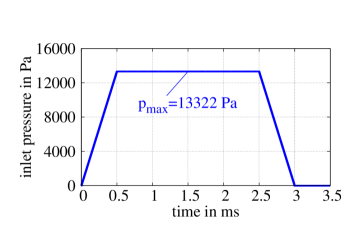
Both ends of the channel allow a free in- and outflow of the fluid. While a constant pressure of is prescribed on one end, the other one is excited by a short pressure pulse with a peak of in the beginning of the simulation, see Figure 2b. After that, its boundary pressure is held fixed at as well.
The fluid domain is discretized by tetrahedral elements with nodes per time level, i.e., a total of nodes due to the space-time formulation. The mesh is locally refined in the vicinity of the walls and near the prescribed pressure pulse. The elastic structure is clamped at both ends; it is represented by nonlinear isogeometric shell elements defined by a quadratic NURBS. This spline surface has control points and degrees of freedom. The simulation runs till in time steps of size . The convergence of the coupling scheme is detected by a combination of an absolute bound and a relative criterion for the norm of the fixed-point residual .
5.1.1 Results
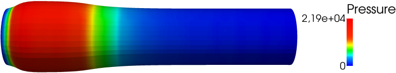
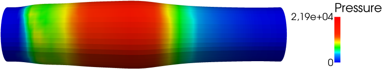
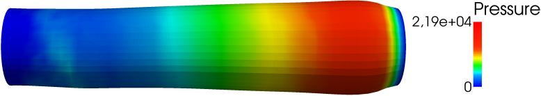
As stated above, the excitation causes a pressure pulse propagating through the elastic tube, which is depicted in Figure 4.4 for three sample time levels. The snapshots show that the moving pressure peak is accompanied by a large widening of the structure. While retaining its basic profile on its way through the pipe, the pulse clearly exhibits some diffusive flattening. Qualitatively, the numerical results agree with both physical expectations and the discussions of similar test cases in literature [1, 11, 13]. Note that this solution is independent (within the chosen convergence tolerance) from the update technique employed.
The focus of this test case is on the efficiency of different updating schemes. A comparison is provided in Table 2: Aside from the average number of coupling iterations per time step, it lists the relative speed-up in terms of coupling iterations and runtime with respect to a constant under-relaxation; lastly, the percentages of computation time spent for the interface quasi-Newton update are indicated.
| Method | Average Coupling | Relative Coupling | Relative | IQN-Time / |
|---|---|---|---|---|
| Iterations | Iterations | Runtime | Runtime | |
| Under-relaxation, | 100.39 | 100.00 % | 100.00 % | - |
| Aitken’s relaxation | 26.38 | 26.28 % | 26.31 % | - |
| IQN-ILS () | 14.96 | 14.90 % | 14.93 % | 0.087 % |
| IQN-ILS, | 8.91 | 8.88 % | 9.18 % | 0.122 % |
| IQN-ILS, | 8.06 | 8.03 % | 8.33 % | 0.426 % |
| IQN-ILS, | 8.66 | 8.63 % | 9.03 % | 1.042 % |
| IQN-ILS, | 9.76 | 9.72 % | 10.14 % | 2.890 % |
| IQN-IMVJ | 8.11 | 8.08 % | 9.53 % | 11.736 % |
| IQN-MVJ-RS-SVD, , | 8.09 | 8.06 % | 8.41 % | 0.370 % |
| IQN-IMVLS, explicit Jacobian | 8.14 | 8.10 % | 8.50 % | 1.263 % |
| IQN-IMVLS, | 8.54 | 8.50 % | 8.93 % | 0.070 % |
| IQN-IMVLS, | 8.28 | 8.24 % | 8.68 % | 0.078 % |
| IQN-IMVLS, | 7.95 | 7.92 % | 8.28 % | 0.089 % |
| IQN-IMVLS, | 8.05 | 8.02 % | 8.34 % | 0.113 % |
| IQN-IMVLS, | 8.05 | 8.02 % | 8.35 % | 0.120 % |
| IQN-IMVLS, , 1 explicit step | 7.76 | 7.73 % | 8.02 % | 0.253 % |
The first observation is that, although Aitken’s dynamic relaxation converges much faster than the constant under-relaxation, neither of them is really feasible for this test case, since they require about or coupling iterations per time step, respectively. The problem is the high added-mass instability, requiring very small relaxation factors; in this case, was found to be the highest value precluding divergence.
As opposed to this, all employed interface quasi-Newton variants entail a substantial increase in performance – both in terms of reducing the number of coupling iterations and the runtime. In particular, the incorporation of data from past time steps proves very beneficial. With this, using an IQN approach reduces the total runtime compared to a constant relaxation by up to ; perhaps even more remarkable is the decrease by about with respect to Aitken’s method.
The results for the IQN-ILS variant identify its dependency on the number of explicitly reused time steps : Away from the optimum of this test case, , including either too few or too many previous steps compromises the effectiveness; in fact, the coupling scheme was even diverging for values of higher than about . Note in this context that no filtering technique is applied within this work.
Against this backdrop, the implicit incorporation of past data via the previous inverse Jacobian deserves special notice: Despite not requiring any problem-dependent parameters, it enables the IQN-IMVJ variant to keep up with the optimum of the IQN-ILS approach in terms of coupling iterations. However, the actual runtime indicates its major drawback: While the computational cost of the IQN-ILS method barely exceeds of the total runtime for moderate choices of , handling the explicit Jacobian approximation raises the effort for the IQN-IMVJ method to ; hence, its cost is by no means negligible against the solver calls.
That is exactly what the IQN-IMVLS variant is designed to provide a remedy for. Since the analytic form of the quasi-Newton update stays untouched, the required coupling iterations of the IQN-IMVJ and the IQN-IMVLS approach with an explicit Jacobian show only an insignificant difference arising from numerical rounding. The IQN-IMVLS method, however, employs more advantageous numerical techniques and a beneficial storage of already determined quantities (as discussed in Section 4.4) to reduce the update’s computational cost. In particular, the number of operations involving an explicit Jacobian approximation is reduced. The results in Table 2 prove that these adjustments entail a significant speed-up of the multi-vector IQN approach – in this case by a factor of ten.
Moreover, the IQN-IMVLS method also provides a purely implicit version avoiding any explicit representation of the Jacobian approximation. This variant reintroduces the number of past time steps to be incorporated; in contrast to the explicit reutilization, however, this parameter is not very problem-dependent or critical, as high values of do not entail any numerical problems. Instead, the quality of the update scheme in general benefits from an increasing , as confirmed by Table 2: Although there seems to be a marginal optimum at around for this test case, the convergence speed afterwards aligns more and more with the one observed for including all past time steps (). In fact, it remains virtually unchanged for values higher than . In combination with the computational effort, which stays at around of the runtime even for including all previous steps, using the purely implicit update further improves the IQN-IMVLS method for this setting.
Without compromising effectiveness, the restart-based IQN-MVJ-RS-SVD method significantly reduces the cost of the multi-vector approach, too. Although being slightly more expensive than the new algorithm for this test case, the observed difference is small enough to be blurred by implementation details and parameter choices to some extent; in relation to the overall simulation time, both methods come at negligible cost.
When it comes to including the most recent time step explicitly in the IQN-IMVLS method as suggested in Remark 4.4, the last row in Table 2 confirms that this option does in fact slightly reduce the number of coupling iterations without being too expensive. The effect, however, is not very marked.
As indicated before, the main advantage of the purely implicit update, i.e., its linear complexity, becomes more distinct for larger problem scales. In general, the cost of the discussed interface quasi-Newton concept depends on the number of structural degrees of freedom at the FSI interface. As the elastic tube is modeled by shell elements, however, in this test case the FSI interface is equivalent to the whole structural domain. For shell analysis, a distinction between all structural degrees of freedom and those at the interface is redundant.
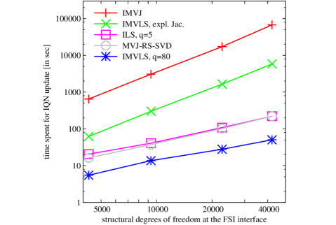
Therefore, Figure 4 plots the absolute time spent for the multi-vector IQN variants as well as the IQN-ILS method with over the number of structural degrees of freedom. To assess the complexity of the different methods, both axes are scaled logarithmically. The first observation is the exploding cost of the IQN-IMVJ method, caused by its extensive usage of the explicit Jacobian approximation. While the IQN-IMVLS method with an explicit inverse Jacobian again significantly reduces the numerical effort, it does not keep the cost from growing quadratically with the problem scale. In contrast, the purely implicit IQN-IMVLS version is not only much cheaper; the plot clearly points out its linear scaling with the interface resolution. Moreover, for this test setting it outperforms both the IQN-MVJ-RS-SVD and the IQN-ILS method, which also show a linear complexity.
| Method | Average Coupling | IQN / Structure |
|---|---|---|
| Iterations | in % | |
| Structural Degrees of Freedom (at the FSI Interface) | ||
| IQN-ILS, | 7.84 | 0.37 % |
| IQN-IMVJ | 8.01 | 27.36 % |
| IQN-MVJ-RS-SVD, , | 7.99 | 0.35 % |
| IQN-IMVLS, explicit Jacobian | 8.05 | 2.66 % |
| IQN-IMVLS, | 7.99 | 0.12 % |
| IQN-IMVLS, , 1 explicit step | 7.48 | 0.22 % |
| Structural Degrees of Freedom (at the FSI Interface) | ||
| IQN-ILS, | 8.20 | 0.33 % |
| IQN-IMVJ | 7.91 | 53.25 % |
| IQN-MVJ-RS-SVD, , | 8.09 | 0.32 % |
| IQN-IMVLS, explicit Jacobian | 7.99 | 5.08 % |
| IQN-IMVLS, | 7.86 | 0.09 % |
| IQN-IMVLS, , 1 explicit step | 7.79 | 0.19 % |
| Structural Degrees of Freedom (at the FSI Interface) | ||
| IQN-ILS, | 8.21 | 0.27 % |
| IQN-IMVJ | 7.99 | 83.58 % |
| IQN-MVJ-RS-SVD, , | 8.04 | 0.27 % |
| IQN-IMVLS, explicit Jacobian | 7.88 | 7.31 % |
| IQN-IMVLS, | 7.97 | 0.06 % |
| IQN-IMVLS, , 1 explicit step | 8.20 | 0.15 % |
While Figure 4 compares the efficiency of different quasi-Newton schemes, it does not allow any judgment on to which extent their computational cost is negligible compared to the solver calls. Therefore, Table 3 puts them into context: Taking into account that the fluid mesh does not have a direct influence on the IQN approach and that the structural domain is equivalent to the FSI interface due to the usage of shell elements, its last column relates the time spent for the quasi-Newton methods to that required for the structural solution; it considers three different levels of refinement of the structural discretization, i.e., , , and degrees of freedom. Moreover, Table 3 lists the average numbers of coupling iterations per time step, which stay close to for all tests conducted. Nevertheless, the investigated methods show vast differences regarding their computational cost.
Again, the most striking observation is the very high cost of the IQN-IMVJ method: For the three refinement levels, the runtime it accounts for ranges from to compared to the time required for the structural solution, and therefore seriously slows down the whole simulation. Moreover, this percentage is growing with the problem scale, indicating that the quadratic complexity causes the cost of the IQN-IMVJ approach to be increasing faster than that of solving the structural subproblem. As discussed before, the IQN-IMVLS method with an explicit Jacobian approximation significantly reduces the numerical effort, but not the method’s complexity; hence, its relative cost is still growing with the number of degrees of freedom, in this case from to . In contrast, the complexity of the purely implicit IQN-IMVLS version, the IQN-MVJ-RS-SVD method, and the IQN-ILS approach is linear. As a consequence, their portion on the total runtime is not only negligible for all the conducted simulations, but even decreasing with the structural refinement. In accordance to the discussion in Remark 4.4, these observations confirm that the complexity of solving the structural subproblem is between being linear and quadratic for this setting.
For the first and the second refinement levels, the explicit incorporation of the most recent time step in the least-squares problem of the IQN-IMVLS method again slightly accelerates the coupling. Unfortunately, the lower convergence speed for the finest level stands in the way of a general recommendation.
All in all, the purely implicit IQN-IMVLS variant proves to overcome the main drawback of the IQN-IMVJ method, i.e., the quadratic complexity, without making compromises regarding the convergence speed or the lack of parameter-tuning.
5.2 Sloshing Tank
The second example is a cylindrical deformable tank partially filled with an incompressible fluid. While Figure 5.2 illustrates the basic configuration, the test case parameters are listed in Table LABEL:tab:SloshingTank.
The simulation is started from the steady state where the fluid is at rest and the deformation has adjusted to the hydrostatic pressure. During the simulation, the system is excited in horizontal direction by a periodic movement of the tank bottom with the prescribed displacement . Due to inertia, this excitation results in complex and highly intertwined motions of the deforming tank structure and the liquid sloshing inside.
The evolving fluid domain is discretized by a space-time mesh of elements and nodes per time level; since it is adapted to the free-surface via interface tracking [18, 25], the tank wall and its bottom involve slip-conditions for both the fluid and the mesh. The cylindrical tank wall is modeled by nonlinear isogeometric shell elements of degree defined by a NURBS with control points. The simulation runs for time steps of size s; the absolute and relative convergence criteria for the interface deformation are and .
figureSloshing tank test case.
In conclusion, the new IQN-IMVLS method combines the advantages of the IQN-IMVJ and the IQN-ILS variant without their individual drawbacks. Coping without critical parameters, it succeeds in realizing the favorable implicit reutilization of past data with a computational complexity that grows linearly with the problem size.
Appendix A Proof of New Jacobian Update
Via mathematical induction, this section proves the equality of the two Jacobian updates discussed in Section 4.4:
-
1.
Induction base case: For the relation holds, since the second expression yields
-
2.
Inductive step: If the equality is satisfied for any , it can be shown to hold for via
Appendix B Implicit Jacobian Multiplication
Based on the new Jacobian update formulation introduced in Section 4.4 and proven in A, the product of the previous Jacobian approximation with a (residual) vector can be evaluated as
| (37) |
where of the past time steps are considered. Note that the initial choice has been exploited. The key for an efficient evaluation of this expression is to realize that the term is needed for all . As a consequence, when looping over the previous time steps in reversed order, it is sufficient to update the product term in every iteration by one product – rather than evaluating it again and again. This way, the overall computational complexity of the Jacobian-vector product evaluation reduces to , where is the average number of coupling iterations per time step. For more details on the procedure and the cost of each step involved, a pseudo-code realization is presented in Algorithm 2.
| Add contribution of time step to result : | |
|---|---|
| Update with -term of time step : |
Acknowledgement
We gratefully acknowledge the computing time granted by the Jülich-Aachen Research Alliance JARA-HPC.
References
- Bogaers et al. [2014] A. E. Bogaers, S. Kok, B. D. Reddy, T. Franz, Quasi-Newton Methods for Implicit Black-Box FSI Coupling, Computer Methods in Applied Mechanics and Engineering 279 (2014) 113–132.
- Förster [2007] C. Förster, Robust Methods for Fluid-Structure Interaction with Stabilized Finite Elements, Ph.D. thesis, University of Stuttgart, 2007.
- Förster et al. [2007] C. Förster, W. A. Wall, E. Ramm, Artificial Added Mass Instabilities in Sequential Staggered Coupling of Nonlinear Structures and Incompressible Viscous Flows, Computer Methods in Applied Mechanics and Engineering 196 (2007) 1278–1293.
- Küttler and Wall [2008] U. Küttler, W. A. Wall, Fixed-Point Fluid–Structure Interaction Solvers with Dynamic Relaxation, Computational Mechanics, Springer 43 (2008) 61–72.
- Irons and Tuck [1969] B. M. Irons, R. C. Tuck, A Version of the Aitken Accelerator for Computer Iteration, International Journal for Numerical Methods in Engineering 1 (1969) 275–277.
- Gatzhammer [2014] B. Gatzhammer, Efficient and Flexible Partitioned Simulation of Fluid-Structure Interactions, Ph.D. thesis, Technical University of Munich, 2014.
- Degroote et al. [2010a] J. Degroote, R. Haelterman, S. Annerel, P. Bruggeman, J. Vierendeels, Performance of Partitioned Procedures in Fluid–Structure Interaction, Computers & Structures 88 (2010a) 446–457.
- Degroote et al. [2010b] J. Degroote, A. Souto-Iglesias, W. Van Paepegem, S. Annerel, P. Bruggeman, J. Vierendeels, Partitioned Simulation of the Interaction between an Elastic Structure and Free Surface Flow, Computer Methods in Applied Mechanics and Engineering 199 (2010b) 2085–2098.
- Gerbeau and Vidrascu [2003] J.-F. Gerbeau, M. Vidrascu, A Quasi-Newton Algorithm based on a Reduced Model for Fluid-Structure Interaction Problems in Blood Flows, ESAIM: Mathematical Modelling and Numerical Analysis 37 (2003) 631–647.
- Van Brummelen et al. [2005] E. Van Brummelen, C. Michler, R. De Borst, Interface-GMRES (R) Acceleration of Subiteration for Fluid-Structure-Interaction Problems, Report DACS-05-001 (2005).
- Degroote et al. [2009] J. Degroote, K.-J. Bathe, J. Vierendeels, Performance of a New Partitioned Procedure Versus a Monolithic Procedure in Fluid-Structure Interaction, Computers & Structures 87 (2009) 793–801.
- Scheufele and Mehl [2017] K. Scheufele, M. Mehl, Robust Multisecant Quasi-Newton Variants for Parallel Fluid-Structure Simulations—and Other Multiphysics Applications, SIAM Journal on Scientific Computing 39 (2017) 404–433.
- Lindner et al. [2015] F. Lindner, M. Mehl, K. Scheufele, B. Uekermann, A Comparison of Various Quasi-Newton Schemes for Partitioned Fluid-Structure Interaction, Proceedings of 6th International Conference on Computational Methods for Coupled Problems in Science and Engineering, Venice (2015) 1–12.
- Degroote and Vierendeels [2011] J. Degroote, J. Vierendeels, Multi-Solver Algorithms for the Partitioned Simulation of Fluid-Structure Interaction, Computer Methods in Applied Mechanics and Engineering 200 (2011) 2195–2210.
- Haelterman et al. [2016] R. Haelterman, A. E. Bogaers, K. Scheufele, B. Uekermann, M. Mehl, Improving the Performance of the Partitioned QN-ILS Procedure for Fluid–Structure Interaction Problems: Filtering, Computers & Structures 171 (2016) 9–17.
- Yibin and Ogden [2001] F. Yibin, R. Ogden, Nonlinear Elasticity: Theory and Applications, volume 283, 2001.
- Bathe [1996] K.-J. Bathe, Finite Element Procedures, TBS, 1996.
- Hosters [2018] N. Hosters, Spline-Based Methods for Fluid-Structure Interaction, Ph.D. thesis, RWTH Aachen University, 2018.
- Braun [2007] C. Braun, Ein modulares Verfahren für die numerische aeroelastische Analyse von Luftfahrzeugen, Ph.D. thesis, RWTH Aachen University, 2007.
- Küttler et al. [2006] U. Küttler, C. Förster, W. A. Wall, A Solution for the Incompressibility Dilemma in Partitioned Fluid-Structure Interaction with Pure Dirichlet Fluid Domains, Computational Mechanics, Springer 38 (2006) 417–429.
- Pauli [2016] L. Pauli, Stabilized Finite Element Methods for Computational Design of Blood-Handling Devices, Ph.D. thesis, RWTH Aachen University, 2016.
- Donea and Huerta [2003] J. Donea, A. Huerta, Finite Element Methods for Flow Problems, WILEY, 2003.
- Tezduyar and Behr [1992a] T. E. Tezduyar, M. Behr, A New Strategy for Finite Element Computations Involving Moving Boundaries and Interfaces - The Deforming-Spatial-Domain/Space-Time Procedure: I. The Concept and the Preliminary Numerical Tests, Computer Methods in Applied Mechanics and Engineering 94 (1992a) 353–371.
- Tezduyar and Behr [1992b] T. E. Tezduyar, M. Behr, A New Strategy for Finite Element Computations Involving Moving Boundaries and Interfaces - The Deforming-Spatial-Domain/Space-Time Procedure: II. Computation of Free-Surface Flows, Two-Liquid Flows, and Flows with Drifting Cylinders, Computer Methods in Applied Mechanics and Engineering 94 (1992b) 353–371.
- Elgeti and Sauerland [2016] S. Elgeti, H. Sauerland, Deforming Fluid Domains within the Finite Element Method: Five Mesh-Based Tracking Methods in Comparison, Archives of Computational Methods in Engineering 23 (2016) 323–361.
- Behr and Abraham [2002] M. Behr, F. Abraham, Free-Surface Flow Simulation in the Presence of Inclined Walls, Computer Methods in Applied Mechanics and Engineering 191 (2002) 5467–5483.
- Cottrell et al. [2009] J. A. Cottrell, T. J. R. Hughes, Y. Bazilevs, Isogeometric Analysis - Toward Integration of CAD and FEA, WILEY, 2009.
- Chung and Hulbert [1993] J. Chung, G. M. Hulbert, A Time Integration Algorithm for Structural Dynamics with Improved Numerical Dissipation: The Generalized- Method, Journal of Applied Mechanics 60 (1993) 371–375.
- Kuhl and Crisfield [1999] D. Kuhl, A. Crisfield, Energy-Conserving and Decaying Algorithms in Non-Linear Structural Dynamics, International Journal for Numerical Methods in Engineering 45 (1999) 569–599.
- Hughes et al. [2005] T. J. R. Hughes, J. A. Cottrell, Y. Bazilevs, Isogeometric Analysis: CAD, Finite Elements, NURBS, Exact Geometry and Mesh Refinement, Computer Methods in Applied Mechanics and Engineering 194 (2005) 4135–4195.
- Piegl and Tiller [2012] L. Piegl, W. Tiller, The NURBS Book, Springer Science & Business Media, 2012.
- Ramm and Wall [2004] E. Ramm, W. A. Wall, Shell Structures - A Sensitive Interrelation between Physics and Numerics, International Journal for Numerical Methods in Engineering 60 (2004) 381–427.
- Dornisch [2015] W. Dornisch, Interpolation of Rotations and Coupling of Patches in Isogeometric Reissner-Mindlin Shell Analysis, Ph.D. thesis, RWTH Aachen University, 2015.
- Dornisch et al. [2013] W. Dornisch, S. Klinkel, B. Simeon, Isogeometric Reissner-Mindlin Shell Analysis with Exactly Calculated Director Vectors, Computer Methods in Applied Mechanics and Engineering 253 (2013) 491–504.
- Dornisch and Klinkel [2014] W. Dornisch, S. Klinkel, Treatment of Reissner-Mindlin Shells with Kinks without the Need for Drilling Rotation Stabilization in an Isogeometric Framework, Computer Methods in Applied Mechanics and Engineering 276 (2014) 35–66.
- Hosters et al. [2018] N. Hosters, J. Helmig, A. Stavrev, M. Behr, S. Elgeti, Fluid–Structure Interaction with NURBS-based Coupling, Computer Methods in Applied Mechanics and Engineering 332 (2018) 520–539.
- Causin et al. [2005] P. Causin, J.-F. Gerbeau, F. Nobile, Added-Mass Effect in the Design of Partitioned Algorithms for Fluid-Structure Problems, Computer Methods in Applied Mechanics and Engineering 194 (2005) 4506–4527.
- Van Brummelen [2009] E. H. Van Brummelen, Added Mass Effects of Compressible and Incompressible Flows in Fluid-Structure Interaction, Journal of Applied Mechanics 76 (2009) 021206.
- Uekermann [2016] B. W. Uekermann, Partitioned Fluid-Structure Interaction on Massively Parallel Systems, Ph.D. thesis, Technical University of Munich, 2016.
- Bogaers et al. [2012] A. E. Bogaers, S. Kok, T. Franz, Strongly Coupled Partitioned FSI Using Proper Orthogonal Decomposition, Conference Paper, Eighth South African Conference on Computational and Applied Mechanics (SACAM) (2012).
- Golub and Van Loan [2012] G. H. Golub, C. F. Van Loan, Matrix Computations, JHU Press, 2012.
- Scheufele [2018] K. Scheufele, Coupling Schemes and Inexact Newton for Multi-Physics and Coupled Optimization Problems, Ph.D. thesis, University of Stuttgart, 2018.
- Farmaga et al. [2011] I. Farmaga, P. Shmigelskyi, P. Spiewak, L. Ciupinski, Evaluation of Computational Complexity of Finite Element Analysis, 11th International Conference The Experience of Designing and Application of CAD Systems in Microelectronics (CADSM) (2011) 213–214.
- Graham and Adler [2006] B. Graham, A. Adler, A Nodal Jacobian Inverse Solver for Reduced Complexity EIT Reconstructions, International Journal of Information and Systems Sciences 2 (2006) 453–468.
- Zhou and Jiao [2013] B. Zhou, D. Jiao, A Linear Complexity Direct Finite Element Solver for Large-scale 3-D Electromagnetic Analysis, 2013 IEEE Antennas and Propagation Society International Symposium (APSURSI) (2013) 1684–1685.
- Greisen et al. [2013] P. Greisen, M. Runo, P. Guillet, S. Heinzle, A. Smolic, H. Kaeslin, M. Gross, Evaluation and FPGA Implementation of Sparse Linear Solvers for Video Processing Applications, IEEE Transactions on Circuits and Systems for Video Technology 23 (2013) 1402–1407.