Representation formula for discrete indefinite affine spheres
Abstract.
We present a representation formula for discrete indefinite affine spheres via loop group factorizations. This formula is derived from the Birkhoff decomposition of loop groups associated with discrete indefinite affine spheres. In particular we show that a discrete indefinite improper affine sphere can be constructed from two discrete plane curves.
Key words and phrases:
affine sphere, Tzitzeica equation, Liouville equation, discrete differential geometry, discrete integrable systems, loop group2010 Mathematics Subject Classification:
Primary 53A15, 37K10Introduction
Around 1908 Tzitzeica introduced surfaces in [25]–[30], which are now called proper affine spheres with center at the origin, with the property that the Gaussian curvature is proportional to the fourth power of the support function from the origin. He observed that this property is invariant under an affine transformation fixing the origin. This work is regarded as the source of affine differential geometry of surfaces, and gives his name to the structure equation of proper affine spheres. The reader is referred to [23] for an account of the Tzitzeica equation within its classical context of surface theory in equicentroaffine geometry. The Tzitzeica equation is now known to be one of the most famous soliton equations in the theory of integrable systems ([7], [17], [31], [12]). In fact it is obtained by a so-called -type reduction of the -dimensional Toda lattice equation ([19]). The proper affine sphere can be understood as an affine geometric analogue of the sphere, in a sense that its affine normals meet at the origin. When the affine normals are parallel, the surface can be regarded as an analogue of the plane, and is called an improper affine sphere. The improper affine sphere is described by the Liouville equation, which is also known to be integrable.
It is a distinctive feature of integrable systems that we can discretize them while keeping their integrability. For example, a discrete Liouville equation was derived in [10] using the bilinear techniques, and the corresponding discrete improper affine sphere was introduced in [16]. As for the Tzitzeica equation, an integrable discrete model was proposed in [3], which can be written into the trilinear equation in terms of the function. Their approaches in finding the discrete equations belong to the theory of discrete differential geometry (DDG), which investigates the geometric objects that are described by integrable partial difference equations, refer to [4] for a comprehensive introduction to DDG. We expect that investigating discrete objects may offer a better understanding way of smooth objects, and as a consequence of it, DDG can be applied to practical use in architecture, computer vision, operations research and so on. See, for instance, [21], [5] and [9].
The interrelations existing between integrable systems and geometry are described by the Gauss-Weingarten formula, because the moving frames of surfaces give the Lax pairs of soliton equations. Besides that, it is the point that we are able to introduce a natural parameter into the Lax pair, which is often called the spectral parameter. Thus we can investigate surfaces from a view point of the loop group theory, which also helps us in deriving discrete counterparts of surfaces. Indeed, on the indefinite affine spheres, the loop group discretization method has been demonstrated in [3]. Further, we can make a use of the Birkhoff decomposition of loop groups so as to give construction methods for special classes of discrete surfaces. For example, discrete counterparts for the surfaces with constant negative curvature can be defined and constructed via loop group method ([20], [13]), where a discrete analogue of separation of variables for sine-Gordon equation ([14]) is presented.
In this paper, we give a construction method for discrete indefinite affine spheres by using a loop group method. In particular we show that a discrete indefinite improper affine sphere can be constructed from two discrete plane curves. The paper is organized as follows: in Section 1, after explaining some basic notions of affine differential geometry, we prepare loop groups associated with affine spheres. We close the section by rephrasing the representation formula by Blaschke for improper affine spheres and illustrating some examples that may have singularities. In Section 2, we discretize the representation formula, so that the discrete improper affine spheres, which may have singularities, are constructed from two planar discrete curves.
1. Indefinite affine spheres
1.1. Preliminaries
Let be an immersion from a domain to the affine space . Here we use determinant function as a fixed volume element on . Let be an transversal vector field to , that is, for each the vector never tangent to the surface . A symmetric bilinear function is defined by the Gauss formula
where and . It is easy to check that the rank of is independent of the choice of . If the rank of is , can be treated as a nondegenerate metric on . This is the basic assumption on which Blaschke [1] developed the affine differential geometry of surfaces. We can define canonical transversal vector field by the properties that the induced volume element on coincides with the volume element of the affine metric , namely
| (1.1) |
and both and are tangent to . Such a is unique up to sign, and is called the affine normal field. The immersion with the affine normal field is called the Blaschke immersion, and the map , is called a moving frame of . It is known that, for a Blaschke immersion , half of the Laplacian relative to the affine metric is equal to the affine normal field .
For a Blaschke immersion , the affine shape operator is defined by the Weingarten formula
If the affine shape operator is proportional to the identity, that is , then the Blaschke immersion is called an affine sphere. By virtue of the integrability condition, this function should be a constant. If then is called an improper affine sphere, and if then is called a proper affine sphere. On use of a scaling transformation of the ambient space and a change of the orientation , we can normalize the constant to be if . For example, a graph immersion
is an improper affine sphere with the constant affine normal field if and only if satisfies the Monge-Ampère equation
| (1.2) |
In general, if is an improper affine sphere, then the affine normals are parallel in . If is a proper affine sphere, then the affine normals meet at one point in , which is called the center.
Let be an affine sphere whose affine metric has signature . We call such an indefinite affine sphere in short. The affine normal field may be expressed as
where and is a constant vector. By an appropriate affine transformation on we can fix to be . We shall employ the asymptotic coordinate systems with respect to , and substitute the symbols with . As far as , without loss of generality we can assume that , and define three functions , , by
We rewrite the Gauss-Weingarten formulas as
| (1.3) |
The compatibility condition between these two equations, namely , is given by the three partial differential equations
| (1.4) | |||
| (1.5) |
The equations in (1.5) are clearly solved as and respectively. Equation (1.4) is called the Tzitzeica equation if , and the Liouville equation if . It is known that general solutions to the Liouville equation are given by two real functions of one variable, see the formula (1.29) in Remark 1.7.
Conversely, a triad of solutions to the system (1.4)–(1.5), or in other words, a pair of the affine metric and the cubic form , gives a unique indefinite affine sphere up to equiaffine transformations. Since the system (1.4)–(1.5) is invariant under a transformation
if is a triad of solutions to (1.4)–(1.5) then is also a triad of solutions to the same system. Therefore, there exists a family of indefinite affine spheres that is parametrized by , and is the original affine sphere . This -parameter family of indefinite affine spheres, which we call the associated family of , has the property that they have the same affine metric and the same constant affine mean curvature .
1.2. Loop group description
We define a gauged frame of by
| (1.6) |
where . For any , the frame takes values in the special linear group and satisfies the partial differential equations
| (1.7) |
where
| (1.8) |
By multiplying by some constant matrix from the left if necessary, we can assume that
| (1.9) |
at the base point . The gauged frame which satisfies the system (1.7)–(1.8) with initial condition (1.9) will be called the extended frame of an indefinite affine sphere .
Moreover one can check that the matrices and in (1.8) satisfy
| (1.10) | ||||
| (1.11) |
where
Therefore must satisfy
| (1.12) | ||||
| (1.13) |
and hence the loop algebra and the loop group can be introduced ([8]) as
Here the overlines mean complex conjugate, and is the Lie algebra of , that is, is the set of trace-free matrices. It should be noted that the extended frame is -valued function on , because , which is originally defined on , can be analytically extended to . The subgroups
will play important roles in the following discussions, together with
Similarly subalgebras , and , are defined. We note that have the expansion , where double signs correspond.
Proposition 1.1.
Let satisfy the twisted condition (1.13). Then coefficient matrices of are of the form
for all integers .
Proof.
Because and
we have , , and . ∎
We now recall Birkhoff decomposition theorem for the loop group .
Theorem 1.2 (Birkhoff decomposition [8], [22]).
The respective multiplication maps
are diffeomorphisms onto its images. Moreover, the images and are both open and dense in , which will be called the big cells.
Roughly speaking, Theorem 1.2 says that for almost all , there uniquely exist pairs and such that
| (1.14) |
The following theorem has been proven for indefinite proper affine spheres in [8, Proposition 5.2 and Theorems 7.1, 6.1]. Here we show a proof which is valid for both or .
Theorem 1.3.
Let be an indefinite affine sphere, and be its asymptotic coordinates. Consider the Birkhoff decompositions for the extended frame near as
| (1.15) |
where , , and . Then and do not depend on and respectively, and their Maurer-Cartan forms are given as
| (1.16) |
where
| (1.17) |
Here the functions , depend only on , and , only on . Moreover, and have no zeros near the base point .
Conversely, let be a pair of -forms as (1.17), and be a pair of solutions to the linear ordinary differential equations
| (1.18) |
with the initial condition . Define and by the Birkhoff decomposition for near as
| (1.19) |
and write . Then there exists a diagonal matrix with some non-vanishing function such that , where , is the extended frame of an indefinite affine sphere with the cubic differential . In particular, in case of proper affine spheres , the third column of directly gives the position vector of .
Remark 1.4.
The pair of -forms defined in (1.17) will be called the pair of normalized potentials for an indefinite affine sphere. It should be noted that the resulting indefinite affine sphere which is constructed from a pair of normalized potentials would have singularities where is outside of the big-cell for the Birkhoff decomposition.
Proof.
Let be an extended frame, and define and by (1.15). Therefore we have and so that
where is given by (1.8). Since takes values in , the right-hand side takes values in it. Moreover since takes values in , the left-hand side takes values in . Thus we have , which shows that does not depend on . Similarly .
Next, we compute and . We have
where is given by (1.8). Since has the form and takes values in , we have
Here because should be a -valued -form. The twisted condition (1.11) implies that have the form
where are some functions in . Further the twisted condition (1.10) implies that . Thus we have (1.17) on setting and . If we write and its inverse as
where , then we in particular have . Further, from the twisted conditions (1.13) and (1.12), it follows that
where is some function in with no zeros. Noticing that , it is easy to see that is computed as
which shows that has no zeros. Similarly we can show that has no zeros.
Conversely let and be the solutions of (1.18) with initial condition and consider the Birkhoff decomposition near as (1.19) with and . Then the Maurer-Cartan form of is computed as
| (1.20) | |||
| (1.21) |
We write
with the matrices
where is some function in which has no zeros. Noticing that is -valued, it follows from (1.20)–(1.21) that is given by
We introduce a gauge , then satisfies that
We define , , by
If necessary changing and/or , we can assume , and choose . It is easy to check that these matrices and coincide with (1.8). Thus , where , satisfies , and hence is the extended frame of some indefinite affine sphere. ∎
1.3. Indefinite improper affine spheres
When , there exists an integral formula in terms of four functions of one variable, which is known as the Blaschke representation. We first show a fundamental lemma.
Lemma 1.5.
Proof.
The condition in Lemma 1.5 means that belongs to the big cell of the Birkhoff decomposition.
Theorem 1.6.
Let , , , be functions in one variable, and define , , , , , by (1.23) and (1.24). Let , , , be the loops given by (1.22), (1.25), (1.26), and define by . We assume that , , have no zeros. Then there exists a diagonal matrix with some function such that , where , is the extended frame of some indefinite improper affine sphere . The data solving the integrability condition (1.4)–(1.5) with are given as
| (1.27) |
Moreover, the associated family of is given by the representation formula
| (1.28) |
where . All indefinite improper affine spheres are locally constructed in this way.
Proof.
First a straightforward computation shows that Maurer-Cartan form of is given by
Next we take a diagonal gauge . Then the Maurer-Cartan form of is given by
If necessary, changing and/or , we can assume . Then setting (1.27) and
this system accords with (1.7)–(1.8). To obtain the representation formula (1.28), we consider an another diagonal gauge as introduced in (1.6). Therefore satisfies that
Thus is a family of moving frames of indefinite improper affine spheres. The moving frame can be computed explicitly as
Since the moving frame is defined by , we integrate the first column of by and have
where , , are some functions in . Therefore from the second column of , we have
Therefore
which shows (1.28). ∎
Remark 1.7.
For given functions and , it is known that a general solution to the Liouville equation (1.4) with is represented as
| (1.29) |
where and are arbitrary functions with no zeros in one variable.
Corollary 1.8 (Representation formula).
Let , be plane curves defined on intervals , respectively. Assume that both the intervals contain . Then the map
| (1.30) |
where the height is defined by
| (1.31) |
is an indefinite improper affine sphere with the affine normal , which is parametrized by the asymptotic coordinates . Its affine metric and cubic form are given by
The singular set of is . Moreover the associated family of is given by the transformation
where . Conversely all indefinite improper affine spheres can be locally constructed in this way.
Proof.
First, introducing functions and , we rephrase (1.28) as
| (1.32) |
where we use the identities
and . We note that . We then consider an equiaffine transformation of as
where and are some constants. A straightforward computation shows that
where , , and . Thus we obtain (1.30) on writing
Since and are arbitrary, (1.30) gives the all improper indefinite affine spheres. ∎
The formula (1.32) is exactly the same that is represented in [1, p. 216]. In contrast to the Blaschke’s proof which utilized the Lelieuvre’s formula, our proof is based on the decomposition of the extended frame.
Remark 1.9.
The representation formula (1.30) is also formulated in [6] with their concern in computer vision. They have given a geometric interpretation of the height function (1.31) as follows. Consider the curves and , and fix two points and arbitrarily. We assume both and are positive for simplicity, and denote by the region enclosed by the union of four curves
Then the value gives the area of the region . We will again mention this fact in a simplified case, see Example 2.
We illustrate some examples of indefinite improper affine spheres by using the representation formula (1.30). The resulting surfaces usually have singularities, and hence are sometimes called indefinite improper affine maps, which were introduced in [18] for non-convex improper affine surfaces as an analogue of convex ones [15].
Example 1.
Let and be smooth functions in one variable. We substitute graphs
into the representation formula (1.30), and have an indefinite improper affine sphere
| (1.33) |
Its data is , , . It describes a subclass of indefinite improper affine spheres that may have singularities. In view of singularity theory it is known that a cuspidal cross cap, which is one of the typical singularities as well as cuspidal edges or swallowtails, never appear on indefinite improper affine spheres. See [18] and [11] for details.
Especially we set so that we have a smooth indefinite improper affine sphere
| (1.34) |
where . Further, the most simplest choice gives the hyperbolic paraboloid, or the choice gives the Cayley surface. It is known that if the affine metric of an indefinite improper affine sphere is flat then it is locally of the form (1.34).
Example 2.
If is the same as , we write them as , the formula (1.30) becomes
| (1.35) | |||
| (1.36) |
It has the data
A geometric interpretation of the function (1.36) is given in [5], which is called the inner area distance in their language. Here we briefly explain what it is. Consider the curve , and fix two points and on its image arbitrarily. We write
and assume for simplicity. We denote by the region bounded by the union of two curves, the arc and the line segment . Then, by the Green’s theorem, the area of is computed by the line integral
Namely, the representation formula (1.35) says that, at the midpoint of the line segment connecting and , the height is given by the signed area of the region . We also note that it is found in [5] that, when is closed, we can introduce new variables , and by the graph expression of (1.35) as
so as to obtain a solution to the Monge-Ampère equation with the Dirichlet boundary condition
| (1.37) |
where denotes the region bounded by the closed curve . We can readily verify (1.37) by a direct computation as follows. From the definition of new variables we have that
and the differential relation . This implies that
and hence we have the Hesse matrix of as
where
Therefore the determinant of Hesse matrix of is identically because . Thus the formula (1.35) also provides us with a construction method of solutions to (1.37). Now we illustrate some examples by taking several closed curves .
-
(1)
First one is given by the circle
which leads to
where and . Its data is
Therefore has singularities at .
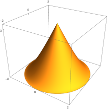
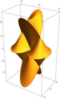
Figure 1. An indefinite improper affine sphere over the region enclosed by . 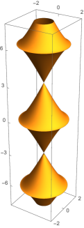
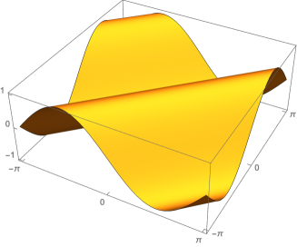
Figure 2. Left: an indefinite improper affine map , which is a series of surfaces in Figure 1, joined along cuspidal edges and at cone points. Right: the graph of , which gives the affine metric of apart from . -
(2)
Second example is given by the square
We have that for , which follows from
where
It is convenient for the following discussion to interpret and for all . It holds for all that
where we denote by the ceiling of , that is, the smallest integer greater than or equal to . Thus we have for that
where
Its data is and
The singular set is a checkerboard
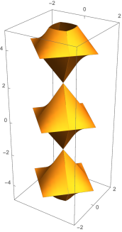
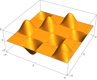
Figure 3. An indefinite improper affine map (left), and its affine metric (right). -
(3)
Last example is given by the curve
We have and hence
(1.38) Therefore
where
Its data is
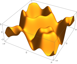
The singular set of is , where
The sets and consist of lines and circlelike curves, respectively. The surface is compact and of genus .
2. Discrete indefinite affine spheres
In the previous section we derived Theorem 1.3 and Corollary 1.8 which offer a Weierstrass type representation formula of indefinite affine spheres. Based on a technique of decompositions of the loop group, we shall generalize this formula to discrete case, and obtain a Weierstrass type representation formula for discrete indefinite affine spheres.
2.1. Definitions
Let be a map. We call a discrete indefinite affine sphere if it satisfies the following two properties ([3], [2], [16]):
-
(1)
Every five points , , lie on a plane.
-
(2)
The line connecting two points and satisfies either of the following two conditions:
-
(a)
All the lines meet at one point in .
-
(b)
All the lines are parallel to each other.
-
(a)
A discrete indefinite affine sphere is said to be proper if it satisfies the condition (2a), or improper if (2b).
If is a discrete indefinite affine sphere, the vector is parallel to the discrete affine normal
| (2.1) |
where is a constant vector. Here we set if is proper, and if is improper. Without loss of generality we can fix to be . Taking into account a continuum limit, we introduce positive numbers and , which play a role of lattice intervals. In view of this it may be better to regard as a map , and hence entries of depend on and . We define
We suppose that , then there exist functions , , such that
| (2.2) | |||
| (2.3) | |||
| (2.4) |
Equations (2.2) and (2.4) are consequences of the property (1). See [3, p. 118] or [16, Proposition 3.4] for a proof. Throughout the paper we further impose on the volume condition
which can be regarded as a discrete analogue of (1.1). We write
| (2.5) |
to have expressions and
From the compatibility condition among (2.2)–(2.4), it follows that , , satisfy the system
| (2.6) | |||
| (2.7) |
Indeed, the matrix varies according to the system
| (2.8) |
where coefficient matrices are computed as
| (2.9) | ||||
| (2.10) |
The compatibility condition is (2.6)–(2.7). Therefore the system (2.8)–(2.10), or equivalently (2.2)–(2.4), has a solution if and only if (2.6)–(2.7) hold. The system (2.6)–(2.7) is a discrete analogue of the system (1.4)–(1.5), and hence called the discrete Tzitzeica equation if , or the discrete Liouville equation if . Since this system (2.6)–(2.7) is invariant under the transformation
the discrete affine sphere has -parameter family, which we call the associated family of . The associated family preserves .
2.2. Loop group description
In order to derive a representation formula for discrete indefinite affine spheres, we use decomposition techniques of loop groups. To begin with, following [3], we describe the discrete indefinite affine spheres in terms of the loop groups. We set
| (2.11) |
Then the map is -valued, and satisfies the system
| (2.12) |
where and are computed as
| (2.13) | ||||
| (2.14) |
The consistency of (2.12), that is, , is of course given by (2.6)–(2.7). By multiplying by some constant matrix from the left if necessary, without loss of generality we can assume that
| (2.15) |
at the base point . The family of gauged frames defined by (2.11) with the initial condition (2.15) will be called the extended frame of discrete affine sphere . The extended frame is obviously a -valued map. Conversely, if the matrices and have similar entries as (2.13) and (2.14) respectively, then they give the extended family of discrete indefinite affine spheres. In fact we have the following proposition, which has been shown for the discrete indefinite proper affine spheres () in [3, Theorem in Section ].
Proposition 2.1.
Let and be matrices which depend on a parameter as
| (2.16) |
Here coefficient matrices and , which are labeled by the index , have the entries
and
with some functions , , and nowhere vanishing functions , , , , and a constant . If and satisfy the relation for all , then there exist a map and a gauge such that
-
(1)
satisfies the system , and
-
(2)
is the extended frame of some discrete indefinite affine sphere.
Proof.
Because of the relation , the existence of is clear. We fix a positive number , and set
Then satisfies and , where
Next we fix a positive number and introduce sequences , , by
and
where is defined by (2.5). Therefore the matrices and are written as
where
We note that the condition is equivalent to
| (2.17) |
which implies that
In fact, comparing the - and -entries of the both sides of (2.17), we have
Then it immediately follows that should be . Further, from - and -entries of (2.17), we have
which implies that . Thus and become exactly the same as (2.13) and (2.14). We conclude that is the extended frame of some discrete indefinite affine sphere. ∎
We are now in position to state one of the main theorems of this paper, which is a discrete analogue of Theorem 1.3.
Theorem 2.2.
Let and be positive numbers, and be the extended frame of a discrete indefinite affine sphere with the discrete affine normal (2.1). By the Birkhoff decomposition, we decompose near as
| (2.18) |
where , , and . Then and do not depend on and , respectively, that is, they satisfy that
We write for and for , so that we have the ordinary difference equations
| (2.19) |
with
| (2.20) | ||||
| (2.21) |
where functions depend only on , and only on . Moreover and for all and .
Conversely, let , be functions depending only on , and , functions depending only on . Assume that and have no zeros. Let and be solutions to the system (2.19)–(2.21) with the initial condition . Define and by the Birkhoff decomposition for near as
| (2.22) |
and write . Then there exists a diagonal matrix such that is the extended frame of a discrete indefinite affine sphere . In particular, in case of discrete indefinite proper affine spheres , the third column of the extended frame directly gives the position vector of .
Proof.
Let be an extended frame, and define and by (2.18). Therefore we have and so that
where is given by (2.14). The left-hand side takes values in and the right-hand side takes values in . Thus . Similarly is identity matrix. Therefore and do not depend on and , respectively.
Next, let us compute and . It is straightforward to see that
where is given by (2.13). Since has the form and takes values in , we have
With the expansions
it is easy to see that , , , are computed as
From Proposition 1.1, every one of , , has the following form
respectively. Since takes values in , thus . Noticing that , , are given by (2.13), it readily follows that the coefficients have the form
where are some functions in . Thus we have
We now consider the twisted condition (1.12), namely . It is easy to see that the twisted condition is equivalent to the system
Thus we have
and the expression (2.20) on rewriting and . We write for the -entry of a matrix , and show that has no zeros as follows. We compute , and so that we have
| (2.23) | ||||
| (2.24) | ||||
| (2.25) |
where we set
Because of the condition , expressions (2.23) and (2.25) imply that has no zeros if . When , expressions (2.24) and (2.25) imply because . Similarly, can be computed as in (2.21) with a nowhere vanishing function .
Conversely, let be a pair of solutions of (2.19) such that . We write
where coefficient matrices and are defined by (2.20) and (2.21). Consider the Birkhoff decomposition of near as and define . We express
Their inverses are
with and , and for all it holds that
Namely the matrices and are computed as
and so forth. Further, from the twisted condition (1.12), it holds that
for all . In particular, setting , we have that
where is some sequence which has no zeros. For higher , we have that
and so on. Here and are some sequences in , . Now we are ready to compute the Maurer-Cartan form of . As for , we have
| (2.26) | ||||
| (2.27) |
Comparing these two expressions, it readily follows that there exist matrices such that
Similarly, from
| (2.28) | ||||
| (2.29) |
we have that
From (2.27) and (2.29), it readily follows that the coefficient matrices are of the form
| (2.30) | |||
| (2.31) |
and is diagonal. On the other hand, from (2.26), we have
| (2.32) | ||||
| (2.33) |
where
Similarly, from (2.28), we have
and hence we have that
| (2.34) | ||||
| (2.35) |
where
For , comparing (2.32) and (2.30), we have , which implies . For , by using (2.27), we have . Comparing (2.33) and (2.30), we have , which implies
For , comparing (2.34) and (2.31), we have , which implies . For , by using (2.29), we have . Comparing (2.35) and (2.31), we have , which implies
Finally, again from (2.27) and (2.29), we have
On the other hand, a straightforward computation shows that -entry of the constant coefficient with respect to for and -entry of the constant coefficient with respect to for can be respectively computed as
Thus and have no zeros near , which implies that and never vanish near .
Remark 2.3.
In case of discrete proper affine spheres , the functions and do not have simple expressions among the functions and . On the other hand, in case of discrete improper affine spheres , they are simply represented as (2.44) below.
2.3. discrete indefinite improper affine spheres
For the rest of this paper, we shall be concerned only with discrete indefinite improper affine spheres . Equations in (2.7) are simplified as
which indicate that and depend only on and , respectively. Hence we write for and for . Thus the discrete Liouville equation (2.6) is written as
| (2.36) |
We now introduce a notation of summation of a sequence as
It holds for all integers that
and hence . In particular we have a formula of summation by parts
| (2.37) |
which holds for all integers . Then the ordinary difference equations (2.19) can be explicitly computed as follows.
Lemma 2.4.
Proof.
Theorem 2.5.
Let , be positive numbers, and , , , be functions in one variable, and , , , be the loops given by (2.38), (2.42), (2.43). Define , , , , , by (2.39), (2.40), and by . We assume that sequences , and have no zeros. Then there exists a diagonal matrix such that is the extended frame of some discrete indefinite improper affine sphere , whose data solving the discrete Liouville equation (2.36) are given as
| (2.44) |
Moreover, the associated family of is given by the representation formula
| (2.45) |
where . All discrete indefinite improper affine spheres are locally constructed in this way.
Proof.
First a straightforward computation shows that Maurer-Cartan form of is computed as
Next we take a diagonal gauge so that the Maurer-Cartan form of is
This should be compared with (2.13)–(2.14) with , thus we have (2.44) and
To obtain the formula (2.45), we consider another diagonal gauge as introduced in (2.11). Namely, setting where , we have
| (2.46) | ||||
| (2.47) |
Of course this pair of matrices accords with (2.9) and (2.10). The frame can be computed explicitly as
where
By definition of the moving frame, we have
Hence, noticing (2.37), and the relations
and , it follows for all integers and that
Thus we have the representation formula (2.45) up to equiaffine transformations. ∎
Remark 2.6.
For given functions , and positive constants , , it is known that a general solution to the discrete Liouville equation (2.36) can be expressed as
where and are arbitrary functions with no zeros in one variable, and and are arbitrary constants. See, for example, [24]. On the other hand, our formula (2.44) tells that a general solution also has an expression
where and are arbitrary functions with no zeros in one variable. As the most simple solutions, by setting and , these formulas give an additive one and a multiplicative one , respectively.
We conclude this paper with one of our main results, which offers a representation formula using two discrete plane curves for a discrete indefinite improper affine sphere.
Corollary 2.7 (Representation formula).
Fix positive numbers and . For maps and , set
Then the map
| (2.48) |
where
| (2.49) |
is a discrete indefinite improper affine sphere with the affine normal . Its data solving the discrete Liouville equation (2.36) is
Moreover the associated family of is given by the transformation
where . Conversely all discrete indefinite improper affine spheres can be constructed in this way.
Proof.
First, introducing functions and , we rephrase (2.45) as
| (2.50) |
where we use the identities
and . Note that . We then consider an equiaffine transformation of as
where , , and are some constants. A straightforward computation shows that
where , , and . Thus we obtain (2.48) on writing
Since and are arbitrary, (2.48) gives the all improper indefinite affine spheres. ∎
Remark 2.8.
We recall that the height function defined by (1.31) satisfies . As a discrete analogue of this, the sequence defined by (2.49) satisfies a difference equation
| (2.51) |
In particular, if and for all , then satisfies for all , and then every can be fast computed by using the recurrent relation (2.51). Iterating this, we can obtain all the values numerically. Refer to Example 4 for specific examples, where we explicitly calculate as a function in .
We fix positive numbers and arbitrarily to illustrate examples of discrete indefinite improper affine spheres by taking several discrete curves.
Example 3.
Let and be arbitrary sequences which possibly depend on and respectively. We denote by and the forward differences of them, that is,
We substitute discrete curves
into the representation formula (2.48), and have a discrete indefinite improper affine sphere
Its data is
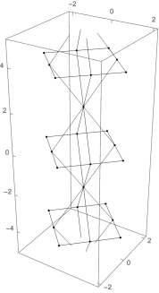
Example 4.
We illustrate discrete counterparts to those surfaces given in Example 2. Fix positive numbers , arbitrarily and introduce positive numbers
-
(1)
First example is given by the discrete curves
Substituting these into the representation formula, we have
The data solving the discrete Liouville equation (2.36) are given by constants
and a sequence
Therefore is singular if , satisfy


(a) 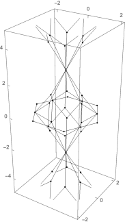
(b) 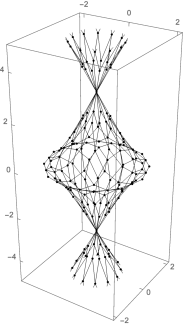
(c) Figure 5. Discrete indefinite improper affine spheres with and , which exhibit cone points. The figures in upper line show views from the top. -
(2)
Second example is given by
We assume that both the images of and contain four points
which we can always achieve by choosing , appropriately. By virtue of this assumption, we are able to assume that and and . Therefore the differences of can be written into simple forms as
Hence we have that
Further, on choosing the parameter as
with a positive integer , which is equivalent to setting , it holds for all that
Here is the floor of , that is, the greatest integer less than or equal to . We apply the same discussion as above to , and set to have
Its data is
The singular set consists of integer points in a checkerboard, that is
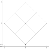

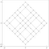
(a) 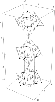
(b) 
(c) Figure 6. Discrete indefinite improper affine spheres with and . The figures in upper line show views from the top. -
(3)
Third example is given by
We have
and hence
Here the coefficients are given as
This should be compared with (1.38). We have
where
Its data is given as
where
and
Especially if we choose the parameters , so as to be
with a positive integer , then is factorized as
The singular set is given by
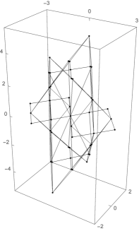
(a) 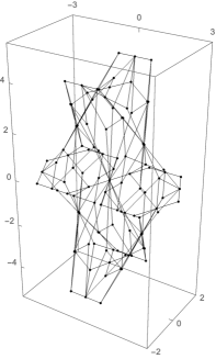
(b) 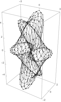
(c) Figure 7. Discrete indefinite improper affine spheres with .
References
- [1] Wilhelm Blaschke, Vorlesungen über Differentialgeometrie und geometrische Grundlagen von Einsteins Relativitätstheorie. Band II. Affine Differentialgeometrie, Berlin, Verlag von Julius Springer, 1923.
- [2] Alexander I. Bobenko and Wolfgang K. Schief, Affine spheres: discretization via duality relations, Experiment. Math. 8 (1999), no. 3, 261–280. MR 1724159
- [3] by same author, Discrete indefinite affine spheres, Discrete integrable geometry and physics (Vienna, 1996), Oxford Lecture Ser. Math. Appl., vol. 16, Oxford Univ. Press, New York, 1999, pp. 113–138. MR 1676596
- [4] Alexander I. Bobenko and Yuri B. Suris, Discrete differential geometry, Graduate Studies in Mathematics, vol. 98, American Mathematical Society, Providence, RI, 2008, Integrable structure. MR 2467378 (2010f:37125)
- [5] Marcos Craizer, Moacyr Alvim, and Ralph Teixeira, Area distances of convex plane curves and improper affine spheres, SIAM J. Imaging Sci. 1 (2008), no. 3, 209–227. MR 2486030
- [6] Marcos Craizer, Ralph C. Teixeira, and Moacyr A. H. B. da Silva, A geometric representation of improper indefinite affine spheres with singularities, J. Geom. 100 (2011), no. 1-2, 65–78. MR 2845277
- [7] R. K. Dodd and R. K. Bullough, Polynomial conserved densities for the sine-Gordon equations, Proc. Roy. Soc. London Ser. A 352 (1977), no. 1671, 481–503. MR 0442516
- [8] J. Dorfmeister and U. Eitner, Weierstraß-type representation of affine spheres, Abh. Math. Sem. Univ. Hamburg 71 (2001), 225–250. MR 1873045
- [9] Roland Hildebrand, Canonical barriers on convex cones, Math. Oper. Res. 39 (2014), no. 3, 841–850. MR 3247006
- [10] Ryogo Hirota, Nonlinear partial difference equations. V. Nonlinear equations reducible to linear equations, J. Phys. Soc. Japan 46 (1979), 312–319.
- [11] Go-O Ishikawa and Yoshinori Machida, Singularities of improper affine spheres and surfaces of constant Gaussian curvature, Internat. J. Math. 17 (2006), no. 3, 269–293. MR 2215151
- [12] O. V. Kaptsov and Yu. V. Shan′ ko, Multiparametric solutions of the Tzitzeica equation, Differ. Uravn. 35 (1999), no. 12, 1660–1668, 1726. MR 1774990
- [13] Shimpei Kobayashi, Nonlinear d’Alembert formula for discrete pseudospherical surfaces, J. Geom. Phys. 119 (2017), 208–223. MR 3661533
- [14] Igor Moiseevich Krichever, An analogue of the d’Alembert formula for the equations of a principal chiral field and the sine-Gordon equation, Dokl. Akad. Nauk SSSR 253 (1980), no. 2, 288–292. MR 581396
- [15] A. Martínez, Improper affine maps, Math. Z. 249 (2005), no. 4, 755–766. MR 2126213
- [16] Nozomu Matsuura and Hajime Urakawa, Discrete improper affine spheres, J. Geom. Phys. 45 (2003), no. 1-2, 164–183. MR 1949349
- [17] Alexander V. Mikhailov, The reduction problem and the inverse scattering method, Physica D: Nonlinear Phenomena 3 (1981), no. 1, 73 – 117.
- [18] Daisuke Nakajo, A representation formula for indefinite improper affine spheres, Results Math. 55 (2009), no. 1-2, 139–159. MR 2546487
- [19] J. J. C. Nimmo and R. Willox, Darboux transformations for the two-dimensional Toda system, Proc. Roy. Soc. London Ser. A 453 (1997), no. 1967, 2497–2525. MR 1490247
- [20] Franz Pedit and Hongyou Wu, Discretizing constant curvature surfaces via loop group factorizations: the discrete sine- and sinh-Gordon equations, J. Geom. Phys. 17 (1995), no. 3, 245–260. MR 97a:39022
- [21] Helmut Pottmann, Sigrid Brell-Cokcan, and Johannes Wallner, Discrete surfaces for architectural design, Curve and surface design: Avignon 2006, Mod. Methods Math., Nashboro Press, Brentwood, TN, 2007, pp. 213–234. MR 2335142
- [22] Andrew Pressley and Graeme Segal, Loop groups, Oxford Mathematical Monographs, The Clarendon Press, Oxford University Press, New York, 1986, Oxford Science Publications. MR 900587
- [23] W. K. Schief, Hyperbolic surfaces in centro-affine geometry. Integrability and discretization, Chaos Solitons Fractals 11 (2000), no. 1-3, 97–106, Integrability and chaos in discrete systems (Brussels, 1997). MR 1729560
- [24] C. Scimiterna, B. Grammaticos, and A. Ramani, On two integrable lattice equations and their interpretation, J. Phys. A 44 (2011), no. 3, 032002, 6. MR 2749061
- [25] Georges Tzitzéica, Sur une nouvelle classe de surfaces, C. R. Acad. Sci. 144 (1907), 1257–1259.
- [26] by same author, Sur une nouvelle classe de surfaces, C. R. Acad. Sci. 146 (1908), 165–166.
- [27] by same author, Sur une nouvelle classe de surfaces, Rend. Circ. Mat. Palermo 25 (1908), 180–187.
- [28] by same author, Sur une nouvelle classe de surfaces, Rend. Circ. Mat. Palermo 28 (1909), 210–216.
- [29] by same author, Sur une nouvelle classe de surfaces, C. R. Acad. Sci. 150 (1910), 955–956.
- [30] by same author, Sur une nouvelle classe de surfaces, C. R. Acad. Sci. 150 (1910), 1227–1229.
- [31] A. V. ˇZiber and A. B. ˇSabat, The Klein-Gordon equation with nontrivial group, Dokl. Akad. Nauk SSSR 247 (1979), no. 5, 1103–1107. MR 550472