From abstract items to latent spaces to observed data and back: Compositional Variational Auto-Encoder

Abstract

Conditional Generative Models are now acknowledged an essential tool in Machine Learning. This paper focuses on their control. While many approaches aim at disentangling the data through the coordinate-wise control of their latent representations, another direction is explored in this paper. The proposed CompVAE handles data with a natural multi-ensemblist structure (i.e. that can naturally be decomposed into elements). Derived from Bayesian variational principles, CompVAE learns a latent representation leveraging both observational and symbolic information. A first contribution of the approach is that this latent representation supports a compositional generative model, amenable to multi-ensemblist operations (addition or subtraction of elements in the composition). This compositional ability is enabled by the invariance and generality of the whole framework w.r.t. respectively, the order and number of the elements. The second contribution of the paper is a proof of concept on synthetic 1D and 2D problems, demonstrating the efficiency of the proposed approach.

Keywords: Generative model, semi-structured representation, neural networks

1 Introduction

Representation learning is at the core of machine learning, and even more so since the inception of deep learning [2]. As shown by e.g., [3, 12], the latent representations built to handle high-dimensional data can effectively support desirable functionalities. One such functionality is the ability to directly control the observed data through the so-called representation disentanglement, especially in the context of computer vision and image processing [25, 20] (more in section 2).

This paper extends the notion of representation disentanglement from a latent coordinate-wise perspective to a semi-structured setting. Specifically, we tackle the ensemblist setting where a datapoint can naturally be interpreted as the combination of multiple parts. The contribution of the paper is a generative model built on the Variational Auto-Encoder principles [17, 27], controlling the data generation from a description of its parts and supporting ensemblist operations such as the addition or removal of any number of parts.

The applicative motivation for the presented approach, referred to as Compositional Variational AutoEncoder (CompVAE), is the following. In the domain of Energy Management, a key issue is to simulate the consumption behavior of an ensemble of consumers, where each household consumption is viewed as an independent random variable following a distribution law defined from the household characteristics, and the household consumptions are possibly correlated through external factors such as the weather, or a football match on TV (attracting members of some but not all households). Our long term goal is to infer a simulator, taking as input the household profiles and their amounts: it should be able to simulate their overall energy consumption and account for their correlations. The data-driven inference of such a programmable simulator is a quite desirable alternative to the current approaches, based on Monte-Carlo processes and requiring either to explicitly model the correlations of the elementary random variables, or to proceed by rejection.

Formally, given the description of datapoints and their parts, the goal of CompVAE is to learn the distribution laws of the parts (here, the households) and to sample the overall distribution defined from a varying number of parts (the set of households), while accounting for the fact that the parts are not independent, and the sought overall distribution depends on shared external factors: the whole is not the sum of its parts.

The paper is organized as follows. Section 2 briefly reviews related work in the domain of generative models and latent space construction, replacing our contribution in context. Section 3 gives an overview of CompVAE, extending the VAE framework to multi-ensemblist settings. Section 4 presents the experimental setting retained to establish a proof of concept of the approach on two synthetic problems, and section 5 reports on the results. Finally section 6 discusses some perspectives for further work and applications to larger problems.

2 Related Work

Generative models, including VAEs [17, 27] and GANs [9], rely on an embedding from the so-called latent space $Z$ onto the dataspace $X$. In the following, data space and observed space are used interchangeably. It has long been observed that continuous or discrete operations in the latent space could be used to produce interesting patterns in the data space. For instance, the linear interpolation between two latent points $z$ and $z^{\prime}$ can be used to generate a morphing between their images [26], or the flip of a boolean coordinate of $z$ can be used to add or remove an elementary pattern (the presence of glasses or mustache) in the associated image [7].

The general question then is to control the flow of information from the latent to the observed space and to make it actionable. Several approaches, either based on information theory or on supervised learning have been proposed to do so. Losses inspired from the Information Bottleneck [31, 29, 1] and enforcing the independence of the latent and the observed variables, conditionally to the relevant content of information, have been proposed: enforcing the decorrelation of the latent coordinates in $\beta$-VAE [12]; aligning the covariances of latent and observed data in [19]; decomposing the latent information into pure content and pure noise in InfoGAN [3]. Independently, explicit losses have been used to yield conditional distributions in conditional GANs [23], or to enforce the scope of a latent coordinate in [18, 32], (e.g. modeling the light orientation or the camera angle).

The structure of the observed space can be mimicked in the latent space, to afford expressive yet trainable model spaces; in Ladder-VAE [30], a sequence of dependent latent variables are encoded and reversely decoded to produce complex observed objects. Auxiliary losses are added in [22] in the spirit of semi-supervised learning. In [16], the overall generative model involves a classifier, trained both in a supervised way with labeled examples and in an unsupervised way in conjunction with a generative model.

An important case study is that of sequential structures: [5] considers fixed-length sequences and loosely mimics an HMM process, where latent variable $z_{\_}i$ controls the observed variable $x_{\_}i$ and the next latent $z_{\_}{i+1}$. In [13], a linear relation among latent variables $z_{\_}i$ and $z_{\_}{i+1}$ is enforced; in [6], a recurrent neural net is used to produce the latent variable encoding the current situation. In a more general context, [34] provides a generic method for designing an appropriate inference network that can be associated with a given Bayesian network representing a generative model to train.

The injection of explicit information at the latent level can be used to support ”information surgery” via loss-driven information parsimony. For instance in the domain of signal generation [4], the neutrality of the latent representation w.r.t. the locutor identity is enforced by directly providing the identity at the latent level: as $z$ does not need to encode the locutor information, the information parsimony pressure ensures $z$ independence wrt the locutor. Likewise, fair generative processes can be enforced by directly providing the sensitive information at the latent level [35]. In [21], an adversarial mechanism based on Maximum Mean Discrepancy [10] is used to enforce the neutrality of the latent. In [24], the minimization of the mutual information is used in lieu of an adversary.

Discussion.

All above approaches (with the except of sequential settings [5, 13], see below) handle the generation of a datapoint as a whole naturally involving diverse facets; but not composed of inter-related parts. Our goal is instead to tackle the proper parts-and-whole structure of a datapoint, where the whole is not necessarily the simple sum of its parts and the parts of the whole are interdependent. In sequential settings [5, 13], the dependency of the elements in the sequence are handled through parametric restrictions (respectively considering fixed sequence-size or linear temporal dependency) to enforce the proper match of the observed and latent spaces. A key contribution of the proposed CompVAE is to tackle the parts-to-whole structure with no such restrictions, and specifically accommodating a varying number of parts $-$ possibly different between the training and the generation phases.

3 Overview of CompVAE

This section describes the CompVAE model, building upon the VAE principles [17] with the following difference: CompVAE aims at building a programmable generative model $p_{\_}\theta$, taking as input the ensemble of the parts of a whole observed datapoint. A key question concerns the latent structure most appropriate to reflect the ensemblist nature of the observed data. The proposed structure (section 3.1) involves a latent variable associated to each part of the whole. The aggregation of the part is achieved through an order-invariant operation, and the interactions among the parts are modeled at an upper layer of the latent representation.

In encoding mode, the structure is trained from the pairs formed by a whole, and an abstract description of its parts; the latent variables are extracted along an iterative non-recurrent process, oblivious of the order and number of the parts (section 3.2) and defining the encoder model $q_{\_}\phi$.
In generative mode, the generative model is supplied with a set of parts, and accordingly generates a consistent whole, where variational effects operate jointly at the part and at the whole levels.

Notations.

A datapoint $x$ is associated with an ensemble of parts noted $\{\ell_{\_}i\}$. Each $\ell_{\_}i$ belongs to a finite set of categories $\Lambda$. Elements and parts are used interchangeably in the following. In our illustrating example, a consumption curve $x$ involves a number of households; the $i$-th household is associated with its consumer profile $\ell_{\_}i$, with $\ell_{\_}i$ ranging in a finite set of profiles. Each profile in $\Lambda$ thus occurs 0, 1 or several times. The generative model relies on a learned distribution $p_{\_}\theta(x|\{\ell_{\_}i\})$, that is decomposed into latent variables: a latent variable named $w_{\_}i$ associated to each part $\ell_{\_}i$, and a common latent variable $z$.

Figure 1: Bayesian network representation of the CompVAE generative model.

3.1 CompVAE: Bayesian architecture

The architecture proposed for CompVAE is depicted as a graphical model on Fig. 1. As said, the $i$-th part belongs to category $\ell_{\_}i$ and is associated with a latent variable $w_{\_}i$ (different parts with same category are associated with different latent variables). The ensemble of the $w_{\_}i$s is aggregated into an intermediate latent variable $\widetilde{w}$. A key requirement is for $\widetilde{w}$ to be invariant w.r.t. the order of elements in $x$. In the following $\widetilde{w}$ is set to the sum of the $w_{\_}i$, ${\mbox{$\widetilde{w}$}}=\sum_{\_}iw_{\_}i$. Considering other order-invariant aggregations is left for further work.
The intermediate latent variable $\widetilde{w}$ is used to condition the $z$ latent variable; both $\widetilde{w}$ and $z$ condition the observed datapoint $x$. This scheme corresponds to the following factorization of the generative model $p_{\_}\theta$:

$$p_{\_}\theta(x,z,\{w_{\_}i\}|\{\ell_{\_}i\})=p_{\_}\theta(x|z,{\mbox{$\widetilde{w}$}})p_{\_}\theta(z|{\mbox{$\widetilde{w}$}})\prod_{\_}ip_{\_}\theta(w_{\_}i|\ell_{\_}i)$$ (1)

In summary, the distribution of $x$ is conditioned on the ensemble $\{\ell_{\_}i\}$ as follows: The $i$-th part of $x$ is associated with a latent variable $w_{\_}i$ modeling the generic distribution of the underlying category $\ell_{\_}i$ together with its specifics. Variable $\widetilde{w}$ is deterministically computed to model the aggregation of the $w_{\_}i$, and finally $z$ models the specifics of the aggregation.

Notably, each $w_{\_}i$ is linked to a single $\ell_{\_}i$ element, while $z$ is global, being conditioned from the global auxiliary $\widetilde{w}$. The rationale for introducing $z$ is to enable a more complex though still learnable distribution at the $x$ level $-$ compared with the alternative of conditioning $x$ only on $\widetilde{w}$. It is conjectured that an information-effective distribution would store in $w_{\_}i$ (respectively in $z$) the local information related to the $i$-th part (resp. the global information describing the interdependencies between all parts, e.g. the fact that the households face the same weather, vacation schedules, and so on). Along this line, it is conjectured that the extra information stored in $z$ is limited compared to that stored in the $w_{\_}i$s; we shall return to this point in section 4.1.

The property of invariance of the distribution w.r.t. the order of the $\ell_{\_}i$ is satisfied by design. A second desirable property regards the robustness of the distribution w.r.t. the varying number of parts in $x$. More precisely, two requirements are defined. The former one, referred to as size-flexibility property, is that the number $K$ of parts of an $x$ is neither constant, nor bounded a priori. The latter one, referred to as size-generality property is the generative model $p_{\_}\theta$ to accommodate larger numbers of parts than those seen in the training set.

3.2 Posterior inference and loss

Letting $p_{\_}D(x|\{\ell_{\_}i\})$ denote the empirical data distribution, the learning criterion to optimize is the data likelihood according to the sought generative model $p_{\_}\theta$: $\operatorname*{\mathbb{E}}_{\_}{p_{\_}D}\log p_{\_}\theta(x|\{\ell_{\_}i\})$.
The (intractable) posterior inference of the model is approximated using the Evidence Lower Bound (ELBO) [14], following the Variational AutoEncoder approach [17, 27]. Accordingly, we proceed by optimizing a lower bound of the log-likelihood of the data given $p_{\_}\theta$, which is equivalent to minimizing an upper bound of the Kullback-Leibler divergence between the two distributions :

$$D_{\_}{KL}(p_{\_}D\|p_{\_}\theta)\leq H(p_{\_}D)+\operatorname*{\mathbb{E}}_{\_}{x\sim p_{\_}D}\mathcal{L}_{\_}{ELBO}(x)$$ (2)

The learning criterion is, with $q_{\_}\phi(z,\{w_{\_}i\}|x,\{\ell_{\_}i\})$ the inference distribution:

$$\begin{split}\mathcal{L}_{\_}{ELBO}(x)&=\operatorname*{\mathbb{E}}_{\_}{z,\{w_{\_}i\}\sim q_{\_}\phi}\log\frac{q_{\_}\phi(z,\{w_{\_}i\}|x,\{\ell_{\_}i\})}{p_{\_}\theta(z|{\mbox{$\widetilde{w}$}})\prod_{\_}ip_{\_}\theta(w_{\_}i|\ell_{\_}i)}\\ &-\operatorname*{\mathbb{E}}_{\_}{z,\{w_{\_}i\}\sim q_{\_}\phi}\log p_{\_}\theta(x|z,{\mbox{$\widetilde{w}$}})\end{split}$$ (3)

The inference distribution is further factorized as $q_{\_}\phi(\{w_{\_}i\}|z,x,\{l_{\_}i\})q_{\_}\phi(z|x)$, yielding the final training loss:

$$\begin{split}\mathcal{L}_{\_}{ELBO}(x)&=\operatorname*{\mathbb{E}}_{\_}{z,\{w_{\_}i\}\sim q_{\_}\phi}\log\frac{q_{\_}\phi(\{w_{\_}i\}|x,z,\{\ell_{\_}i\})}{\prod_{\_}ip_{\_}\theta(w_{\_}i|\ell_{\_}i)}\\ &+\operatorname*{\mathbb{E}}_{\_}{z,\{w_{\_}i\}\sim q_{\_}\phi}\log\frac{q_{\_}\phi(z|x)}{p_{\_}\theta(z|{\mbox{$\widetilde{w}$}})}\\ &-\operatorname*{\mathbb{E}}_{\_}{z,\{w_{\_}i\}\sim q_{\_}\phi}\log p_{\_}\theta(x|z,{\mbox{$\widetilde{w}$}})\end{split}$$ (4)

The training of the generative and encoder model distributions is described in Alg. 1.

$\theta,\phi\leftarrow\text{Random initialization}$;

while Not converged do

       $x,\{\ell_{\_}i\}\leftarrow\text{Sample minibatch}$;

       $z\leftarrow\text{Sample from\ }q_{\_}\phi(z|x)$;

       $\{w_{\_}i\}\leftarrow\text{Sample from\ }q_{\_}\phi(\{w_{\_}i\}|x,z,\{\ell_{\_}i\})$;

       $\mathcal{L}_{\_}w\leftarrow D_{\_}{KL}(q_{\_}\phi(\{w_{\_}i\}|x,z,\{\ell_{\_}i\})\|\Pi_{\_}ip_{\_}\theta(w_{\_}i|\ell_{\_}i))$;

       $\mathcal{L}_{\_}z\leftarrow\log\frac{q_{\_}\phi(z|x)}{p_{\_}\theta(z|\tilde{w})}$;

       $\mathcal{L}_{\_}x\leftarrow-\log p_{\_}\theta(x|z,\tilde{w})$;

       $\mathcal{L}_{\_}{ELBO}\leftarrow\mathcal{L}_{\_}w+\mathcal{L}_{\_}z+\mathcal{L}_{\_}x$;

       $\theta\leftarrow\text{Update}(\theta,\nabla_{\_}\theta\mathcal{L}_{\_}{ELBO})$;

       $\phi\leftarrow\text{Update}(\phi,\nabla_{\_}\phi\mathcal{L}_{\_}{ELBO})$;

      

end while

Algorithm 1 CompVAE Training Procedure.

3.3 Discussion

In CompVAE, the sought distributions are structured as a Bayesian graph (see $p_{\_}\theta$ in Fig. 1), where each node is associated with a neural network and a probability distribution family, like for VAEs. This neural network takes as input the parent variables in the Bayesian graph, and outputs the parameters of a distribution in the chosen family, e.g., the mean and variance of a Gaussian distribution. The reparametrization trick [17] is used to back-propagate gradients through the sampling.

A concern regards the training of latent variables when considering Gaussian distributions. A potential source of instability in CompVAE comes from the fact that the Kullback-Leibler divergence between $q_{\_}\phi$ and $p_{\_}\theta$ (Eq. (4)) becomes very large when the variance of some variables in $p_{\_}\theta$ becomes very small. To limit this risk, some care is exercised in parameterizing the variances of the normal distributions in $p_{\_}\theta$ to making them lower-bounded.

3.3.1 Modeling of $q_{\_}\phi(\{w_{\_}i\}|x,z,\{\ell_{\_}i\})$.

The latent distributions $p_{\_}\theta(z|{\mbox{$\widetilde{w}$}})$, $p_{\_}\theta(w_{\_}i|\ell_{\_}i)$ and $q_{\_}\phi(z|x)$ are modeled using diagonal normal distributions as usual. Regarding the model $q_{\_}\phi(\{w_{\_}i\}|z,x,\{\ell_{\_}i\})$, in order to be able to faithfully reflect the generative model $p_{\_}\theta$, it is necessary to introduce the correlation between the $w_{\_}i$s in $q_{\_}\phi(\{w_{\_}i\}|z,x,\{\ell_{\_}i\})$ [34].

As the aggregation of the $w_{\_}i$ is handled by considering their sum, it is natural to handle their correlations through a multivariate normal distribution over the $w_{\_}i$. The proposed parametrization of such a multivariate is as follows. Firstly, correlations operate in a coordinate-wise fashion, that is, $w_{\_}{i,j}$ and $w_{\_}{i^{\prime},j^{\prime}}$ are only correlated if $j=j^{\prime}$. The parametrization (detailed in appendix LABEL:app:multivariate-parameter) of the $w_{\_}i$s ensures that: i) the variance of the sum of the $w_{\_}{i,j}$ can be controlled and made arbitrarily small in order to ensure an accurate VAE reconstruction; ii) the Kullback-Leibler divergence between $q_{\_}\phi(\{w_{\_}i\}|x,z,\{\ell_{\_}i\})$ and $\prod_{\_}ip_{\_}\theta(w_{\_}i|\ell_{\_}i)$ can be defined in closed form.

The learning of $q_{\_}\phi(\{w_{\_}i\}|x,z,\{\ell_{\_}i\})$ is done using a fully-connected graph neural network [28] leveraging graph interactions akin message-passing [8]. The graph has one node for each element $\ell_{\_}i$, and every node is connected to all other nodes. The state of the $i$-th node is initialized to $(pre_{\_}\phi(x),z,e_{\_}\phi(\ell_{\_}i)+\epsilon_{\_}i)$, where $pre_{\_}\phi(x)$ is some learned function of $x$ noted, $e_{\_}\phi(\ell_{\_}i)$ is a learned embedding of $\ell_{\_}i$, and $\epsilon_{\_}i$ is a random noise used to ensure the differentiation of the $w_{\_}i$s. The state of each node of the graph at the $k$-th layer is then defined by its $k-1$-th layer state and the aggregation of the state of all other nodes:

$$\begin{cases}h_{\_}i^{(0)}=(pre_{\_}\phi(x),z,e_{\_}\phi(\ell_{\_}i)+\epsilon_{\_}i)\\ h_{\_}i^{(k)}=f_{\_}\phi^{(k)}\left(h_{\_}i^{(k-1)},\sum_{\_}{j\neq i}g_{\_}\phi^{(k)}(h_{\_}j^{(k-1)})\right)\end{cases}$$ (5)

where $f_{\_}\phi^{(k)}$ and $g_{\_}\phi^{(k)}$ are learned neural networks: $g_{\_}\phi^{(k)}$ is meant to embed the current state of each node for an aggregate summation, and $f_{\_}\phi^{(k)}$ is meant to ”fine-tune” the $i$-th node conditionally to all other nodes, such that they altogether account for $\widetilde{w}$.

4 Experimental Setting

This section presents the goals of experiments and describes the experimental setting used to empirically validate CompVAE.

4.1 Goals of experiments

As said, CompVAE is meant to achieve a programmable generative model. From a set of latent values $w_{\_}i$, either derived from $p_{\_}\theta(w_{\_}i|\ell_{\_}i)$ in a generative context, or recovered from some data $x$, it should be able to generate values $\hat{x}$ matching any chosen subset of the $w_{\_}i$. This property is what we name the ”ensemblist disentanglement” capacity, and the first goal of these experiments is to investigate whether CompVAE does have this capacity.

A second goal of these experiments is to examine whether the desired properties (section 3.1) hold. The order-invariant property is enforced by design. The size-flexibility property will be assessed by inspecting the sensitivity of the extraction and generative processes to the variability of the number of parts. The size-generality property will be assessed by inspecting the quality of the generative model when the number of parts increases significantly beyond the size range used during training.

A last goal is to understand how CompVAE manages to store the information of the model in respectively the $w_{\_}i$s and $z$. The conjecture done (section 3.1) was that the latent $w_{\_}i$s would take in charge the information of the parts, while the latent $z$ would model the interactions among the parts. The use of synthetic problems where the quantity of information required to encode the parts can be quantitatively assessed will permit to test this conjecture. A related question is whether the generative model is able to capture the fact that the whole is not the sum of its parts. This question is investigated using non-linear perturbations, possibly operating at the whole and at the parts levels, and comparing the whole perturbed $x$ obtained from the $\ell_{\_}i$s, and the aggregation of the perturbed $x_{\_}i$s generated from the $\ell_{\_}i$ parts. The existence of a difference, if any, will establish the value of the CompVAE generative model compared to a simple Monte-Carlo simulator, independently sampling parts and thereafter aggregating them.

4.2 1D and 2D Proofs of concept

Two synthetic problems have been considered to empirically answer the above questions.

In the 1D synthetic problem,

the set $\Lambda$ of categories is a finite set of frequencies $\lambda_{\_}1\ldots\lambda_{\_}{10}$. A given ”part” (here, curve) is a sine wave defined by its frequency $\ell_{\_}i$ in $\Lambda$ and its intrinsic features, that is, its amplitude $a_{\_}i$ and phase $\kappa_{\_}i$. The whole $x$ associated to $\{\ell_{\_}1,\ldots\ell_{\_}K\}$ is a finite sequence of size $T$, deterministically defined from the non-linear combination of the curves:

$$x(t)=K\tanh\left(\frac{{\mbox{$C$}}}{K}\sum_{\_}{i=0}^{K}a_{\_}i\cos\left(\frac{2\pi\ell_{\_}i}{T}t+\kappa_{\_}i\right)\right)$$

with $K$ the number of sine waves in $x$, $C$  a parameter controlling the non-linearity of the aggregation of the curves in $x$, and $T$ a global parameter controlling the sampling frequency. For each part (sine wave), $a_{\_}i$ is sampled from $\mathcal{N}(1;0.3)$, and $\kappa_{\_}i$ is sampled from $\mathcal{N}\left(0;\frac{\pi}{2}\right)$.

The part-to-whole aggregation is illustrated on Fig. 2, plotting the non-linear transformation of the sum of 4 sine waves, compared to the sum of non-linear transformations of the same sine waves. The sensitivity to $C$ is illustrated in supplementary material (Appendix LABEL:app:data-generation Fig. LABEL:fig:lambda-impact). $C$ is set to 3 in the experiments.

Figure 2: Non-linear part-to-whole aggregation (purple) compared to the sum of non-linear perturbations of the parts (green). Better seen in color. Both curves involve a non-linear transform factor ${\mbox{$C$}}=3$.

This 1D synthetic problem features several aspects relevant to the empirical assessment of CompVAE. Firstly, the impact of adding or removing one part can be visually assessed as it changes the whole curve: the general magnitude of the whole curve is roughly proportional to its number of parts. Secondly, each part involves, besides its category $\ell_{\_}i$, some intrinsic variations of its amplitude and phase. Lastly, the whole $x$ is not the sum of its parts (Fig. 2).

The generative model $p_{\_}\theta(x|z,\sum_{\_}iw_{\_}i)$ is defined as a Gaussian distribution $\mathcal{N}(\mu;\Delta(\sigma))$, the vector parameters $\mu$ and $\sigma$ of which are produced by the neural network (architecture details in supplementary material, section LABEL:app:sines-nn-structure).

In the 2D synthetic problem,

each category in $\Lambda$ is composed of one out of five colors ($\{red,green,$ $blue,white,black\}$) associated with a location $(x,y)$ in $[0,1]\times[0,1]$. Each $\ell_{\_}i$ thus is a colored site, and its internal variability is its intensity. The whole $x$ associated to a set of $\ell_{\_}i$s is an image, where each pixel is colored depending on its distance to the sites and their intensity (Fig. 3).

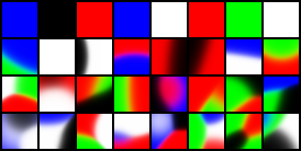
Figure 3: 2D visual synthetic examples, including 1 to 4 sites (top to bottom). Note that when neighbor sites have same color, the image might appear to have been generated with less sites than it actually has.

Likewise, the observation model $p_{\_}\theta(x|z,\sum_{\_}iw_{\_}i)$ is a Gaussian distribution $\mathcal{N}(\mu;\Delta(\sigma))$, the parameters $\mu$ and $\sigma$ of which are produced by the neural network. The observation variance is shared for all three channel values (red, green, blue) of any given pixel. Architecture details are given in supplementary material (section LABEL:app:dots-nn-structure).

The 2D problem shares with the 1D problem the fact that each part is defined from its category $\ell_{\_}i$ (resp. a frequency, or a color and location) on the one hand, and its specifics on the other hand (resp, its amplitude and frequency, or its intensity); additionally, the whole is made of a set of parts in interaction. However, the 2D problem is significantly more complex than the 1D, as will be discussed in section 5.2.

4.3 Experimental setting

CompVAE is trained as a mainstream VAE, except for an additional factor of difficulty: the varying number of latent variables (reflecting the varying number of parts) results in a potentially large number of latent variables. This large size and the model noise in the early training phase can adversely affect the training procedure, and lead it to diverge. The training divergence is prevented using a batch size set to 256. The neural training hyperparameters are dynamically tuned using the Adam optimizer [15] with $\alpha=10^{-4}$, $\beta_{\_}1=0.5$ and $\beta_{\_}2=0.9$, which empirically provide a good compromise between training speed, network stability and good convergence. On the top of Adam, the annealing of the learning rate $\alpha$ is achieved, dividing its value by 2 every 20,000 iterations, until it reaches $10^{-6}$.

For both problems, the data is generated on the fly during the training, preventing the risk of overfitting. The overall number of iterations (batches) is up to 500,000. The computational time on a GPU GTX1080 is 1 day for the 1D problem, and 2 days for the 2D problem.

Empirically, the training is facilitated by gradually increasing the number $K$ of parts in the datapoints. Specifically, the number of parts is uniformly sampled in $[[1,K]]$ at each iteration, with $K=2$ at the initialization and $K$ incremented by 1 every 3,000 iterations, up to 16 parts in the 1D problem and 8 in the 2D problem.

5 CompVAE: Empirical Validation

This section reports on the proposed proofs of concept of the CompVAE approach.

5.1 1D Proof of Concept

Fig. 4 displays in log-scale the losses of the $w_{\_}i$s and $z$ latent variables along time, together with the reconstruction loss and the overall ELBO loss summing the other three (Eq. (4)). The division of labor between the $w_{\_}i$s and the $z$ is seen as the quantity of information stored by the $w_{\_}i$s increases to reach a plateau at circa 100 bits, while the quantity of information stored by $z$ steadily decreases to around 10 bits. As conjectured (section 3.1), $z$ carries little information.

Figure 4: CompVAE, 1D problem: Losses of the latent variables respectively associated to the parts ($w_{\_}i$, green), to the whole ($z$, blue), and the reconstruction loss of $x$ (yellow), in log scale. Better seen in color.

Note that the $x$ reconstruction loss remains high, with a high ELBO even at convergence time, although the generated curves ”look good”. This fact is explained from the high entropy of the data: on the top of the specifics of each part (its amplitude and phase), $x$ is described as a $T$-length sequence: the temporal discretization of the signal increases the variance of $x$ and thus causes a high entropy, which is itself a lower bound for the ELBO. Note that a large fraction of this entropy is accurately captured by CompVAE through the variance of the generative model $p_{\_}\theta(x|z,{\mbox{$\widetilde{w}$}})$.

Figure 5: 1D Audio benchmark: Intrinsic variance of the parts (sine curves) generated by $p_{\_}\theta$ for a same value of $\ell_{\_}i$.

The ability of ”ensemblist disentanglement” is visually demonstrated on Fig. 6: considering a set of $\ell_{\_}i$, the individual parts $w_{\_}i$ are generated (Fig. 6, left) and gradually integrated to form a whole $x$ (Fig. 6, right) in a coherent manner.

Figure 6: CompVAE, 1D problem: Ensemblist recomposition of the whole (right column) from the parts (left column). On each row is given the part (left) and the whole (right) made of this part and all above parts.

The size-generality property is satisfactorily assessed as the model could be effectively used with a number of parts $K$ ranging up to 30 (as opposed to 16 during the training) without requiring any re-training or other modification of the model (results omitted for brevity).

5.2 2D Proof of Concept

As shown in Fig. 7, the 2D problem is more complex. On the one hand, a 2D part only has a local impact on $x$ (affecting a subset of pixels) while a 1D part has a global impact on the whole $x$ sequence. On the other hand, the number of parts has a global impact on the range of $x$ in the 1D problem, whereas each pixel value ranges in the same interval in the 2D problem. Finally and most importantly, $x$ is of dimension 200 in the 1D problem, compared to dimension $3,072$ ($3\times 32\times 32$) in the 2D problem. For these reasons, the latent variables here need to store more information, and the separation between the $w_{\_}i$ (converging toward circa 200-300 bits of information) and $z$ (circa 40-60 bits) is less clear.

Figure 7: CompVAE, 2D problem: Losses of the latent variables respectively associated to the parts ($w_{\_}i$, green), to the whole ($z$, blue), and the reconstruction loss of $x$ (yellow), in log scale. Better seen in color.

Likewise, $x$ reconstruction loss remains high, although the generated images ”look good”, due to the fact that the loss precisely captures the discrepancies in the pixel values that the eye does not perceive.

Finally, the ability of ”ensemblist disentanglement” is inspected by incrementally generating the whole $x$ from a set of colored sites (Fig. 8). The top row displays the colors of $\ell_{\_}1\ldots\ell_{\_}5$ from left to right. On the second row, the $i$-th square shows an image composed from $\ell_{\_}1\ldots\ell_{\_}i$ by the ground truth generator, and rows 3 to 6 show images generated by the model from the same $\ell_{\_}1\ldots\ell_{\_}i$. While the generated $x$ generally reflects the associated set of parts, some advents of black and white glitches are also observed (for instance on the third column, rows 3 and 5). These glitches are blamed on the saturation of the network (as black and white respectively are represented as $(0,0,0)$ and $(1,1,1)$ in RGB), since non linear combinations of colors are used for a good visual rendering.

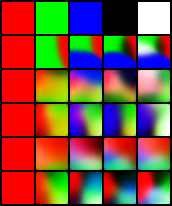
Figure 8: CompVAE, 2D problem. First row: parts $\ell_{\_}1\ldots\ell_{\_}5$. Second row: the $i$-th square depicts the $x$ defined from $\ell_{\_}1$ to $\ell_{\_}i$ as generated by the ground truth. Rows 3-6: different realizations of the same combination by the trained CompVAE - see text. Best viewed in colors.

6 Discussion and Perspectives

The main contribution of the paper is the generative framework CompVAE, to our best knowledge the first generative framework able to support the generation of data based on a multi-ensemble $\{\ell_{\_}i\}$. Built on the top of the celebrated VAE, CompVAE learns to optimize the conditional distribution $p_{\_}\theta(x|\{\ell_{\_}i\})$ in a theoretically sound way, through introducing latent variables (one for each part $\ell_{\_}i$), enforcing their order-invariant aggregation and learning another latent variable to model the interaction of the parts. Two proofs of concepts for the approach, respectively concerning a 1D and a 2D problem, have been established with respectively very satisfactory and satisfactory results.

This work opens several perspectives for further research. A first direction in the domain of computer vision consists of combining CompVAE with more advanced image generation models such as PixelCNN [33] in a way similar to PixelVAE [11], in order to generate realistic images involving a predefined set of elements along a consistent layout.

A second perspective is to make one step further toward the training of fully programmable generative models. The idea is to incorporate explicit biases on the top of the distribution learned from unbiased data, to be able to sample the desired sub-spaces of the data space. In the motivating application domain of electric consumption for instance, one would like to sample the global consumption curves associated with high consumption peaks, that is, to bias the generation process toward the top quantiles of the overall distribution.

Appendix A Model structures

Appendix B Data generation

Appendix C Multivariate Gaussian parametrization

References

- [1] Alessandro Achille and Stefano Soatto. Emergence of invariance and disentanglement in deep representations. The Journal of Machine Learning Research, 19(1):1947–1980, 2018.
- [2] Yoshua Bengio, Aaron Courville, and Pascal Vincent. Representation learning: A review and new perspectives. IEEE Transactions on Pattern Analysis and Machine Intelligence, 35(8):1798–1828, 2013.
- [3] Xi Chen, Yan Duan, Rein Houthooft, John Schulman, Ilya Sutskever, and Pieter Abbeel. Infogan: Interpretable representation learning by information maximizing generative adversarial nets. In Advances in neural information processing systems, pages 2172–2180, 2016.
- [4] Jan Chorowski, Ron J. Weiss, Samy Bengio, and Aäron van den Oord. Unsupervised speech representation learning using WaveNet autoencoders. url: http://arxiv.org/abs/1901.08810, 2019.
- [5] Junyoung Chung, Kyle Kastner, Laurent Dinh, Kratarth Goel, Aaron C Courville, and Yoshua Bengio. A recurrent latent variable model for sequential data. In C. Cortes, N. D. Lawrence, D. D. Lee, M. Sugiyama, and R. Garnett, editors, Advances in Neural Information Processing Systems 28, pages 2980–2988. 2015.
- [6] John D. Co-Reyes, YuXuan Liu, Abhishek Gupta, Benjamin Eysenbach, Pieter Abbeel, and Sergey Levine. Self-consistent trajectory autoencoder: Hierarchical reinforcement learning with trajectory embeddings. International Conference on Machine Learning, 2018.
- [7] Vincent Dumoulin, Ishmael Belghazi, Ben Poole, Olivier Mastropietro, Alex Lamb, Martin Arjovsky, and Aaron Courville. Adversarially learned inference. International Conference on Learning Representations, 2017.
- [8] Justin Gilmer, Samuel S. Schoenholz, Patrick F. Riley, Oriol Vinyals, and George E. Dahl. Neural message passing for quantum chemistry. In International Conference on Machine Learning, pages 1263–1272, 2017.
- [9] Ian Goodfellow, Jean Pouget-Abadie, Mehdi Mirza, Bing Xu, David Warde-Farley, Sherjil Ozair, Aaron Courville, and Yoshua Bengio. Generative adversarial nets. In Advances in Neural Information Processing Systems 27, pages 2672–2680. Curran Associates, Inc., 2014.
- [10] Arthur Gretton, Karsten M. Borgwardt, Malte J. Rasch, Bernhard Schölkopf, and Alexander Smola. A kernel two-sample test. The Journal of Machine Learning Research, 13:723–773, 2012.
- [11] Ishaan Gulrajani, Kundan Kumar, Faruk Ahmed, Adrien Ali Taiga, Francesco Visin, David Vazquez, and Aaron Courville. PixelVAE: A latent variable model for natural images. International Conference on Learning Representations, 2017.
- [12] Irina Higgins, Loic Matthey, Arka Pal, Christopher Burgess, Xavier Glorot, Matthew Botvinick, Shakir Mohamed, and Alexander Lerchner. beta-VAE: Learning basic visual concepts with a constrained variational framework. International Conference on Learning Representations, 2017.
- [13] Wei-Ning Hsu, Yu Zhang, and James Glass. Unsupervised learning of disentangled and interpretable representations from sequential data. In Advances in Neural Information Processing Systems 30, pages 1878–1889. Curran Associates, Inc., 2017.
- [14] Michael I. Jordan, Zoubin Ghahramani, Tommi S. Jaakkola, and Lawrence K. Saul. An introduction to variational methods for graphical models. Machine Learning, 37(2):183–233, 1999.
- [15] Diederik P. Kingma and Jimmy Ba. Adam: A method for stochastic optimization. International Conference on Learning Representations, 2014.
- [16] Diederik P. Kingma, Danilo J. Rezende, Shakir Mohamed, and Max Welling. Semi-supervised learning with deep generative models. Neural Information Processing Systems, 2014.
- [17] Diederik P. Kingma and Max Welling. Auto-encoding variational bayes. International Conference on Learning Representations, 2013.
- [18] Tejas D Kulkarni, William F. Whitney, Pushmeet Kohli, and Josh Tenenbaum. Deep convolutional inverse graphics network. In Advances in Neural Information Processing Systems 28, pages 2539–2547. Curran Associates, Inc., 2015.
- [19] Abhishek Kumar, Prasanna Sattigeri, and Avinash Balakrishnan. Variational inference of disentangled latent concepts from unlabeled observations. International Conference on Learning Representations, 2017.
- [20] Li Liu, Wanli Ouyang, Xiaogang Wang, Paul Fieguth, Jie Chen, Xinwang Liu, and Matti Pietikäinen. Deep learning for generic object detection: A survey. url: http://arxiv.org/abs/1809.02165, 2018.
- [21] Christos Louizos, Kevin Swersky, Yujia Li, Max Welling, and Richard Zemel. The variational fair autoencoder. url: http://arxiv.org/abs/1511.00830, 2015.
- [22] Lars Maaløe, Casper Kaae Sønderby, Søren Kaae Sønderby, and Ole Winther. Auxiliary deep generative models. In International Conference on Machine Learning, pages 1445–1453, 2016.
- [23] Mehdi Mirza and Simon Osindero. Conditional generative adversarial nets. url: http://arxiv.org/abs/1411.1784, 2014.
- [24] Daniel Moyer, Shuyang Gao, Rob Brekelmans, Aram Galstyan, and Greg Ver Steeg. Invariant representations without adversarial training. In Advances in Neural Information Processing Systems, pages 9084–9093, 2018.
- [25] Dilip K Prasad. Survey of the problem of object detection in real images. International Journal of Image Processing (IJIP), 6(6):441, 2012.
- [26] Alec Radford, Luke Metz, and Soumith Chintala. Unsupervised representation learning with deep convolutional generative adversarial networks. International Conference on Learning Representations, 2015.
- [27] Danilo Jimenez Rezende, Shakir Mohamed, and Daan Wierstra. Stochastic backpropagation and approximate inference in deep generative models. In International Conference on Machine Learning, pages 1278–1286, 2014.
- [28] F. Scarselli, M. Gori, A. C. Tsoi, M. Hagenbuchner, and G. Monfardini. The graph neural network model. IEEE Transactions on Neural Networks, 20(1):61–80, 2009.
- [29] Ravid Shwartz-Ziv and Naftali Tishby. Opening the black box of deep neural networks via information. url: http://arxiv.org/abs/1703.00810, 2017.
- [30] Casper Kaae Sønderby, Tapani Raiko, Lars Maaløe, Søren Kaae Sønderby, and Ole Winther. Ladder variational autoencoders. Advances in Neural Information Processing Systems, pages 3738–3746, 2016.
- [31] Naftali Tishby, Fernando C. Pereira, and William Bialek. The information bottleneck method. CoRR, physics/0004057, 2000.
- [32] Luan Tran, Xi Yin, and Xiaoming Liu. Disentangled representation learning GAN for pose-invariant face recognition. In Proceedings of the IEEE Conference on Computer Vision and Pattern Recognition, pages 1415–1424, 2017.
- [33] Aaron van den Oord, Nal Kalchbrenner, Lasse Espeholt, koray kavukcuoglu koray, Oriol Vinyals, and Alex Graves. Conditional image generation with PixelCNN decoders. In Advances in Neural Information Processing Systems 29, pages 4790–4798. Curran Associates, Inc., 2016.
- [34] Stefan Webb, Adam Golinski, Rob Zinkov, Siddharth Narayanaswamy, Tom Rainforth, Yee Whye Teh, and Frank Wood. Faithful inversion of generative models for effective amortized inference. In Advances in Neural Information Processing Systems, pages 3070–3080, 2018.
- [35] Rich Zemel, Yu Wu, Kevin Swersky, Toni Pitassi, and Cynthia Dwork. Learning fair representations. In International Conference on Machine Learning, pages 325–333, 2013.