Superconductivity by Hidden Spin Fluctuations in Electron-Doped Iron Selenide

Abstract

Berg, Metlitski and Sachdev, Science 338, 1606 (2012), have shown that the exchange of hidden spin fluctuations by conduction electrons with two orbitals can result in high-temperature superconductivity in copper-oxide materials. We introduce a similar model for high-temperature iron-selenide superconductors that are electron doped. Conduction electrons carry the minimal $3d_{xz}$ and $3d_{yz}$ iron-atom orbitals. Low-energy hidden spin fluctuations at the checkerboard wavevector ${\bm{Q}}_{\rm AF}$ result from nested Fermi surfaces at the center and at the corner of the unfolded (one-iron) Brillouin zone. Magnetic frustration from super-exchange interactions via the selenium atoms stabilize hidden spin fluctuations at ${\bm{Q}}_{\rm AF}$ versus true spin fluctuations. At half filling, Eliashberg theory based purely on the exchange of hidden spin fluctuations reveals a Lifshitz transition to electron/hole Fermi surface pockets at the corner of the folded (two-iron) Brillouin zone, but with vanishing spectral weights. The underlying hidden spin-density wave groundstate is therefore a Mott insulator. Upon electron doping, Eliashberg theory finds that the spectral weights of the hole Fermi surface pockets remain vanishingly small, while the spectral weights of the larger electron Fermi surface pockets become appreciable. This prediction is therefore consistent with the observation of electron Fermi surface pockets alone in electron-doped iron selenide by angle-resolved photoemission spectroscopy (ARPES). Eliashberg theory also finds an instability to $S^{+-}$ superconductivity at electron doping, with isotropic Cooper pairs that alternate in sign between the visible electron Fermi surface pockets and the faint hole Fermi surface pockets. Comparison with the isotropic energy gaps observed in electron-doped iron selenide by ARPES and by scanning tunneling microscopy (STM) is consistent with short-range hidden magnetic order.

I Introduction

Electron-doped iron selenides are perhaps the most interesting class of materials inside the family of iron-based superconductorsqian_11 ; xu_12 ; zheng_11 ; yu_11 . By contrast with bulk FeSe, which is a low-temperature superconductor, a monolayer of FeSe on a doped strontium-titanate substrate becomes a high-temperature superconductorxue_12 , with a critical temperature in the range $40$-$50$ Kzhang_14 ; deng_14 , and possibly higherge_15 . Angle-resolved photoemission spectroscopy (ARPES) reveals that the substrate injects electrons into the FeSe monolayer that bury the hole bands at the center of the Brillouin zone below the Fermi levelliu_12 . ARPES also reveals an energy gap at the remaining electron-type Fermi surface pockets at the corner of the folded (two-iron) Brillouin zonepeng_14 ; lee_14 . It agrees with the energy gap found by scanning tunneling microscopy (STM)xue_12 ; fan_15 . On the other hand, transport studies find perfect conductivity below the critical temperature where the gap opens in ARPES and in STMzhang_14 ; ge_15 . These probes provide compelling evidence for a superconducting state at high temperature. Electron doping of FeSe layers can also be achieved by other means, such as by alkali-atom intercalationqian_11 ; xu_12 ; zheng_11 ; yu_11 , and by organic-molecule intercalationzhao_16 ; niu_15 ; yan_15 . These systems show the same Lifshitz transition of the Fermi surface topology, where the hole bands are buried below the Fermi level at the $\Gamma$-point, but where electron Fermi surface pockets at the corner of the folded Brillouin zone remain. These systems also show high-temperature superconductivity, with an isotropic energy gap that opens at the electron-type Fermi surface pockets.

The coincidence of high-temperature superconductivity with the absence of Fermi surface nesting in electron-doped FeSe is puzzling. High-temperature superconductivity in iron-pnictide materials occurs only when the Fermi surfaces exhibit partial nesting, for example. In particular, the end-member compound KFe₂As₂ of the series of iron-pnictide compoundsbudko_prb_13 (Ba_1-xK_x)Fe₂As₂ shows hole-type Fermi surface pockets at the center of the Brillouin zone, but no electron Fermi surface pockets at the corner of the folded Brillouin zone to nest withsato_prl_09 . It is a low-temperature superconductor with $T_{c}\cong 3$ K, however. Early theoretical responses to the puzzle posed by electron-doped iron selenide proposed a nodeless $D$-wave superconducting statemaier_11 ; wang_11 , with a full gap over each electron pocket that alternates in sign between them. In the case of bulk electron-doped iron-selenide materials, it was argued that strong dispersion of the energy bands along the $c$ axis results in inner and outer electron Fermi surface pockets at the corner of the folded Brillouin zone because of hybridization due to the two inequivalent iron sites, and that true $D$-wave nodes appear as a resultmazin_11 . In the case of an isolated layer of FeSe, the two electron Fermi surface pockets at the corner of the two-iron Brillouin zone cross, but do not hybridize, because of glide-reflection symmetryLee_Wen_08 . Inner and outer electron Fermi surface pockets due to hybridization are predicted when strong enough spin-orbit coupling is included, however, and true $D$-wave nodes are again predictedagterberg_17 ; eugenio_vafek_18 . These considerations led to the proposal of the anti-bonding $S^{+-}$ state. It is an isotropic Cooper pair state that alternates in sign between the inner and the outer electron Fermi surfaces at the corner of the folded (two-iron) Brillouin zone mazin_11 ; khodas_chubukov_12 . ARPES finds no sign of nodes in the gap and no sign of hybridization on the electron Fermi surface pocketspeng_14 ; lee_14 , however. Further, STM and the dependence of the specific heat and of nuclear magnetic resonance (NMR) on temperature are consistent with a gap over the entire Fermi surfacezheng_11 ; yu_11 ; xue_12 . These measurements could then rule out the nodeless $D$-wave state and the anti-bonding $S^{+-}$ state in high-$T_{c}$ iron-selenide superconductors.

Below, we will show that a spin-fermion model over the square lattice that is similar to that introduced by Berg, Metlitski and Sachdev in the context of copper-oxide high-temperature superconductorsBMS_12 harbors an alternative solution to the puzzling isotropic gap shown by electron-doped iron selenide. The non-interacting electrons are in the principal $3d_{xz}$ and $3d_{yz}$ iron orbitals, and they form a semi-metallic Fermi surface that is nested by the checkerboard wavevector ${\bm{Q}}_{\rm AF}=(\pi/a,\pi/a)$. The latter can result in hidden magnetic order when magnetic frustration is present, at weak enough Hund’s Rule couplingjpr_rm_18 . Such hidden antiferromagnetism is characterized by the most symmetric of three possible order parameters for a hidden spin density wave (hSDW):

$${1\over{2{\cal N}}}\sum_{i}e^{i{\bm{Q}}_{\rm AF}\cdot{\bm{r}}_{i}}\sum_{s=\uparrow,\downarrow}({\rm sgn}\,s)i\langle c_{i,d_{xz},s}^{\dagger}c_{i,d_{yz},s}-c_{i,d_{yz},s}^{\dagger}c_{i,d_{xz},s}\rangle,$$

where ${\cal N}$ is the number of site-orbitals. It is isotropic with respect to rotations of the orbitals about the $z$ axis, and it therefore does not couple to nematicity. (Cf. refs. xu_muller_sachdev_08 ; kang_fernandez_16 .) Based on the interaction of such fermions with the corresponding hidden spin fluctuations, an Eliashberg theory for $S$-wave pairing over the two bands of electrons is developed. Hopping matrix elements are chosen so that perfect nesting exists at half fillingjpr_rm_18 . As the interaction grows strong, we find (i) a Lifshitz transition to electron-type and hole-type Fermi surface pockets at the corner of the folded (two-iron) Brillouin zone. The new Fermi surfaces remain perfectly nested by ${\bm{Q}}_{\rm AF}$, but their spectral weights are vanishingly small due to strong wavefunction renormalization. Upon electron doping, the hole Fermi surfaces remain faint, while the electron Fermi surfaces become visible because of only moderate wavefunction renormalization. This prediction agrees with previous calculations based on the corresponding local-moment modeljpr_17 . The Eliashberg theory also reveals (ii) an instability at the renormalized Fermi surface to $S^{+-}$ pairing that alternates in sign between the visible electron-type Fermi surfaces and the faint hole-type Fermi surfaces. We shall now provide details of how such hidden $S^{+-}$ superconductivity emerges from the two-band Eliashberg theory.

II Bare Nested Fermi Surfaces and Hidden Spin Fluctuations

The conditions for perfect nesting of the Fermi surfaces in two-orbital hopping Hamiltonians for iron selenide will be determined in what followsjpr_rm_18 . Also, the space of hSWD states generated by rotations of the two isospin degrees of freedom, the $d+$ and $d-$ orbitals, will be discussed.

II.1 Electron Hopping

The electronic kinetic energy is governed by the hopping Hamiltonian

$$H_{\rm hop}=-\sum_{\langle i,j\rangle}(t_{1}^{\alpha,\beta}c_{i,\alpha,s}^{\dagger}c_{j,\beta,s}+{\rm h.c.})-\sum_{\langle\langle i,j\rangle\rangle}(t_{2}^{\alpha,\beta}c_{i,\alpha,s}^{\dagger}c_{j,\beta,s}+{\rm h.c.}),$$ (1)

where the repeated indices $\alpha$ and $\beta$ are summed over the iron ${d+}$ and ${d-}$ orbitals, where the repeated index $s$ is summed over electron spin, and where $\langle i,j\rangle$ and $\langle\langle i,j\rangle\rangle$ represent nearest neighbor (1) and next-nearest neighbor (2) links on the square lattice of iron atoms. Above, $c_{i,\alpha,s}$ and $c_{i,\alpha,s}^{\dagger}$ denote annihilation and creation operators for an electron of spin $s$ in orbital $\alpha$ at site $i$. We keep only the $3d_{xz}$ and $3d_{yz}$ orbitals of the iron atoms, which are the principal ones in iron selenide. In particular, let us work in the isotropic basis of orbitals $d-=(d_{xz}-id_{yz})/{\sqrt{2}}$ and $d+=(d_{xz}+id_{yz})/{\sqrt{2}}$. The reflection symmetries shown by a single layer of iron selenide imply that the above intra-orbital and inter-orbital hopping matrix elements show $s$-wave and $d$-wave symmetry, respectivelyLee_Wen_08 ; raghu_08 ; jpr_mana_pds_14 . In particular, nearest neighbor hopping matrix elements satisfy

$$t_{1}^{\pm\pm}({\hat{\bm{x}}}) = t_{1}^{\parallel}=t_{1}^{\pm\pm}({\hat{\bm{y}}})$$

$$t_{1}^{\pm\mp}({\hat{\bm{x}}}) = t_{1}^{\perp}=-t_{1}^{\pm\mp}({\hat{\bm{y}}}),$$ (2)

where $t_{1}^{\parallel}$ and $t_{1}^{\perp}$ are real, while next-nearest neighbor hopping matrix elements satisfy

$$t_{2}^{\pm\pm}({\hat{\bm{x}}}+{\hat{\bm{y}}})=\;t_{2}^{\parallel} = t_{2}^{\pm\pm}({\hat{\bm{y}}}-{\hat{\bm{x}}})$$

$$t_{2}^{\pm\mp}({\hat{\bm{x}}}+{\hat{\bm{y}}})=\pm t_{2}^{\perp} = -t_{2}^{\pm\mp}({\hat{\bm{y}}}-{\hat{\bm{x}}}),$$ (3)

where $t_{2}^{\parallel}$ is real, and where $t_{2}^{\perp}$ is pure imaginary.

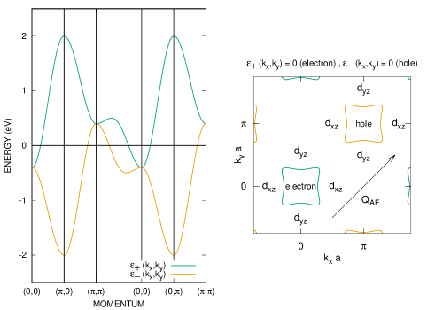
Figure 1: Band structure with perfectly nested Fermi surfaces at half filling: $\varepsilon_{+}({\bm{k}})=0$ and $\varepsilon_{-}({\bm{k}})=0$, with hopping matrix elements $t_{1}^{\parallel}=100$ meV, $t_{1}^{\perp}=500$ meV, $t_{2}^{\parallel}=0$, and $t_{2}^{\perp}/i=100$ meV.

The above hopping Hamiltonian $H_{\rm hop}$ then has intra-orbital and inter-orbital matrix elements

$$\varepsilon_{\parallel}({\bm{k}})= -2t_{1}^{\parallel}(\cos k_{x}a+\cos k_{y}a)-2t_{2}^{\parallel}(\cos k_{+}a+\cos k_{-}a)$$ (4a)

$$\varepsilon_{\perp}({\bm{k}})= -2t_{1}^{\perp}(\cos k_{x}a-\cos k_{y}a)-2t_{2}^{\perp}(\cos k_{+}a-\cos k_{-}a)$$ (4b)

with $k_{\pm}=k_{x}\pm k_{y}$. It is easily diagonalized by plane waves of $d_{x(\delta)z}$ and $id_{y(\delta)z}$ orbitals that are rotated with respect to the principal axes by an angle $\delta({\bm{k}})$:

$$|{\bm{k}},d_{x(\delta)z}\rangle\rangle = {\cal N}^{-1/2}\sum_{i}e^{i{\bm{k}}\cdot{\bm{r}}_{i}}[e^{i\delta({\bm{k}})}|i,d+\rangle+e^{-i\delta({\bm{k}})}|i,d-\rangle],$$

$$i|{\bm{k}},d_{y(\delta)z}\rangle\rangle = {\cal N}^{-1/2}\sum_{i}e^{i{\bm{k}}\cdot{\bm{r}}_{i}}[e^{i\delta({\bm{k}})}|i,d+\rangle-e^{-i\delta({\bm{k}})}|i,d-\rangle],$$ (5)

where ${\cal N}=2N_{\rm Fe}$ is the number of iron site-orbitals. The phase shift $\delta({\bm{k}})$ is set by $\varepsilon_{\perp}({\bm{k}})=|\varepsilon_{\perp}({\bm{k}})|e^{i2\delta({\bm{k}})}$. Specifically,

$$\cos\,2\delta({\bm{k}})= {-t_{1}^{\perp}(\cos\,k_{x}a-\cos\,k_{y}a)\over{\sqrt{t_{1}^{\perp 2}(\cos\,k_{x}a-\cos\,k_{y}a)^{2}+|2t_{2}^{\perp}|^{2}(\sin\,k_{x}a)^{2}(\sin\,k_{y}a)^{2}}}},$$ (6a)

$$\sin\,2\delta({\bm{k}})= {2(t_{2}^{\perp}/i)(\sin\,k_{x}a)(\sin\,k_{y}a)\over{\sqrt{t_{1}^{\perp 2}(\cos\,k_{x}a-\cos\,k_{y}a)^{2}+|2t_{2}^{\perp}|^{2}(\sin\,k_{x}a)^{2}(\sin\,k_{y}a)^{2}}}}.$$ (6b)

The phase shift is notably singular at ${\bm{k}}=0$ and ${\bm{Q}}_{\rm AF}=(\pi/a,\pi/a)$, where the matrix element $\varepsilon_{\perp}({\bm{k}})$ vanishes. The energy eigenvalues of the bonding ($+$) and anti-bonding ($-$) plane waves (5) are respectively given by $\varepsilon_{+}({\bm{k}})=\varepsilon_{\parallel}({\bm{k}})+|\varepsilon_{\perp}({\bm{k}})|$ and $\varepsilon_{-}({\bm{k}})=\varepsilon_{\parallel}({\bm{k}})-|\varepsilon_{\perp}({\bm{k}})|$.

Henceforth, we shall turn off next-nearest neighbor intra-orbital hopping: $t_{2}^{\parallel}=0$. Notice that the above energy bands now satisfy the perfect nesting condition

$$\varepsilon_{\pm}({\bm{k}}+{\bm{Q}}_{\rm AF})=-\varepsilon_{\mp}({\bm{k}}),$$ (7)

where ${\bm{Q}}_{\rm AF}=(\pi/a,\pi/a)$ is the wavevector for the checkerboard on the square lattice of iron atoms. The Fermi level at half filling therefore lies at $\epsilon_{\rm F}=0$. Figure 1 displays perfectly nested electron-type and hole-type Fermi surfaces for hopping parameters $t_{1}^{\parallel}=100$ meV, $t_{1}^{\perp}=500$ meV, $t_{2}^{\parallel}=0$ and $t_{2}^{\perp}/i=100$ meV. Figure 2 shows the density of states of the bonding ($+$) band.

Figure 2: Density of states of the bonding band evaluated numerically at hopping parameters that are listed in the caption to Fig. 1: $a^{2}D_{+}(\varepsilon)=N_{\rm Fe}^{-1}\sum_{\bm{k}}\delta[\varepsilon-\varepsilon_{+}({\bm{k}})]$. The unfolded (one-iron) Brillouin zone is divided into a $10,000\times 10,000$ grid, while the $\delta$-function is approximated by $(4k_{B}T_{0})^{-1}{\rm sech}^{2}(\varepsilon/2k_{B}T_{0})$. Here, $k_{B}T_{0}$ is $3$ parts in $10,000$ of the bandwidth.

II.2 Extended Hubbard Model

The Hamiltonian of the underlying extended Hubbard modeljpr_rm_18 has three parts: $H=H_{\rm hop}+H_{U}+H_{\rm sprx}$. On-site Coulomb repulsion is counted by the second term2orb_Hbbrd ,

$$H_{U}=\sum_{i} [U_{0}n_{i,\alpha,\uparrow}n_{i,\alpha,\downarrow}+J_{0}{\bm{S}}_{i,d-}\cdot{\bm{S}}_{i,d+}$$ (8)

$$+U_{0}^{\prime}n_{i,d+}n_{i,d-}+J_{0}^{\prime}(c_{i,d+,\uparrow}^{\dagger}c_{i,d+,\downarrow}^{\dagger}c_{i,d-,\downarrow}c_{i,d-,\uparrow}+{\rm h.c.})].$$

where $n_{i,\alpha,s}$ is the occupation operator, and where $n_{i,\alpha}=n_{i,\alpha,\uparrow}+n_{i,\alpha,\downarrow}$. Also, ${\bm{S}}_{i,\alpha}$ is the spin operator. Above, $U_{0}>0$ is the intra-orbital on-site Coulomb repulsion energy, while $U_{0}^{\prime}>0$ is the inter-orbital one. It is worth pointing out the following expression for the sum of these two on-site repulsion terms in (8):

$$U_{0}n_{i,\alpha,\uparrow}n_{i,\alpha,\downarrow}+U_{0}^{\prime}n_{i,d+}n_{i,d-}=(U_{0}-U_{0}^{\prime})n_{i,\alpha,\uparrow}n_{i,\alpha,\downarrow}+{1\over 2}U_{0}^{\prime}\,n_{i}(n_{i}-1),$$ (9)

where $n_{i}=n_{i,d+}+n_{i,d-}$ is the net occupation per iron site $i$. Above also, $J_{0}$ is the Hund’s Rule exchange coupling constant, which has a ferromagnetic (negative) sign, while $J_{0}^{\prime}$ is the matrix element for on-site Josephson tunneling between orbitals. The third and last term in the Hamiltonian represents super-exchange interactions among the iron spins via the selenium atoms:

$$H_{\rm sprx}=\sum_{\langle i,j\rangle} J_{1}^{({\rm sprx})}({\bm{S}}_{i,d-}+{\bm{S}}_{i,d+})\cdot({\bm{S}}_{j,d-}+{\bm{S}}_{j,d+})$$ (10)

$$+\sum_{\langle\langle i,j\rangle\rangle}J_{2}^{({\rm sprx})}({\bm{S}}_{i,d-}+{\bm{S}}_{i,d+})\cdot({\bm{S}}_{j,d-}+{\bm{S}}_{j,d+}).$$

Above, $J_{1}^{({\rm sprx})}$ and $J_{2}^{({\rm sprx})}$ are positive super-exchange coupling constants over nearest neighbor and next-nearest neighbor iron sites.

$I^{(3)}$ $|$ $S^{(z)}/\hbar$	isospin triplet ($I=1$), spin singlet ($S=0$)	isospin singlet ($I=0$), spin triplet ($S=1$)
$+1$	${d+}_{1}{d+}_{2}{1\over{\sqrt{2}}}(\uparrow_{1}\downarrow_{2}-\downarrow_{1}\uparrow_{2})$	${1\over{\sqrt{2}}}({d+}_{1}{d-}_{2}-{d-}_{1}{d+}_{2})\uparrow_{1}\uparrow_{2}$
$0$	${1\over{\sqrt{2}}}({d+}_{1}{d-}_{2}+{d-}_{1}{d+}_{2}){1\over{\sqrt{2}}}(\uparrow_{1}\downarrow_{2}-\downarrow_{1}\uparrow_{2})$	${1\over{\sqrt{2}}}({d+}_{1}{d-}_{2}-{d-}_{1}d+_{2}){1\over{\sqrt{2}}}(\uparrow_{1}\downarrow_{2}+\downarrow_{1}\uparrow_{2})$
$-1$	${d-}_{1}{d-}_{2}{1\over{\sqrt{2}}}(\uparrow_{1}\downarrow_{2}-\downarrow_{1}\uparrow_{2})$	${1\over{\sqrt{2}}}({d+}_{1}{d-}_{2}-{d-}_{1}{d+}_{2})\downarrow_{1}\downarrow_{2}$

Table 1: Atomic iron states at half filling. The isospin triplet states violate Hund’s Rule, while the isospin singlet states obey Hund’s Rule.

It is instructive to uncover the energy spectrum of the Hamiltonian $H_{U}$ at a single iron site $i$, at half filling with two electrons. Table 1 gives the corresponding six-dimensional Hilbert space in the singlet-triplet/spin-isospin basis. Here, the $d+$ and the $d-$ orbitals comprise the isospin-1/2 states. Specifically, the isospin operators along the axes $n=1,2,3$ for a single electron have the form $I^{(n)}=+{1\over 2}|u_{n}\rangle\langle u_{n}|-{1\over 2}|v_{n}\rangle\langle v_{n}|$, with orbitals $(u_{1},v_{1})=(d_{xz},d_{yz})$, $(u_{2},v_{2})=(d_{x^{\prime}z},d_{y^{\prime}z})$, and $(u_{3},v_{3})=({d+},{d-})$. Here, $x^{\prime}=(x+y)/\sqrt{2}$ and $y^{\prime}=(-x+y)/\sqrt{2}$. The eigenstates of (8) at a single iron site are the product of spin ($S=1$) triplet states with the isospin ($I=0$) singlet state

$$\phi_{0}(1,2)={1\over{\sqrt{2}}}[u_{n}(1)v_{n}(2)-v_{n}(1)u_{n}(2)],$$ (11)

and the product of the spin ($S=0$) singlet state with the isospin ($I=1$) triplet states

$$\phi_{n}(1,2)={1\over{\sqrt{2}}}[u_{n}(1)v_{n}(2)+v_{n}(1)u_{n}(2)],\quad n=1,2,3.$$ (12)

Recall that the isospin singlet pair state $\phi_{0}(1,2)$ is unique up to a phase factor. The orbital pair states (11) and (12) above satisfy $I^{(n)}\phi_{0}=0$ and $I^{(n)}\phi_{n}=0$, where $I^{(n)}=I^{(n)}(1)+I^{(n)}(2)$. And why do the pair states (11) and (12) make up the energy spectrum of $H_{U}$? First, observe that the spin singlet and spin triplet states listed in Table 1 are all eigenstates of the Hund’s Rule term in (8), with energy splitting $E^{(0)}_{\rm singlet}-E^{(0)}_{\rm triplet}=-J_{0}$. Second, notice that all six pair states listed in Table 1 are eigenstates of the sum (9) of the intra-orbital and inter-orbital on-site repulsion terms in (8), with energy splitting between the doubly occupied and singly occupied $d+$ and $d-$ orbitals, $E^{(0)}_{d(1)d(2)}-E^{(0)}_{d(1){\bar{d}}(2)}=U_{0}-U_{0}^{\prime}$. Third, notice that the pair states $\phi_{1}(1,2)$ and $\phi_{2}(1,2)$ are odd and even superpositions of ${d+}(1){d+}(2)$ and ${d-}(1){d-}(2)$. The former pair states, hence, are eigenstates of the on-site Josephson tunneling terms in (8), with energy splitting $E^{(0)}_{1}-E^{(0)}_{2}=-2J_{0}^{\prime}$. The remaining pair states $\phi_{0}(1,2)$ and $\phi_{3}(1,2)$ do not participate in on-site Josephson tunneling. Table 2 lists the atomic energies of these pair states compared to the one along the isospin $I^{(3)}$ axis.

Isospin Axis of Pair State $(n)$	$S$	$I$	$\Delta H_{U}$
any $(0)$	$1$	$0$	$J_{0}$
$I^{(1)}$	$0$	$1$	$U_{0}-U_{0}^{\prime}-J_{0}^{\prime}$
$I^{(2)}$	$0$	$1$	$U_{0}-U_{0}^{\prime}+J_{0}^{\prime}$
$I^{(3)}$	$0$	$1$	$0$

Table 2: Relative energy $H_{U}$ of atomic pair states, $\phi_{n}(1,2)$, compared to that of $\phi_{3}(1,2)$. Recall that $J_{0}<0$.

Last, we point out that both the on-site Josephson tunneling terms in (8) and the first term in (9) for the on-site repulsion break isospin rotation invariance. Such symmetry-breaking contributions in the on-site Hamiltonian $H_{U}$ are consolidated by the Hamiltonian

$$H_{U}^{\prime}=\sum_{i}2[+J_{0}^{\prime}\,I_{i,\uparrow}^{(1)}I_{i,\downarrow}^{(1)}-J_{0}^{\prime}\,I_{i,\uparrow}^{(2)}I_{i,\downarrow}^{(2)}+(U_{0}-U_{0}^{\prime})I_{i,\uparrow}^{(3)}I_{i,\downarrow}^{(3)}],$$ (13)

where ${\bm{I}}_{i,\uparrow}$ and ${\bm{I}}_{i,\downarrow}$ are the respective isospin operators for spin-$\uparrow$ and spin-$\downarrow$ electrons at iron site $i$. (See Appendix A.) They each represent $2\times 2$ isospin operators acting on the $d+$ and $d-$ orbitals for an electron of such spin.

II.3 Hidden Magnetic Order

The true electronic spin at an iron site $i$ is measured by the operator ${\bm{S}}_{i}={\bm{S}}_{i,d+}+{\bm{S}}_{i,d-}$, with ${\bm{S}}_{i,\alpha}=({\hbar}/2)\sum_{s,s^{\prime}}c_{i,\alpha,s}^{\dagger}{\bm{\sigma}}_{s,s^{\prime}}c_{i,\alpha,s^{\prime}}$, where ${\bm{\sigma}}$ denote the Pauli matrices. In the present case, we keep only the principal $d-$ and $d+$ orbitals, $\alpha$. Hidden spin excitations must be orthogonal to true spin excitations. Hidden spin excitations then correspond to “pion” excitations of the latter isospin degrees of freedom. Table 3 lists these spin excitations explicitly, which carry isospin $I=1$. They are isospin components of the tensor product $({\bm{S}}\otimes{\bm{I}})_{i}=(\hbar/4)\sum_{\alpha,\alpha^{\prime}}\sum_{s,s^{\prime}}c_{i,\alpha,s}^{\dagger}{\bm{\sigma}}_{s,s^{\prime}}{\bm{\tau}}_{\alpha,\alpha^{\prime}}c_{i,\alpha^{\prime},s^{\prime}}$, where ${\bm{\tau}}$ also denote the Pauli matrices. (See Appendix A.) Notice that hidden spin excitations generated by the ($\pi^{0}$) operator $2({\bm{S}}\otimes I^{(3)})_{i}={\bm{S}}_{i,d+}-{\bm{S}}_{i,d-}$ are the most symmetric ones, showing isotropy about the orbital $z$ axis. This is displayed explicitly by Table 4, in the row corresponding to the isospin quantization axis $I^{(3)}$, where $2({\bm{S}}\otimes I^{(3)})_{i}$ is written in terms of $d_{xz}$ and $d_{yz}$ orbitals. Figure 3 shows three different hidden spin-density orderings made up, respectively, of the three magnetic moments $2({\bm{S}}\otimes I^{(n)})_{i}$ over the square lattice $i$, with $n=1,2,3$. Such hSDW groundstates have been introduced recently in the context of copper-oxide high-$T_{c}$ superconductorsBMS_12 , of heavy fermion compoundsriseborough_12 , and of iron-selenide high-$T_{c}$ superconductorsjpr_17 ; jpr_rm_18 .

spin operator	meson analog	$\ I\$	$I^{(3)}$	type of spin
$c_{i,d+}^{\dagger}{\bm{\sigma}}\,c_{i,d+}+c_{i,d-}^{\dagger}{\bm{\sigma}}\,c_{i,d-}$	$\omega$	$0$	$0$	true
$c_{i,d+}^{\dagger}{\bm{\sigma}}\,c_{i,d+}-c_{i,d-}^{\dagger}{\bm{\sigma}}\,c_{i,d-}$	$\pi^{0}$	$1$	$0$	hidden
$c_{i,d+}^{\dagger}{\bm{\sigma}}\,c_{i,d-}$	$\pi^{+}$	$1$	$+1$	hidden
$c_{i,d-}^{\dagger}{\bm{\sigma}}\,c_{i,d+}$	$\pi^{-}$	$1$	$-1$	hidden

Table 3: List of spin-excitation operators according to isospin. Above, ${\bm{\sigma}}$ denotes the Pauli matrices for spin, and $I$ and $I^{(3)}$ denote the isospin quantum numbers. Summation over spin indices is implicit. Meson analogs are obtained by identifying the $d+$ orbital with the $u$ quark and the $d-$ orbital with the $d$ quark. See Appendix A for a definition of the isospin operator.

In the last case, perfect nesting of electron-type and hole-type Fermi surfaces exists at half filling and $t_{2}^{\parallel}=0$, which is displayed by Fig. 1. This implies an instability to a spin-density wave at the wavevector corresponding to Néel antiferromagnetic order, ${\bm{Q}}_{\rm AF}=(\pi/a,\pi/a)$. The atomic limit discussed at the end of the previous subsection becomes a useful guide to determine the relative stability of the four checkerboard spin density waves displayed by Fig. 3 in the limit of strong on-site repulsion. First, it is important to point out that the on-site pair states that compose the hSDW groundstates displayed by Figs. 3(b)-(d) can be expressed as even and odd superpositions of spin singlet and spin triplet states,

$${1\over{\sqrt{2}}}\phi_{n}(1,2){1\over{\sqrt{2}}}(\uparrow_{1}\downarrow_{2}-\downarrow_{1}\uparrow_{2})\pm{1\over{\sqrt{2}}}\phi_{0}(1,2){1\over{\sqrt{2}}}(\uparrow_{1}\downarrow_{2}+\downarrow_{1}\uparrow_{2}),$$ (14)

where $\phi_{0}(1,2)$ and $\phi_{n}(1,2)$ are orbital pair states given by (11) and (12). Such atomic pair states violate Hund’s Rule. The corresponding hSDW groundstates therefore compete with the conventional SDW groundstate displayed by Fig. 3(a) in the regime of weak Hund’s Rule coupling. Local-moment Heisenberg models find, in particular, that such hSDW states are more stable than both the conventional checkerboard and stripe SDW states in the presence of magnetic frustration (10), at weak enough Hund’s Rule couplingjpr_10 . (See Fig. 7.) And which of the three hSDW states displayed by Figs. 3(b)-(d) is the most energetically favorable one? Contrasting the corresponding atomic pair states (14) with the atomic spectrum listed by Table 2 indicates that the hSDW displayed by Fig. 3(b), which corresponds to the $I^{(3)}$ isospin axis ($n=3$), is the lowest in energy at sufficiently large intra-orbital on-site repulsion: $U_{0}-U_{0}^{\prime}>|J_{0}^{\prime}|$. Notice that both the sum of the on-site repulsion terms (9) and the on-site Josephson tunneling terms in the Hamiltonian (8) break $SU(2)$ isospin rotation invariance. These terms are collected (13) by $H_{U}^{\prime}$. Last, it is worth re-emphasizing here that the hSDW corresponding to atomic pair states (14) with $n=3$ is notably isotropic with respect to rotations of the orbitals about the $z$ axis.

hidden spin operator	isospin quantization axis	reference
$c_{i,d_{xz}}^{\dagger}{\bm{\sigma}}\,c_{i,d_{xz}}-c_{i,d_{yz}}^{\dagger}{\bm{\sigma}}\,c_{i,d_{yz}}$	$I^{(1)}$	none
$c_{i,d_{xz}}^{\dagger}{\bm{\sigma}}\,c_{i,d_{yz}}+c_{i,d_{yz}}^{\dagger}{\bm{\sigma}}\,c_{i,d_{xz}}$	$I^{(2)}$	Berg, Metlitski and Sachdev (2012)
$i(c_{i,d_{xz}}^{\dagger}{\bm{\sigma}}\,c_{i,d_{yz}}-c_{i,d_{yz}}^{\dagger}{\bm{\sigma}}\,c_{i,d_{xz}})$	$I^{(3)}$	Rodriguez (2017)

Table 4: List of hidden spin-excitation operators by isospin quantization axis. Summation over spin indices is implicit. Examples of where such hidden spin excitations appear in the literature are also listed. Note: the spin operator in the second row ($I^{(2)}$) is diagonal in the orbital basis rotated by 45 degrees about the $z$ axis; $c_{i,d_{x^{\prime}z}}^{\dagger}{\bm{\sigma}}\,c_{i,d_{x^{\prime}z}}-c_{i,d_{y^{\prime}z}}^{\dagger}{\bm{\sigma}}\,c_{i,d_{y^{\prime}z}}$, where $x^{\prime}=(x+y)/\sqrt{2}$ and $y^{\prime}=(-x+y)/\sqrt{2}$. See Appendix A for a definition of the isospin operator.

The long-range hidden Néel order shown by the hSDW state (Fig. 3b) implies low-energy spinwave excitations that collapse to zero energy at the ordering wavevector ${\bm{Q}}_{\rm AF}$. These hidden spinwaves emerge from the dynamics between the bulk spin, ${\bm{S}}_{i}={\bm{S}}_{i,d-}+{\bm{S}}_{i,d+}$, and the hidden ordered magnetic momentjpr_rm_18 , ${\bm{m}}_{i}(\pi)={\bm{S}}_{i,d-}-{\bm{S}}_{i,d+}$. It is yet another example of antiferromagnetic dynamics first discovered by Anderson anderson_52 ; halperin_hohenberg_69 ; forster_75 . The dynamical propagator for hidden spinwaves can then be defined as $iD({\bm{q}},\omega)=\langle{1\over{\sqrt{2}}}m^{+}(\pi){1\over{\sqrt{2}}}m^{-}(\pi)\rangle|_{{\bm{q}},\omega}$, where $m^{\pm}(\pi)=m_{x}(\pi)\pm i\,m_{y}(\pi)$. Here, we have assumed that the hSDW spontaneously breaks symmetry along the $z$ axis. Within the random phase approximation (RPA) of the two-orbital extended Hubbard model, recent calculations of the dynamical spin susceptibility in the hSDW state, Fig. 3b, yield the universal formhalperin_hohenberg_69 ; forster_75

$$D({\bm{q}},\omega)={(2s_{1})^{2}\over{\chi_{\perp}}}[\omega^{2}-\omega_{b}^{2}({\bm{q}})]^{-1}$$ (15)

at long wavelength and low frequencyjpr_20a . Above, $2s_{1}\hbar$ is the magnitude of the hidden ordered magnetic moment ${\bm{m}}(\pi)$ at an iron site, while $\chi_{\perp}$ is the spin susceptibility of the hSDW for external magnetic field applied perpendicular to ${\bm{m}}(\pi)$. The poles in frequency in (15) disperse as

$$\omega_{b}({\bm{q}})=(c_{b}^{2}|{\bar{\bm{q}}}|^{2}+\Delta_{b}^{2})^{1/2},$$ (16)

where ${\bm{q}}={\bar{\bm{q}}}+{\bm{Q}}_{\rm AF}$. Above, the velocity of the hidden spinwaves is given by $c_{b}=(\rho_{s}/\chi_{\perp})^{1/2}$, where $\rho_{s}$ is the spin stiffness of the hSDW, while the spin gap $\Delta_{b}$ is null when the hSDW state shows long-range order. It can be demonstrated that the spin $s_{1}$ is equal to the spin per orbital in the local-moment limit described by the two-orbital Heisenberg modeljpr_10 (74).

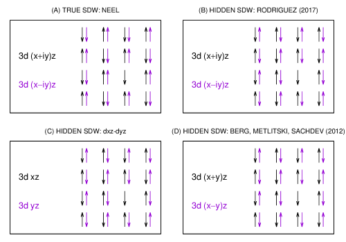
Figure 3: Spin/orbital configurations for (a) conventional Néel order, and for hidden Néel order among orbitals along (b) the $I^{(3)}$ isospin axis, along (c) the $I^{(1)}$ isospin axis, and along (d) the $I^{(2)}$ isospin axis.

III Eliashberg Theory

After adding on-iron-site Coulomb repulsion (8) and magnetic frustration from super-exchange via the selenium atoms (10) to the electron hopping Hamiltonian (1), the author and Melendrez recently showed that the hSDW state, with opposing Néel antiferromagnet order over the square lattice of iron atoms per $d\pm$ orbital, is stable within the mean-field approximation at perfect nestingjpr_rm_18 . (See Fig. 1.) And after developing an Eliashberg theory in the particle-hole channel, these authors then showed that coupling to hidden spin fluctuations, (15) and (16), shifts the two electronic bands by an equal and opposite energy, leading to electron/hole Fermi surface pockets at the corner of the folded (two-iron) Brillouin zone. They also notably found that the spectral weight, $1/Z$ , tends to zero at the new Fermi surface pockets.

Berg, Metlitski and Sachdev have performed determinant quantum Monte Carlo (DQMC) simulations on a similar modelBMS_12 that includes weak nesting of Fermi surfaces by the Néel wavevector ${\bm{Q}}_{\rm AF}$ and coupling to hidden spin fluctuations with isospin quantum number $I^{(2)}=0$. (See Table 4 and Fig. 3d.) They find a quantum-critical phase transition at low temperature between a hSDW and a $D$-wave superconductor, with Cooper pairs on nominal $x$ versus $y$ orbitals that alternate in sign between them. Below, we will show that a similar quantum-critical phase transition exists upon electron doping of the hSDW state considered here, with isospin quantum number $I^{(3)}=0$ instead. In particular, an Eliashberg theory in the conventional particle-particle channeleliashberg_60 ; eliashberg_61 ; schrieffer_64 ; scalapino_69 will be revealed for electron-doped states that exhibit only short-range hSDW order. It predicts Cooper pairs that show $S$-wave symmetry, however.

III.1 Hidden Spin Fluctuations and Interaction with Electrons

In the hidden Néel state considered here, with spontaneous symmetry breaking along the $z$ axis, the propagator for spinwaves is given by

$$\biggl{\langle}{1\over{\sqrt{2}}}m^{+}(\pi){1\over{\sqrt{2}}}m^{-}(\pi)\biggr{\rangle}\bigg{|}_{{\bm{q}},\omega}=iD({\bm{q}},\omega),$$ (17)

with its form set by (15) and (16). We shall henceforth assume that the spin gap $\Delta_{b}$ grows in a continuous fashion from zero upon crossing the quantum critical point. Electron doping from half filling shall be one of the principal tuning parameters for the quantum-critical phase transition. (Cf. Fig. 7.) Spin isotropy is recovered upon crossing the quantum critical point, however. It dictates the form

$$\biggl{\langle}{1\over{\sqrt{2}}}m^{(z)}(\pi){1\over{\sqrt{2}}}m^{(z)}(\pi)\biggr{\rangle}\bigg{|}_{{\bm{q}},\omega}={1\over 2}iD({\bm{q}},\omega),$$ (18)

for the nature of hidden spin fluctuations along the $z$ axis at $\Delta_{b}>0$.

As was mentioned earlier, the extended Hubbard model over the square lattice of iron atoms in FeSe that was introduced in subsection II.2 at perfect nesting of the Fermi surfaces (Fig. 1) harbors a hSDW state when magnetic frustration is presentjpr_rm_18 . A mean field theory approximation of the extended Hubbard model implies an isotropic interaction between spin fluctuations and electrons of the form $H_{\rm e-hsw}=-\sum_{i}\sum_{\alpha}U(\pi){\bm{m}}_{i,\alpha}\cdot 2{\bm{S}}_{i,\alpha}$, where

$$U(\pi)=U_{0}+{1\over 2}J_{0}.$$ (19)

Here, $U_{0}$ is the on-site repulsive energy cost for the formation of a spin singlet on the $d+$ orbital or on the $d-$ orbital, while $J_{0}$ is the (ferromagnetic) Hund’s Rule spin-exchange coupling constant between these two orbitals. The transverse contributions yield the interaction $H_{\rm e-hsw}^{(xy)}=-\sum_{i}\sum_{\alpha}U(\pi)(m_{i,\alpha}^{+}S_{i,\alpha}^{-}+m_{i,\alpha}^{-}S_{i,\alpha}^{+})$, while the longitudinal contributions yield the interaction $H_{\rm e-hsw}^{(z)}=-\sum_{i}\sum_{\alpha}U(\pi)m_{i,\alpha}^{(z)}2S_{i,\alpha}^{(z)}$. In the basis of electron energy bands, they yield the following contribution to the Hamiltonian due to the interaction of electrons with hidden spin fluctuations:

$$H_{\rm e-hsw}^{(xy)}=-{1\over{\sqrt{2}}}{U(\pi)\over{a{\cal N}^{1/2}}}\sum_{\bm{k}}\sum_{{\bm{k}}^{\prime}}\sum_{n}[m^{+}(\pi,{\bm{q}})c_{\downarrow}^{\dagger}({\bar{n}},{\bar{\bm{k}}}^{\prime})c_{\uparrow}(n,{\bm{k}}) {\cal M}_{n,{\bm{k}};{\bar{n}},{\bar{\bm{k}}}^{\prime}}$$ (20)

$$+{\rm h.c.}]$$

and

$$H_{\rm e-hsw}^{(z)}=-{1\over{\sqrt{2}}}{U(\pi)\over{a{\cal N}^{1/2}}}\sum_{\bm{k}}\sum_{{\bm{k}}^{\prime}}\sum_{n}\sum_{s}m^{(z)}(\pi,{\bm{q}}) c_{s}^{\dagger}({\bar{n}},{\bar{\bm{k}}}^{\prime})c_{s}(n,{\bm{k}})\cdot$$ (21)

$$\cdot{\cal M}_{n,{\bm{k}};{\bar{n}},{\bar{\bm{k}}}^{\prime}}\,({\rm sgn}\,s),$$

where ${\bm{q}}={\bm{k}}-{\bar{\bm{k}}}^{\prime}$ is the momentum transfer, with ${\bar{\bm{k}}}^{\prime}={\bm{k}}^{\prime}+{\bm{Q}}_{\rm AF}$. Above, $c_{s}^{\dagger}(n,{\bm{k}})$ and $c_{s}(n,{\bm{k}})$ are electron creation and destruction operators for plane-wave states (5). The band indices $n=1$ and $n=2$ correspond, respectively, to anti-bonding ($-$) planewaves in the $d_{y(\delta)z}$ orbital and to bonding ($+$) planewaves in the $d_{x(\delta)z}$ orbital. Also, ${\bar{n}}$ denotes the opposite band. The orbital matrix element that appears in (20) and in (21) is given byjpr_rm_18

$${\cal M}_{n,{\bm{k}};{\bar{n}},{\bar{\bm{k}}}^{\prime}}=\pm\sin[\delta({\bm{k}})+\delta({\bm{k}}^{\prime})].$$ (22)

(See Appendix B.) Above, intra-band transitions are neglected because they do not show nesting.

We shall now apply the Nambu-Gorkov formalism for paired statesschrieffer_64 ; scalapino_69 ; nambu_60 ; gorkov_58 . It then becomes useful to write the above electron-hidden-spinwave interactions in terms of spinors:

$$H_{\rm e-hsw}^{(xy)}=\mp{1\over{\sqrt{2}}}{U(\pi)\over{{a\cal N}^{1/2}}}\sum_{\bm{k}}\sum_{{\bm{k}}^{\prime}}[m^{+}(\pi,{\bm{q}})C_{n}^{\dagger}({\bar{\bm{k}}}^{\prime})\tau_{3}{\bar{C}}_{{\bar{n}}}({\bm{k}})\sin[\delta({\bm{k}}) +\delta({\bm{k}}^{\prime})]$$ (23)

$$+{\rm h.c.}],$$

and

$$H_{\rm e-hsw}^{(z)}=\mp{1\over{\sqrt{2}}}{U(\pi)\over{{a\cal N}^{1/2}}}\sum_{\bm{k}}\sum_{{\bm{k}}^{\prime}}\sum_{n}m^{(z)}(\pi,{\bm{q}}) C_{\bar{n}}^{\dagger}({\bar{\bm{k}}}^{\prime})\tau_{0}C_{n}({\bm{k}})\cdot$$ (24)

$$\cdot\sin[\delta({\bm{k}})+\delta({\bm{k}}^{\prime})],$$

with

$$C_{n}({\bm{k}})=\left[{\begin{array}[]{c}c_{\uparrow}(n,{\bm{k}})\\ c_{\downarrow}^{\dagger}(n,-{\bm{k}})\end{array}}\right]$$ (25)

and

$${\bar{C}}_{n}({\bm{k}})=\left[{\begin{array}[]{c}c_{\downarrow}(n,{\bm{k}})\\ c_{\uparrow}^{\dagger}(n,-{\bm{k}})\end{array}}\right].$$ (26)

Above, $\tau_{3}$ is the Pauli matrix along the $z$ axis, and $\tau_{0}$ is the $2\times 2$ identity matrix. Also, the explicit matrix element (22) ${\cal M}_{n,{\bm{k}};{\bar{n}},{\bar{\bm{k}}}^{\prime}}$ has been substituted in. (See Appendix B.) It is important to point out that the band index $n$ is fixed in expression (23) for $H_{\rm e-hsw}^{(xy)}$ above. The $n=1$ and the $n=2$ expressions are equivalent.

III.2 Electron Propagators and Eliashberg Equations

Let $C_{n}({\bm{k}},t)$ and ${\bar{C}}_{n}({\bm{k}},t)$ denote the time evolution of the Nambu-Gorkov spinors, $C_{n}({\bm{k}})$ and ${\bar{C}}_{n}({\bm{k}})$, and let $C_{n}^{\dagger}({\bm{k}},t)$ and ${\bar{C}}_{n}^{\dagger}({\bm{k}},t)$ denote the time evolution of their conjugates, $C_{n}^{\dagger}({\bm{k}})$ and ${\bar{C}}_{n}^{\dagger}({\bm{k}})$. The Nambu-Gorkov electron propagators are then the Fourier transforms $iG_{n}({\bm{k}},\omega)=\int dt_{1,2}e^{i\omega t_{1,2}}\langle T[C_{n}({\bm{k}},t_{1})C_{n}^{\dagger}({\bm{k}},t_{2})]\rangle$ and $i{\bar{G}}_{n}({\bm{k}},\omega)=\int dt_{1,2}e^{i\omega t_{1,2}}\langle T[{\bar{C}}_{n}({\bm{k}},t_{1}){\bar{C}}_{n}^{\dagger}({\bm{k}},t_{2})]\rangle$, where $t_{1,2}=t_{1}-t_{2}$, and where $T$ is the time-ordering operator. They are $2\times 2$ matrices. In the absence of interactions, their matrix inverses are then given by

$$G_{0n}^{-1}({\bm{k}},\omega)=\omega\,\tau_{0}-[\varepsilon_{n}({\bm{k}})-\mu_{0}]\,\tau_{3}.$$ (27)

Following the standard prescriptionschrieffer_64 ; scalapino_69 , let us next assume that the matrix inverse of the Nambu-Gorkov Greens function takes the form

$$G_{n}^{-1}({\bm{k}},\omega)=Z_{n}({\bm{k}},\omega)\omega\,\tau_{0}-[\varepsilon_{n}({\bm{k}})-\mu_{n}]\,\tau_{3}-Z_{n}({\bm{k}},\omega)\Delta_{n}({\bm{k}})\,\tau_{1}.$$ (28)

Here, $Z_{n}({\bm{k}},\omega)$ is the wavefunction renormalization, $\Delta_{n}({\bm{k}})$ is the quasi-particle gap, and $\mu_{n}-\mu_{0}$ is the shift in the energy band. Matrix inversion of (28) yields the Nambu-Gorkov Greens functionschrieffer_64 ; scalapino_69 ; nambu_60 ; gorkov_58 $G=\sum_{\mu=0}^{3}G^{(\mu)}\tau_{\mu}$, with components

$$G_{n}^{(0)} = {1\over{2Z_{n}}}\Biggl{(}{1\over{\omega-E_{n}}}+{1\over{\omega+E_{n}}}\Biggr{)},$$

$$G_{n}^{(1)} = {1\over{2Z_{n}}}\Biggl{(}{1\over{\omega-E_{n}}}-{1\over{\omega+E_{n}}}\Biggr{)}{\Delta_{n}\over E_{n}},$$

$$G_{n}^{(3)} = {1\over{2Z_{n}}}\Biggl{(}{1\over{\omega-E_{n}}}-{1\over{\omega+E_{n}}}\Biggr{)}{\varepsilon_{n}-\mu_{n}\over Z_{n}E_{n}},$$ (29)

and $G_{n}^{(2)}=0$. Above, the excitation energy is

$$E_{n}({\bm{k}},\omega)=\sqrt{\Biggl{[}{\varepsilon_{n}({\bm{k}})-\mu_{n}\over{Z_{n}({\bm{k}},\omega)}}\Biggr{]}^{2}+\Delta_{n}^{2}({\bm{k}})}.$$ (30)

Last, because the spinors (25) and (26) are related by spin flip, and because we assume spin singlet Cooper pairs, then ${\bar{G}}$ is obtained from $G$ by the replacement $\Delta_{n}\rightarrow-\Delta_{n}$. This yields ${\bar{G}}_{n}^{(0)}=G_{n}^{(0)}$, ${\bar{G}}_{n}^{(1)}=-G_{n}^{(1)}$, ${\bar{G}}_{n}^{(2)}=-G_{n}^{(2)}$, and ${\bar{G}}_{n}^{(3)}=G_{n}^{(3)}$.

To obtain the Eliashberg equations, recall first the definition of the self-energy correction per band: $G_{n}^{-1}=G_{0}^{-1}-\Sigma_{n}$. Comparison of the inverse Greens functions (27) and (28) then yields the following expression for itschrieffer_64 ; scalapino_69 :

$$\Sigma_{n}({\bm{k}},\omega)=[1-Z_{n}({\bm{k}},\omega)]\omega\,\tau_{0}-(\mu_{n}-\mu_{0})\,\tau_{3}+Z_{n}({\bm{k}},\omega)\Delta_{n}({\bm{k}})\,\tau_{1}.$$ (31)

Next, we neglect vertex corrections from the electron-hidden-spinwave interactions, (23) and (24). Figure 4 displays the resulting self-consistent approximation. This approximation will be justified a posteriori in the next section. The self-energy correction is then given by

$$\Sigma_{n}({\bm{k}},\omega)=i\int_{\rm BZ}{d^{2}k^{\prime}\over{(2\pi)^{2}}}\int_{-\infty}^{+\infty}{d\omega^{\prime}\over{2\pi}} {U^{2}(\pi)\over 2}\sin^{2}[\delta({\bm{k}})+\delta({\bm{k}}^{\prime})]D({\bm{q}},q_{0})\cdot$$ (32)

$$\cdot[\tau_{3}{\bar{G}}_{\bar{n}}({\bar{\bm{k}}}^{\prime},\omega^{\prime})\tau_{3}+{1\over 2}G_{\bar{n}}({\bar{\bm{k}}}^{\prime},\omega^{\prime})],$$

with $q_{0}=\omega-\omega^{\prime}$, and with ${\bm{q}}={\bm{k}}-{\bar{\bm{k}}}^{\prime}$. Observe, finally, that $\tau_{3}\tau_{\mu}\tau_{3}={\rm sgn}_{\mu}\tau_{\mu}$, where ${\rm sgn}_{0}=+1={\rm sgn}_{3}$, and where ${\rm sgn}_{1}=-1={\rm sgn}_{2}$. Identifying expressions (31) and (32) for the self-energy corrections then yields the following self-consistent Eliashberg equations at zero temperature:

$$-[Z_{n}({\bm{k}},\omega)-1]\omega =+ \int_{\rm BZ}{d^{2}k^{\prime}\over{(2\pi)^{2}}}\,i\int_{-\infty}^{+\infty}{d\omega^{\prime}\over{2\pi}}{U^{2}(\pi)\over 2}\sin^{2}[\delta({\bm{k}})+\delta({\bm{k}}^{\prime})]\cdot$$

$$\cdot D({\bm{q}},q_{0})[{\bar{G}}_{\bar{n}}^{(0)}({\bar{\bm{k}}}^{\prime},\omega^{\prime})+{1\over 2}G_{\bar{n}}^{(0)}({\bar{\bm{k}}}^{\prime},\omega^{\prime})],$$

$$\quad\qquad\qquad\mu_{0}-\mu_{n} =+ \int_{\rm BZ}{d^{2}k^{\prime}\over{(2\pi)^{2}}}\,i\int_{-\infty}^{+\infty}{d\omega^{\prime}\over{2\pi}}{U^{2}(\pi)\over 2}\sin^{2}[\delta({\bm{k}})+\delta({\bm{k}}^{\prime})]\cdot$$

$$\cdot D({\bm{q}},q_{0})[{\bar{G}}_{\bar{n}}^{(3)}({\bar{\bm{k}}}^{\prime},\omega^{\prime})+{1\over 2}G_{\bar{n}}^{(3)}({\bar{\bm{k}}}^{\prime},\omega^{\prime})],$$

$$Z_{n}({\bm{k}},\omega)\Delta_{n}({\bm{k}},\omega) =- \int_{\rm BZ}{d^{2}k^{\prime}\over{(2\pi)^{2}}}\,i\int_{-\infty}^{+\infty}{d\omega^{\prime}\over{2\pi}}{U^{2}(\pi)\over 2}\sin^{2}[\delta({\bm{k}})+\delta({\bm{k}}^{\prime})]\cdot$$

$$\cdot D({\bm{q}},q_{0})[{\bar{G}}_{\bar{n}}^{(1)}({\bar{\bm{k}}}^{\prime},\omega^{\prime})-{1\over 2}G_{\bar{n}}^{(1)}({\bar{\bm{k}}}^{\prime},\omega^{\prime})].$$

The Greens functions above are listed in (29) and below (30).

Figure 4: Feynman diagrams for electron propagator with purely inter-band scattering, in the absence of vertex corrections.

Last, it becomes useful to write the propagator for hidden spinwaves (15) as

$$D({\bm{q}},\omega)={(2s_{1})^{2}\over{\chi_{\perp}}}{1\over{2\omega_{b}({\bm{q}})}}\Biggl{[}{1\over{\omega-\omega_{b}({\bm{q}})}}-{1\over{\omega+\omega_{b}({\bm{q}})}}\Biggr{]}.$$ (34)

The integrals over frequency in the Eliasgberg equations above (LABEL:E_eqs_T) can be evaluated by going into the complex plane. Specifically, make the replacement $E_{n}\rightarrow E_{n}-i\eta$ in the poles of the electron Greens functions (29), make the replacement $\omega_{b}({\bm{q}})\rightarrow\omega_{b}({\bm{q}})-i\eta$ in the poles of the spin-wave propagator (34), and regularize the contour integrals by including the factor $e^{i\omega^{\prime}\tau}$ in the integrands. Here, $\eta\rightarrow 0+$ and $\tau\rightarrow 0+$. Application of Cauchy’s residue theorem yields the following result, which is equivalent to Brillouin-Wigner second-order perturbation theoryschrieffer_64 :

$$[Z_{n}({\bm{k}},\omega)-1]\omega = {3\over 2}\int_{\rm BZ}{d^{2}k^{\prime}\over{(2\pi)^{2}}}U^{2}(\pi){s_{1}^{2}\over{\chi_{\perp}}}{\sin^{2}[\delta({\bm{k}})+\delta({\bm{k}}^{\prime})]\over{Z_{\bar{n}}({\bar{\bm{k}}}^{\prime},\omega^{\prime})}}\cdot$$

$$\cdot{1\over{2\omega_{b}({\bm{q}})}}\Biggl{[}{1\over{\omega_{b}({\bm{q}})+E_{\bar{n}}({\bar{\bm{k}}}^{\prime})-\omega}}-{1\over{\omega_{b}({\bm{q}})+E_{\bar{n}}({\bar{\bm{k}}}^{\prime})+\omega}}\Biggr{]},$$

$$\quad\qquad\mu_{0}-\mu_{n} = -{3\over 2}\int_{\rm BZ}{d^{2}k^{\prime}\over{(2\pi)^{2}}}U^{2}(\pi){s_{1}^{2}\over{\chi_{\perp}}}{\sin^{2}[\delta({\bm{k}})+\delta({\bm{k}}^{\prime})]\over{Z_{\bar{n}}({\bar{\bm{k}}}^{\prime},\omega^{\prime})}}{\varepsilon_{\bar{n}}({\bar{\bm{k}}}^{\prime})-\mu_{\bar{n}}\over{Z_{\bar{n}}({\bar{\bm{k}}}^{\prime},\omega^{\prime})E_{\bar{n}}({\bar{\bm{k}}}^{\prime})}}\cdot$$

$$\cdot{1\over{2\omega_{b}({\bm{q}})}}\Biggl{[}{1\over{\omega_{b}({\bm{q}})+E_{\bar{n}}({\bar{\bm{k}}}^{\prime})-\omega}}+{1\over{\omega_{b}({\bm{q}})+E_{\bar{n}}({\bar{\bm{k}}}^{\prime})+\omega}}\Biggr{]},$$

$$Z_{n}({\bm{k}},\omega)\Delta_{n}({\bm{k}},\omega) = -{3\over 2}\int_{\rm BZ}{d^{2}k^{\prime}\over{(2\pi)^{2}}}U^{2}(\pi){s_{1}^{2}\over{\chi_{\perp}}}{\sin^{2}[\delta({\bm{k}})+\delta({\bm{k}}^{\prime})]\over{Z_{\bar{n}}({\bar{\bm{k}}}^{\prime},\omega^{\prime})}}{\Delta_{\bar{n}}({\bar{\bm{k}}}^{\prime},\omega^{\prime})\over{E_{\bar{n}}({\bar{\bm{k}}}^{\prime})}}\cdot$$

$$\cdot{1\over{2\omega_{b}({\bm{q}})}}\Biggl{[}{1\over{\omega_{b}({\bm{q}})+E_{\bar{n}}({\bar{\bm{k}}}^{\prime})-\omega}}+{1\over{\omega_{b}({\bm{q}})+E_{\bar{n}}({\bar{\bm{k}}}^{\prime})+\omega}}\Biggr{]}.$$

Abovescalapino_69 , $\omega^{\prime}=E_{\bar{n}}({\bar{\bm{k}}}^{\prime})$. In the previous, the momentum integrals have been shifted by ${\bm{Q}}_{\rm AF}$ for convenience in order to exploit perfect nesting (7). Also, the prefactors of $3/2$ above are a result of the identities between $G_{n}^{(\mu)}$ and ${\bar{G}}_{n}^{(\mu)}$ that are listed below (30). We shall now find solutions to the Eliashberg equations.

IV Lifshitz Transition and Pairing Instability at the Fermi Surface

Henceforth, assume isotropic ($S$-wave) Cooper pairs. Following the standard procedureschrieffer_64 ; scalapino_69 , let us multiply both sides of the Eliashberg equations (LABEL:E_eqs) by $\delta[\varepsilon_{n}({\bm{k}})-\mu_{n}]/D_{n}(\mu_{n})$ and integrate in momentum over the first Brillouin zone. The Eliashberg equations (LABEL:E_eqs) thereby reduce to

$$(Z_{n}-1)\omega= \int_{-W_{\rm bottom}({\bar{n}})}^{+W_{\rm top}({\bar{n}})}d\varepsilon^{\prime}Z_{\bar{n}}^{\prime-1}\int_{0}^{\infty}d\Omega\,U^{2}F_{0}^{(n,{\bar{n}})}(\Omega;\mu_{n},\mu_{\bar{n}})\cdot$$

$$\cdot{1\over{2}}\Biggl{[}{1\over{\Omega+E_{\bar{n}}^{\prime}-\omega}}-{1\over{\Omega+E_{\bar{n}}^{\prime}+\omega}}\Biggr{]},$$ (36a)

$$\quad\mu_{0}-\mu_{n}= -\int_{-W_{\rm bottom}({\bar{n}})}^{+W_{\rm top}({\bar{n}})}d\varepsilon^{\prime}Z_{\bar{n}}^{\prime-1}\int_{0}^{\infty}d\Omega\,U^{2}F_{0}^{(n,{\bar{n}})}(\Omega;\mu_{n},\mu_{\bar{n}}){\varepsilon^{\prime}-\mu_{\bar{n}}\over{Z_{\bar{n}}^{\prime}E_{\bar{n}}^{\prime}}}\cdot$$

$$\cdot{1\over{2}}\Biggl{[}{1\over{\Omega+E_{\bar{n}}^{\prime}-\omega}}+{1\over{\Omega+E_{\bar{n}}^{\prime}+\omega}}\Biggr{]},$$ (36b)

$$\qquad Z_{n}\Delta_{n}= -\int_{-W_{\rm bottom}({\bar{n}})}^{+W_{\rm top}({\bar{n}})}d\varepsilon^{\prime}Z_{\bar{n}}^{\prime-1}\int_{0}^{\infty}d\Omega\,U^{2}F_{0}^{(n,{\bar{n}})}(\Omega;\mu_{n},\mu_{\bar{n}}){\Delta_{\bar{n}}^{\prime}\over{E_{\bar{n}}^{\prime}}}\cdot$$

$$\cdot{1\over{2}}\Biggl{[}{1\over{\Omega+E_{\bar{n}}^{\prime}-\omega}}+{1\over{\Omega+E_{\bar{n}}^{\prime}+\omega}}\Biggr{]},$$ (36c)

where

$$U^{2}F_{0}^{(n,{\bar{n}})}(\Omega;\varepsilon,\varepsilon^{\prime})={1\over{D_{n}(\varepsilon)}}{3\over 2}\int{d^{2}k\over{(2\pi)^{2}}} \int{d^{2}k^{\prime}\over{(2\pi)^{2}}}U^{2}(\pi){s_{1}^{2}\over{\chi_{\perp}}}{\sin^{2}[\delta({\bm{k}})+\delta({\bm{k}}^{\prime})]\over{\omega_{b}({\bm{q}})}}\cdot$$

$$\cdot\delta[\varepsilon_{n}({\bm{k}})-\varepsilon]\delta[\varepsilon_{\bar{n}}({\bar{\bm{k}}}^{\prime})-\varepsilon^{\prime}]\delta[\omega_{b}({\bm{q}})-\Omega],$$

and where

$$E_{\bar{n}}^{\prime}=([(\varepsilon^{\prime}-\mu_{\bar{n}})/Z_{\bar{n}}^{\prime}]^{2}+\Delta_{\bar{n}}^{\prime 2})^{1/2}.$$

Here, the wavefunction renormalization and the gap are averaged over the new Fermi surface: $Z_{n}({\bm{k}},\omega)\rightarrow[D_{n}(\mu_{n})]^{-1}(2\pi)^{-2}\int_{\rm BZ}d^{2}k\,Z_{n}({\bm{k}},\omega)\delta[\varepsilon_{n}({\bm{k}})-\mu_{n}]$, and $Z_{n}\Delta_{n}({\bm{k}},\omega)\rightarrow[D_{n}(\mu_{n})]^{-1}(2\pi)^{-2}\int_{\rm BZ}d^{2}k\,Z_{n}\Delta_{n}({\bm{k}},\omega)\delta[\varepsilon_{n}({\bm{k}})-\mu_{n}]$. The neglect of angular dependence is exact for circular Fermi surface pockets at $(\pi/a,0)$ and at $(0,\pi/a)$. This occurs for $\mu_{2}$ near the upper band edge of $\varepsilon_{+}({\bm{k}})$ and for $\mu_{1}$ near the lower band edge of $\varepsilon_{-}({\bm{k}})$, in the absence of nearest-neighbor intra-orbital hopping, $t_{1}^{\parallel}\rightarrow 0$. Above, we have also approximated the function $U^{2}F_{0}^{(n,{\bar{n}})}(\Omega;\mu_{n},\varepsilon^{\prime})$ of $\varepsilon^{\prime}$ by its value at the renormalized Fermi level, $U^{2}F_{0}^{(n,{\bar{n}})}(\Omega;\mu_{n},\mu_{\bar{n}})$.

IV.1 Half Filling

One of the central aims of this paper is to reveal a Lifshitz transition from the Fermi surfaces depicted by Fig. 1 to electron/hole pockets at the corner of the folded (two-iron) Brillouin zone. Let us start at half filling: $\mu_{0}=0$. The Fermi surfaces are then set by $\varepsilon_{-}({\bm{k}})=-\nu$ and $\varepsilon_{+}({\bm{k}})=+\nu$, where $\mu_{1}=-\nu$ and $\mu_{2}=+\nu$ are the shifts in energy of the anti-bonding ($-$) band and of the bonding ($+$) band, respectively. Because of perfect nesting (7), we have $\varepsilon_{\pm}({\bar{\bm{k}}})-\mu_{\pm}=\mu_{\mp}-\varepsilon_{\mp}({\bm{k}})$. The Eliashberg equations (LABEL:E_eqs) are then symmetric with respect to the permutation of the band indices. We thereby have $Z_{1}=Z_{2}$ and $\Delta_{1}=-\Delta_{2}$. These unknowns, in addition to $\nu$, are to be determined by the Eliashberg equations (36)-(36).

The effective spectral weight of the hidden spinwaves, $U^{2}F_{0}^{(2,1)}(\Omega;\mu_{2},\mu_{1})$, can be evaluated by choosing coordinates for the momentum of the electron, $(k_{\parallel},k_{\perp})$, that are respectively parallel and perpendicular to the Fermi surface of the bonding band (FS₊): $\nu=\varepsilon_{+}({\bm{k}})$. And because of perfect nesting (7), it coincides with the Fermi surface of the anti-bonding ($-$) band after the momentum is shifted by ${\bm{Q}}_{\rm AF}$: ${\bm{k}}^{\prime}\rightarrow{\bar{\bm{k}}}^{\prime}$. (See Figs. 1 and 5.) This yields the intermediate result

$$U^{2}F_{0}^{(2,1)}(\Omega;\mu_{2},\mu_{1})={1\over{D_{+}(\nu)}}{3\over 2} \oint_{{\rm FS}_{+}}{dk_{\parallel}\over{(2\pi)^{2}}}\oint_{{\rm FS}_{+}}{dk_{\parallel}^{\prime}\over{(2\pi)^{2}}}U^{2}(\pi){s_{1}^{2}\over{\chi_{\perp}}}{1\over{\Omega}}\cdot$$ (38)

$$\cdot{\sin^{2}[\delta({\bm{k}})+\delta({\bm{k}}^{\prime})]\over{|{\bm{v}}_{+}({\bm{k}})||{\bm{v}}_{+}({\bm{k}}^{\prime})|}}\delta[\omega_{b}({\bm{q}})-\Omega],$$

where ${\bm{v}}_{+}=\partial\varepsilon_{+}/\partial{\bm{k}}$ is the group velocity. Yet the dispersion of the spectrum of hidden spinwaves follows $\omega_{b}({\bm{q}})=\sqrt{c_{b}^{2}|{\bar{\bm{q}}}|^{2}+\Delta_{b}^{2}}$ at the long-wavelength limit. Making the approximation $|{\bar{\bm{q}}}|\cong|k_{\parallel}-k_{\parallel}^{\prime}|$ at small momentum transfers then yields the following dependence on frequency for the effective spectral weight: $U^{2}F_{0}^{(2,1)}(\Omega;\mu_{2},\mu_{1})=\epsilon_{\rm E}(\nu)/\sqrt{\Omega^{2}-\Delta_{b}^{2}}$ for $\Omega>\Delta_{b}$, with a constant pre-factor

$$\epsilon_{\rm E}(\nu)={1\over{D_{+}(\nu)}}{3\over 2}\oint_{{\rm FS}_{+}}{dk_{\parallel}\over{(2\pi)^{4}}}U^{2}(\pi){s_{1}^{2}\over{\chi_{\perp}}}{[\sin\,2\delta({\bm{k}})]^{2}\over{c_{b}|{\bm{v}}_{+}({\bm{k}})|^{2}}},$$ (39)

while $U^{2}F_{0}^{(2,1)}(\Omega;\mu_{2},\mu_{1})=0$ for $0\leq\Omega\leq\Delta_{b}$.

Next, let us assume the trivial solution for the gap equations (36): $\Delta_{n}=0$. It will be shown a posteriori that this is indeed the case. We can now find solutions to the remaining Eliashberg equations (36) and (36). In particular, assume that the equal and opposite shift in energy $\nu$ of the bands lies near the upper edge $W_{\rm top}$ of the bonding band $\varepsilon_{+}({\bm{k}})$ at $(\pi/a,0)$ and at $(0,\pi/a)$. (Cf. Fig. 2.) Figure 5 displays the Fermi surfaces in such case. Substituting in the previous result for the dependence on frequency of $U^{2}F_{0}^{(2,1)}(\Omega;\mu_{2},\mu_{1})$ yields the first Eliashberg equation:

$$\omega(Z-1)={\epsilon_{\rm E}\over 2}\int_{\Delta_{b}}^{\omega_{\rm uv}}{d\Omega\over{\sqrt{\Omega^{2}-\Delta_{b}^{2}}}}{\rm ln}\Biggl{|}{\Omega+\omega\over{\Omega-\omega}}\cdot{W/Z+\Omega-\omega\over{W/Z+\Omega+\omega}}\Biggr{|}.$$ (40)

Here, we have reversed the order of integration: $[-W_{\rm bottom},+W_{\rm top}]$ is the range of integration over $\varepsilon^{\prime}$ in (36), where $-W_{\rm bottom}$ and $+W_{\rm top}$ denote the minimum and the maximum of the band $\varepsilon_{+}({\bm{k}})$, respectively. Its bandwidth is then $W=W_{\rm bottom}+W_{\rm top}$. Also, $\omega_{\rm uv}$ is an ultra-violet cutoff in frequency for the hidden spinwaves. Expanding the integrand above to linear order in frequency $\omega$ then yields ultimately the Eliashberg equation for the wavefunction renormalization at the Fermi level, $\omega=0$:

$$Z-1=\epsilon_{\rm E}\int_{\Delta_{b}}^{\omega_{\rm uv}}{d\Omega\over{\sqrt{\Omega^{2}-\Delta_{b}^{2}}}}\Biggl{(}{1\over{\Omega}}-{1\over{W/Z+\Omega}}\Biggr{)}.$$ (41)

Likewise, inverting the order of integration of the second Eliashberg equation (36) for the inter-band energy shift yields

$$\nu=\epsilon_{\rm E}\int_{\Delta_{b}}^{\omega_{\rm uv}}{d\Omega\over{\sqrt{\Omega^{2}-\Delta_{b}^{2}}}}\,{\rm ln}\,\Biggl{|}{W/Z+\Omega\over{\Omega}}\Biggr{|}$$ (42)

at $\omega=0$.

Long-range hSDW order exists at half filling because of perfect nesting (Fig. 5). We must therefore approach criticality: $\Delta_{b}\rightarrow 0$. The Eliashberg equations (41) and (42) predict a Lifshitz transition of the topology of the Fermi surface that is confirmed by making the following change of variables: $Z=\varepsilon_{\rm E}/\Delta_{b}$ and $\cosh\,x=\Omega/\Delta_{b}$. At criticality, $\Delta_{b}\rightarrow 0$, they yield Eliashberg equations

$${\varepsilon_{\rm E}\over{W}}={\epsilon_{\rm E}\over{W}}[I(0)-I(y)]\quad{\rm and}\quad{\nu\over{W}}={\epsilon_{\rm E}\over{W}}J(y),$$ (43)

where

$$I(y) =\int_{0}^{\infty}dx{1\over{y+\cosh\,x}},$$ (44a)

$$J(y) =\int_{0}^{\infty}dx\,{\rm ln}\Biggl{(}1+{y\over{\cosh\,x}}\Biggr{)},$$ (44b)

with $y=W/\varepsilon_{E}$. The quadratic dependence of $\epsilon_{\rm E}$ on Hubbard repulsion (39) implies that $\nu$ saturates to $W_{\rm top}$ as $U(\pi)$ diverges. (See Fig. 5.) Dividing the two Eliashberg equations (43), we then get the transcendental equation

$$y^{-1}{W\over{W_{\rm top}}}={I(0)-I(y)\over{J(y)}}$$ (45)

as $U(\pi)\rightarrow\infty$. Notice that $y$ depends only on $W/W_{\rm top}=(t_{1}^{\parallel}+t_{1}^{\perp})/t_{1}^{\perp}$ in such case. The definite integrals (44a) and (44b) can be evaluated in closed form. (See Appendix C.) Numerical solutions to the transcendental equation (45) are listed in Table 6.

Last, what is the energy gap of the superconducting state at half filling, approaching criticality? Again, the antisymmetry displayed by the gap equations (36) at half filling with respect to the permutation of band indices implies perfect $S^{+-}$ Cooper pairing: $\Delta_{1}=+\Delta$ and $\Delta_{2}=-\Delta$. (Cf. refs. mazin_08 , kuroki_08 , graser_09 and linscheid_16 .) The last Eliashberg equation (36) then reads

$$Z\Delta=\int_{-W_{\rm bottom}}^{+W_{\rm top}}d\varepsilon^{\prime}Z^{-1}{\Delta^{\prime}\over{E^{\prime}}}\int_{\Delta_{b}}^{\omega_{\rm uv}}d\Omega{\epsilon_{\rm E}\over{\sqrt{\Omega^{2}-\Delta_{b}^{2}}}}{1\over{\Omega+E^{\prime}}}$$ (46)

at the Fermi level, $\omega=0$, where $E^{\prime}=\sqrt{[(\varepsilon^{\prime}-\nu)/Z]^{2}+\Delta^{\prime 2}}$. After again making the change of variable $\Omega=\Delta_{b}\cosh(x)$, the first integral over $\Omega$ in (46) becomes

$${\rm lim}_{\Delta_{b}\rightarrow 0}\int_{0}^{\infty}dx{\epsilon_{\rm E}\over{\Delta_{b}}}\Bigl{[}\sqrt{\Bigl{(}{\varepsilon^{\prime}-\nu\over{\varepsilon_{\rm E}}}\Bigr{)}^{2}+\Bigl{(}{\Delta^{\prime}\over{\Delta_{b}}}\Bigl{)}^{2}}+\cosh\,x\Bigr{]}^{-1}={\epsilon_{\rm E}\over{\Delta^{\prime}}}{\rm ln}\Bigl{(}2{\Delta^{\prime}\over{\Delta_{b}}}\Bigr{)}.$$

Here we have used ${\rm lim}_{y\rightarrow\infty}I(y)=y^{-1}{\rm ln}(2y)$. (See Appendix C.) Assume now the simple Bardeen-Cooper-Schrieffer (BCS) form for the frequency dependence of the gapschrieffer_64 :

$$\Delta(\omega)=\begin{cases}\Delta_{0}&{\rm for}\quad|\omega|<\omega_{c},\\ 0&{\rm otherwise},\end{cases}$$ (47)

but in the limit $\omega_{c}\rightarrow 0$. It is therefore consistent with the previous solutions for $Z$ and for $\nu$ in the normal state. The second integral over $\varepsilon^{\prime}$ in the gap equation (46) then becomes

$$\Delta_{0}\int_{-\omega_{c}}^{+\omega_{c}}d\omega^{\prime}(\omega^{\prime 2}+\Delta_{0}^{2})^{-1/2}=2\Delta_{0}\sinh^{-1}\Bigl{(}{\omega_{c}\over{\Delta_{0}}}\Bigl{)}.$$

Here, we have made the change of variable $\omega^{\prime}=(\varepsilon^{\prime}-\nu)/Z$. Substituting in the form of the wavefunction renormalization $Z=\varepsilon_{\rm E}/\Delta_{b}$ into the left-hand side of the gap equation (46) plus some manipulation then yields

$${\Delta_{0}\over{\sinh^{-1}\Bigl{(}{\omega_{c}\over{\Delta_{0}}}\Bigl{)}}}={\rm lim}_{\Delta_{b}\rightarrow 0}2{\epsilon_{\rm E}\over{\varepsilon_{\rm E}}}\Delta_{b}\,{\rm ln}\Bigl{(}2{\Delta_{0}\over{\Delta_{b}}}\Bigr{)}=0.$$

As expected, we therefore have a null gap due to superconductivity, $\Delta_{0}=0$, at half filling, at criticality.

Finally, the Eliashberg energy scale $\epsilon_{\rm E}$ can be easily estimated in the case of small circular renormalized Fermi surface pocketsjpr_rm_18 , which occurs as $t_{1}^{\parallel}\rightarrow 0$. In such case, it becomes convenient to re-express (39) as

$$\epsilon_{\rm E}(\nu)={3\over{(2\pi)^{3}}}{U^{2}\over{D_{+}(\nu)}}{s_{1}^{2}k_{\rm F}\over{\chi_{\perp}c_{b}v_{\rm F}^{2}}},$$ (48)

where $U^{2}$ is the product of $U^{2}(\pi)$ with the average of $\sin^{2}(2\delta)$ around the hole-type Fermi surface pockets shown in Fig. 5. Here, $k_{\rm F}$ and $v_{\rm F}$ are the Fermi wavenumber and the Fermi velocity, respectively. They are given by $k_{F}=a^{-1}(2\pi x_{0})^{1/2}$, where $x_{0}$ denotes the concentration of electrons/holes in each Fermi surface pocket, and by $v_{F}=2t_{1}^{\perp}a^{2}k_{F}$. The solution to the Eliashberg equations (43) yields $\epsilon_{\rm E}\cong W/3$. (See Table 6.) Expression (48) then implies that the effective interaction strength scales as $U\propto x_{0}^{1/4}$. Further, expression (6b) yields the result $\sin\,2\delta({\bm{k}})\cong[(t_{2}^{\perp}/i)/2t_{1}^{\perp}](k_{F}a)^{2}(\sin\,2\phi)$, where $\phi$ is the angle that ${\bm{k}}$ makes about the center of the Fermi surface pocket. The Eliashberg energy scale is thereby given explicitly by the following expression at criticalityjpr_rm_18 , as $t_{1}^{\parallel}\rightarrow 0$:

$$\epsilon_{\rm E}={3\over 32}\Biggl{(}{x_{0}\over{2\pi}}\Biggr{)}^{3/2}{U^{2}(\pi)\over{a^{2}D_{+}(\nu)}}{s_{1}^{2}\over{a^{2}\chi_{\perp}}}{|t_{2}^{\perp}|^{2}\over{(c_{b}/a)|t_{1}^{\perp}|^{4}}}.$$ (49)

The solution $\epsilon_{\rm E}\cong W/3$ listed in Table 6 then yields that the area of the electron/hole Fermi surface pockets shown in Fig. 5 is related to the Hubbard repulsion by $U(\pi)\propto x_{0}^{-3/4}$. We therefore conclude that the effective interaction strength $U$ vanishes with the strength of the Hubbard repulsionjpr_rm_18 as $U(\pi)^{-1/3}$. In the case where the spectrum $\omega_{b}({\bm{q}})$ of hidden spin fluctuations is fixed, this justifies the neglect of vertex corrections to the self-energy corrections shown by Fig. 4 at large Hubbard repulsion, $U(\pi)\rightarrow\infty$.

As on-site repulsion $U_{0}$ grows strong, the Eliashberg equations (36)-(36) therefore predict a Lifshitz transition from unrenormalized Fermi surfaces shown in Fig. 1 to renormalized Fermi surface pockets show in Fig. 5. The groundstate remains an hSDW at half filling due to nested Fermi surface pockets at the corner of the folded Brillouin zone. It must be emphasized, however, that the spectral weight of the renormalized Fermi surface pockets is vanishingly small: $Z^{-1}=\Delta_{b}/\varepsilon_{\rm E}\rightarrow 0$ at criticality, $\Delta_{b}\rightarrow 0$. This implies that the hSDW state at half filling is in fact a Mott insulator. It is also important to mention that these results for the Lifshitz transition confirm previous ones that start from the other side of the QCP at $\Delta_{b}=0$. They were based on an Eliashberg theory in the particle-hole channel for the long-range ordered hSDW statejpr_rm_18 .

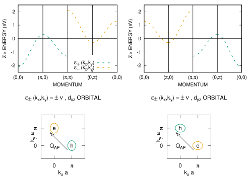
Figure 5: Renormalized electron bands and Fermi surfaces at half filling after the Lifshitz transition from Fig. 1. The staggered band shift is $\nu=1.7$ eV. The orbital character is only approximate, although it becomes exact as the area of the Fermi surface pockets vanishes as $U(\pi)$ diverges.

IV.2 Weak Electron Doping

We will now obtain solutions to the Eliashberg equations (LABEL:E_eqs) at small deviations in the electron density from half filling. In the normal state, $\Delta_{1}=0=\Delta_{2}$, the corresponding equations for the wavefunction renormalizations and for the band shifts read

$$\quad\qquad Z_{n}-1= {3\over 2}\int{d^{2}k^{\prime}\over{(2\pi)^{2}}}U^{2}(\pi){s_{1}^{2}\over{\chi_{\perp}}}{\sin^{2}[\delta({\bm{k}})+\delta({\bm{k}}^{\prime})]\over{Z_{\bar{n}}\,\omega_{b}({\bm{q}})}}\cdot$$

$$\cdot{1\over{[\omega_{b}({\bm{q}})+|\varepsilon_{+}({\bm{k}}^{\prime})-\nu_{\bar{n}}|/Z_{\bar{n}}]^{2}}},$$ (50a)

$$\nu_{n}-({\rm sgn}\,n)\mu_{0}= {3\over 2}\int{d^{2}k^{\prime}\over{(2\pi)^{2}}}U^{2}(\pi){s_{1}^{2}\over{\chi_{\perp}}}{\sin^{2}[\delta({\bm{k}})+\delta({\bm{k}}^{\prime})]\over{Z_{\bar{n}}\,\omega_{b}({\bm{q}})}}\cdot$$

$$\cdot{{\rm sgn}[\nu_{\bar{n}}-\varepsilon_{+}({\bm{k}}^{\prime})]\over{\omega_{b}({\bm{q}})+|\varepsilon_{+}({\bm{k}}^{\prime})-\nu_{\bar{n}}|/Z_{\bar{n}}}}.$$ (50b)

Above, $\nu_{1}=-\mu_{1}$ and $\nu_{2}=+\mu_{2}$ are the staggered band shifts. Also, the identity

$$\sin[\delta({\bm{k}})+\delta({\bm{k}}^{\prime})]=\sin[\delta({\bar{\bm{k}}})+\delta({\bar{\bm{k}}}^{\prime})]$$ (51)

has been applied above in the case $n=1$ for the anti-bonding ($-$) band. (See Appendix B.) Assume, in particular, that the chemical potential is positive, but small: $\mu_{0}\rightarrow 0+$. Assume, next, a linear response $\delta Z_{1}$ and $\delta Z_{2}$ with respect to the wavefunction renormalization at half filling, $Z_{1}=Z$ and $Z_{2}=Z$, along with a linear response $\delta\nu_{1}$ and $\delta\nu_{2}$ with respect to the staggered band shifts at half filling, $\nu_{1}=\nu$ and $\nu_{2}=\nu$. Taking a variation of (50) yields one linear equation per band, $n=1,2$. Adding and subtracting these yields the following linear relations in terms of even and odd variations with respect to half filling:

$$Z\,\delta Z(+) =A\,\delta Z(+)-B\,\delta\nu(+),$$

$$\quad\qquad 0 =A\,\delta Z(-)-B\,\delta\nu(-),$$ (52)

where $\delta Z(\pm)={1\over 2}(\delta Z_{2}\pm\delta Z_{1})$ and $\delta\nu(\pm)={1\over 2}(\delta\nu_{2}\pm\delta\nu_{1})$ . Here, we have constants

$$A = {3\over 2}\int{d^{2}k^{\prime}\over{(2\pi)^{2}}}U^{2}(\pi){s_{1}^{2}\over{\chi_{\perp}}}{\sin^{2}[\delta({\bm{k}})+\delta({\bm{k}}^{\prime})]\over{\omega_{b}({\bm{q}})}}{1\over{Z}}{|\varepsilon_{+}({\bm{k}}^{\prime})-\nu|/Z\over{[\omega_{b}({\bm{q}})+|\varepsilon_{+}({{\bm{k}}^{\prime}})-\nu|/Z]^{3}}},$$

$$B = {3\over 2}\int{d^{2}k^{\prime}\over{(2\pi)^{2}}}U^{2}(\pi){s_{1}^{2}\over{\chi_{\perp}}}{\sin^{2}[\delta({\bm{k}})+\delta({\bm{k}}^{\prime})]\over{\omega_{b}({\bm{q}})}}{1\over{Z}}{{\rm sgn}[\nu-\varepsilon_{+}({\bm{k}}^{\prime})]\over{[\omega_{b}({\bm{q}})+|\varepsilon_{+}({\bm{k}}^{\prime})-\nu|/Z]^{3}}}.$$

Likewise, taking a variation of (50) yields a second linear equation per band, $n=1,2$. Adding and subtracting these as well yields two more linear relations in terms of even and odd variations with respect to half filling:

$$\ \ \qquad\nu\,\delta Z(+)+Z\,\delta\nu(+) =(E-C)\delta\nu(+)+D\,\delta Z(+),$$

$$Z\mu_{0}+\nu\,\delta Z(-)-Z\delta\nu(-) =(E-C)\delta\nu(-)+D\,\delta Z(-).$$ (54)

Here, we have constants

$$C = {3\over 2}\int{d^{2}k^{\prime}\over{(2\pi)^{2}}}U^{2}(\pi){s_{1}^{2}\over{\chi_{\perp}}}{\sin^{2}[\delta({\bm{k}})+\delta({\bm{k}}^{\prime})]\over{\omega_{b}({\bm{q}})}}{1\over{Z}}{1\over{[\omega_{b}({\bm{q}})+|\varepsilon_{+}({\bm{k}}^{\prime})-\nu|/Z]^{2}}},$$

$$D = {3\over 2}\int{d^{2}k^{\prime}\over{(2\pi)^{2}}}U^{2}(\pi){s_{1}^{2}\over{\chi_{\perp}}}{\sin^{2}[\delta({\bm{k}})+\delta({\bm{k}}^{\prime})]\over{\omega_{b}({\bm{q}})}}{1\over{Z}}{{\rm sgn}[\nu-\varepsilon_{+}({\bm{k}}^{\prime})]|\varepsilon_{+}({\bm{k}}^{\prime})-\nu|/Z\over{[\omega_{b}({\bm{q}})+|\varepsilon_{+}({\bm{k}}^{\prime})-\nu|/Z]^{2}}},$$

and

$$E={3\over 2}\int{d^{2}k^{\prime}\over{(2\pi)^{2}}}U^{2}(\pi){s_{1}^{2}\over{\chi_{\perp}}}{\sin^{2}[\delta({\bm{k}})+\delta({\bm{k}}^{\prime})]\over{\omega_{b}({\bm{q}})}}{2\,\delta[\nu-\varepsilon_{+}({\bm{k}}^{\prime})]\over{\omega_{b}({\bm{q}})+|\varepsilon_{+}({\bm{k}}^{\prime})-\nu|/Z}}.$$ (56)

Collecting terms in (52) and in (54), we get

$$\delta Z(+)=-{B\over{F}}\,\delta\nu(+)\quad{\rm and}\quad\delta Z(+)=-{2Z-E\over{G}}\,\delta\nu(+)$$ (57)

in the even channel, and we get

$$\delta Z(-)={B\over{A}}\,\delta\nu(-)\quad{\rm and}\quad Z\mu_{0}=E\,\delta\nu(-)-G\,\delta Z(-)$$ (58)

in the odd channel, where $F=Z-A$ and $G=\nu-D$. These constants are then

$$F = {3\over 2}\int{d^{2}k^{\prime}\over{(2\pi)^{2}}}U^{2}(\pi){s_{1}^{2}\over{\chi_{\perp}}}{\sin^{2}[\delta({\bm{k}})+\delta({\bm{k}}^{\prime})]\over{Z}}{1\over{[\omega_{b}({\bm{q}})+|\varepsilon_{+}({\bm{k}}^{\prime})-\nu|/Z]^{3}}},$$ (59)

$$G = {3\over 2}\int{d^{2}k^{\prime}\over{(2\pi)^{2}}}U^{2}(\pi){s_{1}^{2}\over{\chi_{\perp}}}{\sin^{2}[\delta({\bm{k}})+\delta({\bm{k}}^{\prime})]\over{Z}}{{\rm sgn}[\nu-\varepsilon_{+}({\bm{k}}^{\prime})]\over{[\omega_{b}({\bm{q}})+|\varepsilon_{+}({\bm{k}}^{\prime})-\nu|/Z]^{2}}}.$$ (60)

In deriving expression (59), the first Eliashberg equation (50) at half filling $Z-1=C$ has been approximated by $Z=C$. This is exact at criticality, $\Delta_{b}\rightarrow 0$. And in deriving expression (60), the second Eliashberg equation (50) for $\nu$ at half filling has been applied.

We shall now evaluate the constants above that determine the linear response of the Eliashberg equations in the normal state driven by weak electron doping with respect to half filling: (50) and (50), as $\mu_{0}\rightarrow 0+$. Criticality is again assumed at half filling: $\Delta_{b}\rightarrow 0$. Let us begin by evaluating the constant $G$ (60). First, average it over the Fermi surface: $G\rightarrow[D_{+}(\nu)]^{-1}(2\pi)^{-2}\int_{\rm BZ}d^{2}k\,G\,\delta[\varepsilon_{+}({\bm{k}})-\nu]$. Second, replace the integrals over momentum with the product of $\Omega$ and the spectral density (LABEL:U2F) at half filling: $U^{2}F_{0}(\Omega)=\epsilon_{\rm E}/\sqrt{\Omega^{2}-\Delta_{b}^{2}}$ for $\Omega>\Delta_{b}$, and $U^{2}F_{0}(\Omega)=0$ otherwise. This yields

$$G=\int_{\Delta_{b}}^{\omega_{\rm uv}}d\Omega{\epsilon_{\rm E}\over{\sqrt{\Omega^{2}-\Delta_{b}^{2}}}}\,\Omega\int_{-W_{\rm bottom}}^{+W_{\rm top}}d\varepsilon^{\prime}Z^{-1}{{\rm sgn}(\nu-\varepsilon^{\prime})\over{[\Omega+|\varepsilon^{\prime}-\nu|/Z]^{2}}}.$$ (61)

Third, perform the first integral over the energy band $\varepsilon_{+}({\bm{k}})$ in the limit of strong on-site repulsion, $U(\pi)\rightarrow\infty$, in which case $\nu$ approaches the top of the band, $W_{\rm top}$. It is equal to $\Omega^{-1}-(W/Z+\Omega)^{-1}$. Fourth, make the change of variable $\Omega=\Delta_{b}\cosh(x)$ and take the limit $\Delta_{b}\rightarrow 0$. This yields $G=\epsilon_{\rm E}\,y\,I(y)$, where $I(y)$ is the definite integral (44a), with $y=W/\varepsilon_{\rm E}$. A closed-form expression for $I(y)$ is obtained in Appendix C.

response/variation	$\delta Z$	$\delta\nu$
$\delta Z$	$A={\varepsilon_{\rm E}\over{\Delta_{b}}}-F$ with $F={1\over 2}{\epsilon_{\rm E}\over{\Delta_{b}}}[{\pi\over 2}-I(y)-yI^{\prime}(y)]$	$B={1\over 2}{\epsilon_{\rm E}\over{\Delta_{b}^{2}}}[I^{\prime}(y)-I^{\prime}(0)]$
$\delta\nu$	$D=\nu-G$ with $G=\epsilon_{\rm E}yI(y)$	$E=\pi{\epsilon_{\rm E}\over{\Delta_{b}}}$

Table 5: Coefficients of the linear response to weak electron doping of the Eliashberg equations (50) and (50), at criticality $\Delta_{b}\rightarrow 0$: Eqs. (52) and (54). A closed form expression for the definite integral $I(y)$ is given in Appendix C, where $y=W/\varepsilon_{\rm E}$.

The remaining constants can be evaluated in a similar way. In particular, applying the same set of steps above to the expression for the constant $F$ (59) yields the definite integral

$$F={1\over 2}{\epsilon_{\rm E}\over{\Delta_{b}}}\int_{0}^{\infty}dx{1\over{\cosh x}}\Biggl{[}1-{1\over{(1+y\,{\rm sech}\,x)^{2}}}\Biggr{]}$$ (62)

at criticality, $\Delta_{b}\rightarrow 0$, where $y=W/\varepsilon_{\rm E}$. It is shown in Appendix C that (62) reduces to the closed-form expression $F={1\over 2}(\epsilon_{\rm E}/\Delta_{b})[{\pi\over 2}-I(y)-y\,I^{\prime}(y)]$, where $I^{\prime}(y)$ denotes the derivative of $I(y)$. Likewise, performing the same set of steps on the expression for the constant $B$ (IV.2) yields the definite integral

$$B={1\over 2}{\epsilon_{\rm E}\over{\Delta_{b}^{2}}}\int_{0}^{\infty}dx\Biggl{[}{1\over{(\cosh x)^{2}}}-{1\over{(y+\cosh x)^{2}}}\Biggr{]}$$ (63)

at criticality. Comparison with the definite integral (44a) therefore yields the expression $B={1\over 2}(\epsilon_{\rm E}/\Delta_{b}^{2})[I^{\prime}(y)-I^{\prime}(0)]$. And recall that a closed-form expression for the constant $A$ is obtained from that for $F$ above through the identity $A=Z-F$. Last, performing the same set of steps on the expression for the constant $E$ (56) yields the definite integral

$$E=2{\epsilon_{\rm E}\over{\Delta_{b}}}\int_{0}^{\infty}dx{1\over{\cosh x}}=\pi{\epsilon_{\rm E}\over{\Delta_{b}}}$$ (64)

at criticality. This completes the evaluation of the constants that determine the linear response of the renormalized electronic structure shown in Fig. 5 to weak electron doping at criticality, $\Delta_{b}\rightarrow 0$.

$W/W_{\rm top}$	$\varepsilon_{\rm E}/W$	$\epsilon_{\rm E}/W$	$\chi_{\rm E}$	$X_{\rm E}W$
$1.0$	$0.343$	$0.366$	$2.045$	$8.671$
$1.1$	$0.298$	$0.303$	$2.120$	$9.673$
$1.2$	$0.261$	$0.255$	$2.200$	$10.780$
$1.3$	$0.231$	$0.218$	$2.284$	$12.001$
$1.4$	$0.206$	$0.189$	$2.373$	$13.344$
$1.5$	$0.185$	$0.165$	$2.467$	$14.821$

Table 6: Numerical solutions of Eliashberg equations at half filling, at criticality, in the limit $U(\pi)\rightarrow\infty$: Eq. (45). Also listed are the susceptibilities about half filling: $\delta\mu_{1}=\chi_{\rm E}\,\mu_{0}=\delta\mu_{2}$ and $\delta Z_{2}/Z=X_{\rm E}\mu_{0}=-\delta Z_{1}/Z$. Note that $W/W_{\rm top}=1+(t_{1}^{\parallel}/t_{1}^{\perp})$.

In conclusion, at weak electron doping, the normal-state Eliashberg equations (50) and (50) yield independent linear-response equations in the even and in the odd channels, (57) and (58). The coefficients of the linear response are summarized by Table 5. In the even channel, we thereby get $\delta Z(+)=0$ and $\delta\nu(+)=0$ if $BG\neq(2Z-E)F$. Notice that $B$, $G$ and $F$ are positive, while $2Z-E=(2\varepsilon_{\rm E}-\pi\epsilon_{\rm E})/\Delta_{b}$ is negative by Table 6. The former inequality is therefore valid, and we get $\delta Z_{1}=-\delta Z_{2}$ and $\delta\mu_{1}=\delta\mu_{2}$. And in the odd channel, (58) yields

$$\delta Z(-)=\chi_{\rm E}{B\over A}\mu_{0}\quad{\rm and}\quad\delta\nu(-)=\chi_{\rm E}\,\mu_{0},$$ (65)

with susceptibility $\chi_{\rm E}=Z/(E-{BG\over{A}})$. The latter can be calculated from the previous closed-form expressions for the constants $A$ thru $G$ that are listed in Table 5, and the results are listed in Table 6. Importantly, $\chi_{\rm E}$ is positive at $W/W_{\rm top}$ between $1.0$ and $1.5$, which corresponds to at most weak eccentricity in the electron/hole Fermi surface pockets at the corner of the two-iron Brillouin zone. Recall that $\delta\nu(-)={1\over 2}(\delta\mu_{1}+\delta\mu_{2})$ is the average chemical-potential shift, which is equal to $\delta\mu_{1}=\delta\mu_{2}$. The latter and (65) therefore imply a rigid shift of the renormalized electronic structure at half filling by a chemical-potential shift proportional to the electron doping. Figure 6 is such a rigid shift of Fig. 5. Also recall that $\delta Z(-)={1\over 2}(\delta Z_{2}-\delta Z_{1})$, which is equal to $\delta Z_{2}=-\delta Z_{1}$. Upon electron doping, the latter and (65) imply, on the other hand, that the wavefunction renormalization increases with respect to $Z=\varepsilon_{\rm E}/\Delta_{b}$ on the hole Fermi surface pockets ($n=2$), while that it decreases with respect to $Z$ on the electron Fermi surface pockets ($n=1$). The magnitude of the equal and opposite variation in the wavefunction renormalization is best stated as $\delta Z(-)/Z=X_{\rm E}\mu_{0}$, where $X_{\rm E}={B\over A}/(E-{BG\over A})$. The values of $X_{\rm E}W$ listed in Table 6 suggest that $Z_{1}\mathrel{\scriptstyle{\buildrel>\over{\sim}}}1$ and that $Z_{2}\sim 2Z$ at electron doping greater than $x_{0}$. This will be discussed at length below and in the next section.

Yet what is the superconducting gap at weak electron doping with respect to half filling? Inspection of the gap equations in the Eliashberg equations (LABEL:E_eqs) yields that they are equivalent to the ones at half filling to linear order in the variations $\delta Z_{1}$, $\delta Z_{2}$, $\delta\mu_{1}$ and $\delta\mu_{2}$, and in the gaps $\Delta_{1}$ and $\Delta_{2}$. Because $\Delta_{1}$ and $\Delta_{2}$ are null at half filling, the linear susceptibility of these quantities with electron doping $\mu_{0}>0$ is also null. Any superconducting gap that opens at weak electron doping must therefore depend non-linearly on the doping concentration. (See Fig. 7.)

IV.3 Moderate Electron Doping

Let us next seek solutions to the Eliashberg equations, (36-36), at moderate electron doping $x\sim x_{0}$. The previous linear response due to weak electron doping predicts a rigid shift in energy of the renormalized electronic structure at half filling displayed by Fig. 5. It is depicted by Fig. 6, where the top of the bonding ($+$) band lies just above the Fermi level. The previous linear response about half filling also predicts wavefunction renormalizations $Z_{2}$ and $Z_{1}$ for the bonding band ($n=2$) and for the anti-bonding band ($n=1$), respectively, above and below the unique value at half filling. What then does the third Eliashberg equation for the superconducting gap (36) predict at moderate doping?

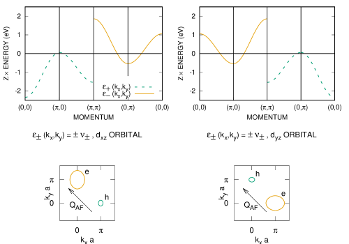
Figure 6: Renormalized electron bands and Fermi surfaces at electron doping after the Lifshitz transition. Again, the orbital character is only approximate.

We shall follow the historical approach for the solution of the Eliashberg equations in the case of the electron-phonon interactionschrieffer_64 ; scalapino_69 ; morel_anderson_62 ; mcmillan_68 ; ginzburg_kirzhnits_82 ; carbotte_90 . In particular, before confronting the gap equation, it is useful first to obtain the wavefunction renormalizations of the two bands at the Fermi level in the normal state. Neglecting frequency dependence, the first Eliashberg equation (36) then yields the following wavefunction renormalizations at the Fermi level, $\omega=0$:

$$Z_{n}-1=\int_{\Delta_{b}}^{\omega_{\rm uv}}d\Omega\,U^{2}F_{0}^{(n,{\bar{n}})}(\Omega,\mu_{n},\mu_{\bar{n}})\Biggl{(}{1\over{\Omega}}-{1\over{W/Z_{\bar{n}}+\Omega}}\Biggr{)}.$$ (66)

Again, the order of integration in (36) has been reversed. Next, assume weak to moderate wavefunction renormalization in the anti-bonding ($-$) band and strong wavefunction renormalization in the bonding ($+$) band: $\lambda_{1}$ such that $W/Z_{1}\gg\Delta_{b}$, and $\lambda_{2}\gg 1$ such that $W/Z_{2}\ll\Delta_{b}$. Here $\lambda_{n}=Z_{n}-1$. Notice that the last inequality is consistent with the previous results at weak electron doping: $\varepsilon_{\rm E}/\Delta_{b}<Z_{2}$. The above Eliashberg equations (66) then yield the results

$$\lambda_{2}\cong\int_{\Delta_{b}}^{\omega_{\rm uv}}d\Omega\,\Omega^{-1}U^{2}F_{0}^{(2,1)}(\Omega,\mu_{2},\mu_{1}),$$ (67)

and

$$\lambda_{1}\cong{W\over{Z_{2}}}\int_{\Delta_{b}}^{\omega_{\rm uv}}d\Omega\,\Omega^{-2}U^{2}F_{0}^{(1,2)}(\Omega,\mu_{1},\mu_{2}),$$ (68)

or $\lambda_{1}\cong(W/Z_{2})\lambda_{2}\,{\overline{\Omega^{-1}}}$. The distribution in the average ${\overline{\Omega^{-1}}}$ is normalized by the integral (67) because of the approximate identity $U^{2}F_{0}^{(1,2)}(\Omega,\mu_{1},\mu_{2})\cong U^{2}F_{0}^{(2,1)}(\Omega,\mu_{2},\mu_{1})$. By (LABEL:U2F), the latter is due to the approximate identity obeyed by the density of states, $D_{-}(\mu_{1})\cong D_{+}(\mu_{2})$, at $\mu_{1}$ and $\mu_{2}$ near the bottom and near the top of the respective bands $\varepsilon_{-}({\bm{k}})$ and $\varepsilon_{+}({\bm{k}})$. Here, also, we have applied the identity (51). Because $\lambda_{2}\gg 1$, we then have that $\lambda_{1}\cong W\,{\overline{\Omega^{-1}}}$. Finally, the initial assumption of moderate $\lambda_{1}$ is confirmed by noting that $W/Z_{1}\cong W/(1+W\,{\overline{\Omega^{-1}}})\cong({\overline{\Omega^{-1}}})^{-1}$, which is much greater than $\Delta_{b}$.

We shall now show that an instability to $S$-wave Cooper pairing exists that alternates in sign between the strong electron-type Fermi surface of the anti-bonding ($-$) band, $n=1$, and the weak hole-type Fermi surface of the bonding ($+$) band, $n=2$. (See Fig. 6.) In particular, assume the simple BCS form (47) for the frequency dependence of the respective gaps, $\Delta_{1}(\omega)$ and $\Delta_{2}(\omega)$, with frequency cutoffs $\omega_{c}(1)$ and $\omega_{c}(2)$. After neglecting the frequency dependence of the wavefunction renormalizations, the gap equations (36) then read

$$Z_{n}\Delta_{n}=-2\int_{|\Delta_{\bar{n}}|}^{\omega_{c}({\bar{n}})}dE^{\prime}{\Delta_{\bar{n}}\over{\sqrt{E^{\prime 2}-\Delta_{\bar{n}}^{2}}}}\int_{\Delta_{b}}^{\omega_{\rm uv}}d\Omega\,U^{2}F_{0}^{(n,{\bar{n}})}(\Omega;\mu_{n},\mu_{\bar{n}}){1\over{\Omega+E^{\prime}}}.$$

(69)

Assume, further, the BCS limit: $\omega_{c}(1),\omega_{c}(2)\rightarrow 0$. Taking the normal-state values for the wavefunction renormalizations discussed above is then valid. Also, the denominator above, $\Omega+E^{\prime}$, can then be replaced by $\Omega$. After comparison with (67), we thereby arrive at the gap equations

$$Z_{n}\Delta_{n}=-2\int_{|\Delta_{\bar{n}}|}^{\omega_{c}({\bar{n}})}dE^{\prime}{\lambda_{2}\over{\sqrt{E^{\prime 2}-\Delta_{\bar{n}}^{2}}}}\Delta_{\bar{n}},$$ (70)

or $\Delta_{1}=-K_{1,2}\Delta_{2}$ and $\Delta_{2}=-K_{2,1}\Delta_{1}$, with kernels

$$K_{1,2} = 2{\lambda_{2}\over{Z_{1}}}\sinh^{-1}\Biggl{[}{\sqrt{\omega_{c}^{2}(2)-\Delta_{2}^{2}}\over{|\Delta_{2}|}}\Biggr{]}\quad{\rm and}\quad$$

$$K_{2,1} = 2{\lambda_{2}\over{Z_{2}}}\sinh^{-1}\Biggl{[}{\sqrt{\omega_{c}^{2}(1)-\Delta_{1}^{2}}\over{|\Delta_{1}|}}\Biggr{]}.$$

Importantly, these equations imply that $\Delta_{1}$ and $\Delta_{2}$ are of opposite sign! An $S^{+-}$ pairing instability therefore exists between the strong and the weak Fermi surfaces shown in Fig. 6.

To obtain explicit solutions of the gap equations, it is useful to multiply and divide these, which yields

$$1=K_{1,2}K_{2,1}\quad{\rm and}\quad\Bigl{(}{\Delta_{2}\over{\Delta_{1}}}\Bigr{)}^{2}={K_{2,1}\over{K_{1,2}}}.$$ (72)

Taking the product of the above then gives $|\Delta_{2}/\Delta_{1}|=K_{2,1}\cong 2\sinh^{-1}[\sqrt{\omega_{c}^{2}(1)-\Delta_{1}^{2}}/|\Delta_{1}|]$. Assuming $|\Delta_{1}|$ near $\omega_{c}(1)$ in turn yields $|\Delta_{2}|\cong 2\sqrt{2\omega_{c}(1)}\sqrt{\omega_{c}(1)-|\Delta_{1}|}$. Substituting the previous into the first gap equation displayed by (72) then yields

$$1\cong 2{\lambda_{2}\over{Z_{1}}}{|\Delta_{2}|\over{\omega_{c}(1)}}\sinh^{-1}\biggl{[}{\omega_{c}(2)\over{|\Delta_{2}|}}\biggl{]},$$ (73)

or $|\Delta_{2}|\sim(Z_{1}/Z_{2})|\Delta_{1}|$, with $|\Delta_{1}|\cong\omega_{c}(1)$. This solution thereby confirms the instability of the Fermi surfaces to $S^{+-}$ pairing, where the wavefunction renormalization $Z_{1}$ on the larger electron-type Fermi surface is of moderate size compared to unity, while the wavefunction renormalization $Z_{2}$ on the smaller hole-type Fermi surface is large compared to unity. (See Fig. 6.)

V Discussion

The previous results of electron Fermi surface pockets and faint hole Fermi surface pockets at the corner of the folded (two-iron) Brillouin zone, with $S^{+-}$ Cooper pairing that alternates in sign between them, is compared below to a local-moment model for electron-doped iron selenide and to high-temperature iron-selenide superconductors themselves.

V.1 Comparison with Local-Moment Model

A local-moment model of the electronic physics in electron-doped iron selenide exists that captures many of the principal features of the above Eliashberg theoryjpr_17 . It emerges near half filling in the strong correlation limit, $U_{0}\rightarrow\infty$. By (13), isospin symmetry is broken strongly along the $I^{(3)}$ axis in such a case. In particular, doubly occupied orbital states listed in Table 1 are projected out. The following Hund-Heisenberg model in terms of the spin operators ${\bm{S}}_{i,d+}$ and ${\bm{S}}_{i,d-}$ then accurately describes the spin dynamicsjpr_10 :

$$H_{\rm HH}= \sum_{i}J_{0}{\bm{S}}_{i,d-}\cdot{\bm{S}}_{i,d+}+\sum_{\langle i,j\rangle}(J_{1}^{\parallel}{\bm{S}}_{i,\alpha}\cdot{\bm{S}}_{j,\alpha}+J_{1}^{\perp}{\bm{S}}_{i,\alpha}\cdot{\bm{S}}_{j,{\bar{\alpha}}})$$ (74)

$$+\sum_{\langle\langle i,j\rangle\rangle}(J_{2}^{\parallel}{\bm{S}}_{i,\alpha}\cdot{\bm{S}}_{j,\alpha}+J_{2}^{\perp}{\bm{S}}_{i,\alpha}\cdot{\bm{S}}_{j,\bar{\alpha}}).$$

Here the index $\alpha$ is implicitly summed over the iron ${d+}$ and ${d-}$ orbitals. The intra-orbital ($\parallel$) and inter-orbital ($\perp$) Heisenberg exchange coupling constants are positive, and they satisfy $J_{1}^{\parallel}>J_{1}^{\perp}$ and $J_{2}^{\parallel}=J_{2}^{\perp}$. The above spin Hamiltonian also contains Hund’s Rule exchange coupling between the orbitals, with a ferromagnetic coupling constant, $J_{0}<0$. Again, the infinite-$U_{0}$ limit is taken, which means that the formation of spin singlets per site, per $d+$ or $d-$ orbital, is suppressed. Electron hopping via the Hamiltonian $H_{\rm hop}$ (1) is also added at electron doping, but in the infinite-$U_{0}$ limit. Last, notice that orbital swap, $d-\leftrightarrow d+$, is a global symmetry of the Hund-Heisenberg Hamiltonian (74). It is therefore most natural to consider the case where orbital swap $P_{d,{\bar{d}}}$ is a global symmetry of the hopping Hamiltonian $H_{\rm hop}$ (1) as well. This requires the absence of mixing between the $3d_{xz}$ and $3d_{yz}$ orbitals: $t_{2}^{\perp}=0$. The latter restriction for the validity of the two-orbital $t$-$J$ model emerges from the underlying extended Hubbard model in the large-$U_{0}$ limit at half fillingjpr_rm_18 . In such case, for example, the transverse spin susceptibilities of both models, $\chi_{\perp}$, coincide only in the limit $t_{2}^{\perp}/i\rightarrow 0$.

The author exploited the Schwinger-boson-slave-fermion representation of the correlated electron to study the above local-moment modeljpr_17 . Here, the correlated electron fractionalizes into a Schwinger boson that carries spin and a slave fermion that carries charge. At half filling, an hSDW of the type depicted by Fig. 3b is predicted at $J_{1}^{\parallel}>J_{1}^{\perp}$ and at Hund’s Rule exchange couplingjpr_17 ; jpr_10 , $-J_{0}$, below a critical one. In particular, a quantum-critical point exists at moderate Hund’s Rule coupling $-J_{0c}$, where the spin-excitation spectrum collapses to zero energy at stripe SDW wave numbers $(\pi/a,0)$ and $(0,\pi/a)$. Specifically, the QCP occurs atjpr_17 ; jpr_10

$$-J_{0c}=2(J_{1}^{\parallel}-J_{1}^{\perp})+2t_{1}^{\perp}x/(1-x)^{2}s_{0}-4J_{2}^{\parallel}$$ (75)

in the minimal case where only the $t_{1}^{\perp}({\hat{\bm{x}}})=-t_{1}^{\perp}({\hat{\bm{y}}})$ hopping matrix elements are non-zero. Here, $x$ denotes the concentration of electron doping from half filling, while $s_{0}$ denotes the spin of the electron. The quantum-critical line (75) is depicted by the dashed line in Fig. 7. It is possible to identify the critical normal state of the previous Eliashberg theory at half filling ($\Delta_{b}$, $\Delta_{1}$, and $\Delta_{2}\rightarrow 0$) with this QCP.

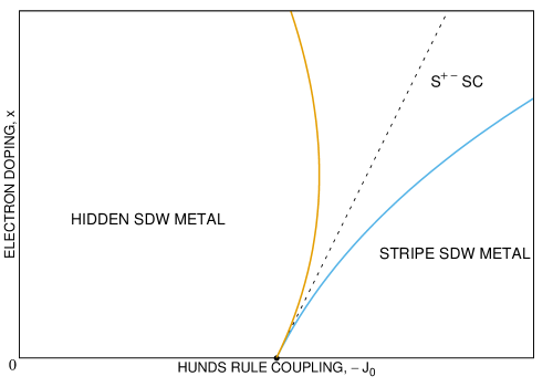
Figure 7: Proposed phase diagram for local-moment model of electron-doped iron selenide (ref. jpr_17 ). The latter predicts the phase boundary approaching half filling (dashed line), which separates the hSDW state from the stripe SDW state. The intervening $S^{+-}$ superconducting phase is predicted by the Eliashberg Theory introduced in the main text.

Both Schwinger-boson-slave-fermion mean field theory about the hidden Néel state and exact calculations on finite clusters for the above local-moment model find evidence for a $d_{xz}$ and a $d_{yz}$ Fermi-surface pocket at the corner of the two-iron Brillouin zone, at electron dopingjpr_17 . This result agrees with the previous results based on Eliashberg Theory, which are summarized by Fig. 6. Yet how does the area of the slave-fermion Fermi-surface pockets compare with that predicted by the previous Eliashberg theory, Fig. 6 ? Because the slave fermions do not carry spin, we have by charge conservation that

$$[D_{+}({\rm top})+D_{-}({\rm bottom})]\delta\mu=2[D_{+}(0)+D_{-}(0)]\mu_{0}.$$ (76)

The left-hand and the right-hand sides above correspond, respectively, to the cases where interactions are turned on (Fig. 5) and turned off (Fig. 1). In the above Eliashberg theory, (36)-(36) and (LABEL:U2F), it has been assumed throughout that $D_{+}(\varepsilon)\cong D_{+}({\rm top})$ and that $D_{-}(\varepsilon)\cong D_{-}({\rm bottom})$, however. Within that approximation, (76) thereby yields the susceptibility

$$\chi_{\rm E}={\delta\mu\over{\mu_{0}}}\cong 2$$

from the Schwinger-boson-slave-fermion mean field theory. It agrees with the corresponding result from Eliashberg theory listed in Table 6, at hopping matrix element $t_{1}^{\parallel}\rightarrow 0$, in which case the renormalized Fermi-surface pockets become perfectly circular as $U_{0}$ grows large ($x_{0}\rightarrow 0$). This coincides with the hopping parameters studied in the local-moment model within the mean-field approximationjpr_17 , in which case only $t_{1}^{\perp}$ is non-zero.

And how do the predictions for wavefunction renormalization by the previous Eliashberg theory compare with the local-moment modeljpr_17 ? A faint hole band with quasi-particle weight $1/Z_{2}$ that vanishes at criticality, $\Delta_{b}\rightarrow 0$, is predicted by Eliashberg theory. (See Fig. 6.) It crosses the Fermi level near the corner of the folded (two-iron) Brillouin zone. At electron doping, both mean field theory and exact calculations on finite clusters find no evidence for low-energy hole excitations in the two-orbital $t$-$J$ model at momenta $(\pi/a,0)$ and $(0,\pi/a)$. This is consistent with the previous. Also, in the limit of large electron spin $s_{0}$, Schwinger-boson-slave-fermion mean field theory yields a coherent contribution to the one-particle Greens function equal to $G_{\rm coh}({\bm{k}},\omega)=s_{0}/[\omega+\mu_{1}-\varepsilon_{-}({\bm{k}})].$ This is also consistent with the appreciable quasi-particle weight $1/Z_{1}$ predicted by Eliashberg theory at electron doping for the electron-type Fermi surface pockets at the corner of the two-iron Brillouin zone.

Last, exact calculations of the local-moment model for electron-doped FeSe on finite clusters find evidence for an $S$-wave Cooper pair at an energy below a continuum of states near the QCPjpr_17 . This is consistent with the prediction made above by Eliashberg theory for an instability of the Fermi surface to $S^{+-}$ superconductivity. The former exact calculations also find a $D$-wave Cooper pair at an energy below the continuum of states, but lying above the $S$-wave Cooper pair. The separation in energy between the two pair states collapses to zero at the QCP.

Finally, the Schwinger-boson-slave-fermion mean field theory for the local-moment model assumes only inter-orbital nearest neighbor hopping between iron atomsjpr_17 , $t_{1}^{\perp}({\bm{\hat{x}}})=-t_{1}^{\perp}({\bm{\hat{y}}})$. Such hopping of electrons leaves the two sublattices of the hidden Néel order displayed by Fig. 3b intact. Yet intra-orbital hopping of electrons across next-nearest neighbors, $t_{2}^{\parallel}$, also leaves the sublattices for hidden Néel order intact. Switching it on then leaves the predictions for the local-moment model mentioned abovejpr_17 unchanged. Direct calculation of the Schwinger-boson-slave-fermion mean field theory confirms this claim for $|t_{1}^{\perp}|>2t_{2}^{\parallel}$. Because the results of the local-moment model coincide with those of the Eliashberg Theory for the extended Hubbard model obtained in the previous section, we believe that the latter can remain valid off perfect nesting (7), at $t_{2}^{\parallel}\neq 0$.

V.2 Comparison with Experiment

The prediction displayed by Fig. 6 of electron-type Fermi surface pockets centered at the corner of the two-iron Brillouin zone agrees with ARPES on electron-doped iron selenideqian_11 ; liu_12 ; niu_15 . Eliashberg theory also predicts the opening of an $S$-wave gap over such Fermi surface pockets, which also agrees with ARPES on these systemsxu_12 ; peng_14 ; lee_14 ; zhao_16 , as well as with STMxue_12 ; fan_15 ; yan_15 . Electron-electron interactions are expected to be moderately strong in iron selenide. This rules out conventional $S$-wave pairing over the electron Fermi surface pockets in electron-doped iron selenide. The $S^{+-}$ Cooper pairing that is predicted here between the electron Fermi surface pockets and faint hole Fermi surface pockets at the corner of the folded Brillouin zone therefore potentially resolves the puzzling observations of isotropic pair gaps in electron-doped iron selenide. In particular, the frequency cutoff for the hidden spin fluctuations that appears in the gap equations (LABEL:K)-(73) obtained from Eliashberg Theory is approximately $\omega_{c}(1)\cong 2k_{F1}c_{b}=2(2\pi x_{1})^{1/2}c_{b}/a$ in the case of the anti-bonding band, $n=1$, where $x_{1}$ denotes the concentration of each electron pocket. The Hund-Heisenberg model (74) at half filling predicts a hidden-spin-wave velocity in the hSDW state ofjpr_10

$$c_{b}/a=2s_{1}\Bigl{[}\Bigl{(}J_{1}^{\parallel}-J_{1}^{\perp}\Bigr{)}\Bigl{(}{1\over 2}J_{0}+2J_{1}^{\parallel}+2J_{2}^{\perp}\Bigr{)}\Bigr{]}^{1/2},$$ (77)

at $J_{2}^{\parallel}=J_{2}^{\perp}$. ARPES on electron-doped iron selenide finds a gap in the range $\Delta_{1}=10$-$20$ meV at zero temperaturexu_12 ; peng_14 ; lee_14 ; zhao_16 . Let us set $J_{1}^{\perp}=0$ and assume values for the remaining Heisenberg exchange coupling constants and the Hund’s Rule exchange coupling constant of orderjpr_10 $|J_{0}|,J_{1}^{\parallel},J_{2}^{\parallel}=J_{2}^{\perp}\sim 100$ meV. At moderately small electron pockets, $2(2\pi x_{1})^{1/2}\sim 1$, this then yields a gap $\Delta_{1}\cong\omega_{c}(1)$ that is of order the gap determined by ARPES for low ordered moments, $s_{1}<1/2$.

The spectrum of hidden spin fluctuations centered at the antiferromagnetic wave number ${\bm{Q}}_{\rm AF}=(\pi/a,\pi/a)$ is what binds together electrons into $S^{+-}$ Cooper pairs in the present Eliashberg theory. Recent inelastic neutron scattering studies on intercalated iron selenidepan_17 find low-energy magnetic excitations at wave numbers around ${\bm{Q}}_{\rm AF}$, but no low-energy spin excitations at ${\bm{Q}}_{\rm AF}$. Such a ring of low-energy magnetic excitations is in fact consistent with the low-energy hidden spin fluctuations that are exploited by the present Eliashberg theory. In particular, both the two-orbital local-moment model discussed above and the underlying extended Hubbard model for electron-doped iron selenide described in subsection II.2 predict that the low-energy hidden spin fluctuations centered at ${\bm{Q}}_{\rm AF}$ are not observable in the true-spin channel of the iron atomsjpr_rm_18 ; jpr_20a . This leaves a ring of observable spin excitations around the antiferromagnetic wavevector ${\bm{Q}}_{\rm AF}$, in agreement with inelastic neutron scatteringpan_17 .

V.3 Iron $3d_{xy}$ Orbital, Buried Hole Bands, and Polarization Correction

Although the present study suggests that the iron $3d_{xz}/3d_{yz}$ orbitals are the principal ones in electron-doped iron selenide, ARPES and density-functional theory indicate that the iron $3d_{xy}$ orbital also plays an important roleyi_15 . Indeed, it is quite possible that the two $3d_{xz}/3d_{yz}$ bands and the $3d_{xy}$ band are approximately half filled in electron-doped iron selenideLee_Wen_08 ; Yu_Si_13 . Doubly occupied $3d_{x^{2}-y^{2}}$ and $3d_{x^{2}+y^{2}-2z^{2}}$ orbitals are consistent with such fillings among the iron $3d$ bands. Electron doping could achieve an atomic configuration [Ar]$3d^{7}4s^{2}$ for Fe^-, which in turn is consistent with such occupancies among the $3d$ orbitals. A relatively flat and hole-type $3d_{xy}$ band can be added to the present Eliashberg Theory for $3d_{xz}/3d_{yz}$ electrons interacting with hidden spin fluctuations (Fig. 4). (See ref. sup_mat , Fig. S1.) Because electrons in the $3d_{xy}$ band do not interact with hidden spin fluctuations, they may be considered to be spectators. Weak mixing of the two $3d_{xz}/3d_{yz}$ bands with the $3d_{xy}$ band results in the expected level repulsion of the renormalized electron/hole Fermi surface pockets shown in Fig. 5. (See ref. sup_mat , Fig. S3.) This implies that the Lifshitz transition to such a renormalized band structure at half filling is robust in the presence of weak mixing with the $3d_{xy}$ band. Also, within the present Eliashberg Theory, a direct calculation of the propagator for such $3d_{xy}$ spectator electrons finds that they inherit divergent wavefunction renormalization at the Fermi level from the $3d_{xz}/3d_{yz}$ electrons at half filling. (See ref. sup_mat , Eq. (S20).) In particular, the vanishing quasi-particle weight of the $3d_{xz}/3d_{yz}$ electrons at the Fermi level, $Z^{-1}\rightarrow 0$, implies the vanishing quasi-particle weight of the $3d_{xy}$ electrons at the Fermi level. (Cf. ref. Yu_Si_13 .) Similar results are obtained when the spin-orbit interaction is included on iron atoms that are strictly equivalent over the square latticesup_mat . Last, the tips of the electron Fermi surface pockets ($n=1$) shown in Fig. 5 can acquire $3d_{xy}$ orbital character if the electron/hole Fermi surface pockets are large enough. This coincides with predictions made by band-structure calculations on alkali-atom intercalated iron selenidesmaier_11 ; mazin_11 .

ARPES on electron-doped iron selenide finds hole-type bands at the center of the unfolded Brillouin zone that lie below the bottom of the electron-type bands at the corner of the folded Brillouin zoneqian_11 ; liu_12 ; lee_14 ; zhao_16 ; niu_15 . Schwinger-boson-slave-fermion mean field theory of the local-moment model mentioned previously finds evidence for incoherent hole bands buried below the Fermi level at the $\Gamma$-point as welljpr_17 . The present calculations based on Eliashberg theory do not predict such hole-type bands, however. Figure 1 shows bare bonding and anti-bonding bands near the Fermi level that become degenerate at momenta ${\bm{k}}=(0,0)$ and $(\pi/a,\pi/a)$ in the unfolded Brillouin zone. The two bands show opposite curvatures at these points when the hybridization between the $3d_{xz}$ and $3d_{yz}$ orbitals lies inside the window $t_{1}^{\parallel}<2|t_{2}^{\perp}|<|t_{1}^{\perp}|$. It is possible that including momentum and/or frequency dependence in the present Eliashberg Theory opens a gap at the Fermi level at these $\Gamma$-points in momentum space. Such a calculation lies outside the scope of the present one, however.

Absent from the previous calculations of the electron self-energy corrections within Eliashberg Theory, Fig. 4, is the polarization correctionschrieffer_64 ; scalapino_69 to the propagator (15) for hidden spinwaves. Recall the wavefunction renormalization for electrons near the Fermi surface at half filling: $Z=\varepsilon_{\rm E}/\Delta_{b}$. The former polarization correction therefore vanishes at the QCP, where $\Delta_{b}\rightarrow 0$. Proximity to the QCP is assumed throughout, which justifies the neglect of the polarization correction to the propagation of hidden spinwaves.

VI Conclusions

We have shown above how low-energy hidden spin fluctuations near the wavevector for the checkerboard on the square lattice of iron atoms in electron-doped iron selenide lead to superconductivity, with isotropic Cooper pairs that alternate in sign between strong electron Fermi surface pockets and faint hole Fermi surface pockets. (See Fig. 6.) By contrast with the incipient-band mechanism for $S^{+-}$ superconductivitylinscheid_16 , the latter do not coincide with the hole bands buried below the Fermi level at the center of the Brillouin zone. Both electron and hole Fermi surface pockets lie at the corner of the folded (two-iron) Brillouin zone. A comparison of the gap that is predicted to open over the electron Fermi surface pockets with that observed by ARPESxu_12 ; peng_14 ; lee_14 ; zhao_16 is consistent with short-range hidden magnetic order, with a moderate to weak ordered moment.

Like true spin fluctuations in the case of iron-pnictide materialsmazin_08 ; kuroki_08 ; graser_09 , the hidden spin fluctuations studied here are due to nested Fermi surfaces. In the present case, however, the exchange of hidden spin fluctuations give rise to significant band shifts. In particular, Eliashberg theory reveals that they incite a Lifshitz transition from nested Fermi surfaces at the center and at the corner of the unfolded (one-iron) Brillouin zone to nested Fermi surfaces at the corner of the folded Brillouin zonejpr_rm_18 . Also, like true spin fluctuations in the case of iron-pnictide materialsmazin_08 ; kuroki_08 ; graser_09 ; dolgov_09 ; benfatto_09 ; ummarino_09 , hidden spin fluctuations give rise to repulsive inter-band interactions between electrons that favor $S^{+-}$ Cooper pairing between the renormalized Fermi surface pockets. In the present case, however, orbital matrix elements result in weak effective inter-band interactions. This justifies the neglect of vertex corrections in Eliashberg theoryschrieffer_64 ; scalapino_69 .

It has also been recently argued by the author that hidden spin fluctuations account for the ring of low-energy spin excitations at the checkerboard wavevector observed by inelastic neutron scattering in electron-doped iron selenidejpr_20a ; pan_17 . This, coupled with the prediction of $S^{+-}$ superconductivity described above, suggests that hidden spin fluctuations play an important role in high-temperature iron-selenide superconductors.

Appendix A Spin and Isospin Operators

The spin operator at iron site $i$ and orbital $\alpha$ is the usual contraction of Pauli matrices ${\bm{\sigma}}$ over spin quantum numbers:

$${\bm{S}}_{i,\alpha}={\hbar\over 2}\sum_{s=\uparrow,\downarrow}\sum_{s^{\prime}=\uparrow,\downarrow}c_{i,\alpha,s}^{\dagger}{\bm{\sigma}}_{s,s^{\prime}}c_{i,\alpha,s^{\prime}}.$$ (78)

The spin operator at iron site $i$ is then

$${\bm{S}}_{i}={\bm{S}}_{i,d+}+{\bm{S}}_{i,d-}.$$ (79)

The isospin operator at iron site $i$ and for spin $s$, on the other hand, is the contraction of Pauli matrices ${\bm{\tau}}$ over the two orbital quantum numbers:

$${\bm{I}}_{i,s}={1\over 2}\sum_{\alpha={d+},{d-}}\sum_{\alpha^{\prime}={d+},{d-}}c_{i,\alpha,s}^{\dagger}{\bm{\tau}}_{\alpha,\alpha^{\prime}}c_{i,\alpha^{\prime},s}.$$ (80)

The isospin operator at iron site $i$ is then

$${\bm{I}}_{i}={\bm{I}}_{i,\uparrow}+{\bm{I}}_{i,\downarrow}.$$ (81)

Last, the operator for the tensor product of the spin with isospin is the contraction of ${\bm{\sigma}}{\bm{\tau}}$ over both the spin and isospin quantum numbers:

$$({\bm{S}}\otimes{\bm{I}})_{i}={\hbar\over 4}\sum_{s=\uparrow,\downarrow}\sum_{\alpha={d+},{d-}}\sum_{\alpha^{\prime}={d+},{d-}}\sum_{s^{\prime}=\uparrow,\downarrow}c_{i,\alpha,s}^{\dagger}{\bm{\sigma}}_{s,s^{\prime}}{\bm{\tau}}_{\alpha,\alpha^{\prime}}c_{i,\alpha^{\prime},s^{\prime}}.$$ (82)

Appendix B Orbital Matrix Element

The operators that create the eigenstates (5) of the electron hopping Hamiltonian, $H_{\rm hop}$, are

$$c_{s}^{\dagger}(n,{\bm{k}})={\cal N}^{-1/2}\sum_{i}\sum_{\alpha=0,1}(-1)^{\alpha n}e^{i(2\alpha-1)\delta(\bm{k})}e^{i{\bm{k}}\cdot{\bm{r}}_{i}}c_{i,\alpha,s}^{\dagger},$$ (83)

where $\alpha=0$ and $1$ index the $d-$ and $d+$ orbitals, and where $n=1$ and $2$ index the anti-bonding and bonding orbitals $(-i)d_{y(\delta)z}$ and $d_{x(\delta)z}$. The inverse of the above is then

$$c_{i,\alpha,s}^{\dagger}={\cal N}^{-1/2}\sum_{\bm{k}}\sum_{n=1,2}(-1)^{\alpha n}e^{-i(2\alpha-1)\delta({\bm{k}})}e^{-i{\bm{k}}\cdot{\bm{r}}_{i}}c_{s}^{\dagger}(n,{\bm{k}}).$$ (84)

Plugging (84) and its hermitian conjugate into the expression for the hidden electron spin operator,

$${\bm{S}}(\pi,{\bm{q}})={1\over 2}\sum_{s}\sum_{s^{\prime}}\sum_{i}\sum_{\alpha}(-1)^{\alpha}e^{i{\bm{q}}\cdot{\bm{r}}_{i}}c_{i,\alpha,s}^{\dagger}{\bm{\sigma}}_{s,s^{\prime}}c_{i,\alpha,s^{\prime}},$$ (85)

yields the form

$${\bm{S}}(\pi,{\bm{q}})={1\over 2}\sum_{s}\sum_{s^{\prime}}\sum_{\bm{k}}\sum_{n,n^{\prime}}{\cal M}_{n,{\bm{k}};n^{\prime},{\bm{k}}^{\prime}}\,c_{s}^{\dagger}(n^{\prime},{\bm{k}}^{\prime}){\bm{\sigma}}_{s,s^{\prime}}c_{s^{\prime}}(n,{\bm{k}}),$$

(86)

with the matrix elementjpr_rm_18

$${\cal M}_{n,{\bm{k}};n^{\prime},{\bm{k}}^{\prime}}=\begin{cases}-i\,\sin[\delta({\bm{k}})-\delta({\bm{k}}^{\prime})]&{\rm for}\quad n^{\prime}=n,\\ \cos[\delta({\bm{k}})-\delta({\bm{k}}^{\prime})]&{\rm for}\quad n^{\prime}\neq n.\end{cases}$$ (87)

Here, ${\bm{k}}^{\prime}={\bm{k}}-{\bm{q}}$. Now replace ${\bm{k}}^{\prime}$ above with ${\bar{\bm{k}}}^{\prime}={\bm{k}}^{\prime}+{\bm{Q}}_{\rm AF}$. Using the identity

$$\delta({\bm{k}}^{\prime}+{\bm{Q}}_{\rm AF})=\pm{\pi\over 2}-\delta({\bm{k}}^{\prime})$$ (88)

yields the equivalent expressionjpr_rm_18

$${\cal M}_{n,{\bm{k}};n^{\prime},{\bar{\bm{k}}}^{\prime}}=\begin{cases}\pm i\,\cos[\delta({\bm{k}})+\delta({\bm{k}}^{\prime})]&{\rm for}\quad n^{\prime}=n,\\ \pm\sin[\delta({\bm{k}})+\delta({\bm{k}}^{\prime})]&{\rm for}\quad n^{\prime}\neq n.\end{cases}$$ (89)

Here, ${\bm{k}}^{\prime}={\bm{k}}-{\bm{q}}-{\bm{Q}}_{\rm AF}$.

Appendix C Definite Integrals Approaching Criticality

The following definite integrals appear in the solution of the Eliashberg equations (43) at half filling, at criticality:

$$I(y)=\int_{0}^{\infty}dx{1\over{y+\cosh\,x}},$$ (90)

and

$$J(y)=\int_{0}^{\infty}dx\,{\rm ln}\Biggl{(}1+{y\over{\cosh\,x}}\Biggr{)}.$$ (91)

The first one (90) can be evaluated directly by using the definition $\cosh x={1\over 2}z+{1\over 2}z^{-1}$, with $z=e^{x}$. Changing variables leads to the expression

$$I(y)=\int_{1}^{\infty}dz{2\over{z^{2}+2yz+1}}.$$ (92)

Factorizing the denominator into $(z-z_{+})(z-z_{-})$, with $z_{\pm}=-y\pm\sqrt{y^{2}-1}$, and resolving the integrand into partial fractions yields

$$I(y)=\int_{1}^{\infty}dz{1\over{z_{+}-z_{-}}}\Biggl{(}{1\over{z-z_{+}}}-{1\over{z-z_{-}}}\Biggl{)}.$$ (93)

Hence, we arrive at the closed-form expression

$$I(y)={1\over{\sqrt{y^{2}-1}}}{\rm ln}\Biggl{(}{1+y+\sqrt{y^{2}-1}\over{1+y-\sqrt{y^{2}-1}}}\Biggr{)}.$$ (94)

Simplifying the argument of the logarithm above yields the equivalent expression

$$I(y)={1\over{\sqrt{y^{2}-1}}}{\rm ln}\Biggl{(}{1\over{y-\sqrt{y^{2}-1}}}\Biggr{)}.$$ (95)

And concerning the second definite integral (91), notice that (i) $dJ/dy=I$ and (ii) $J(0)=0$. The expression

$$J(y)={\pi^{2}\over 8}+{1\over 2}[{\rm ln}(y-\sqrt{y^{2}-1})]^{2}$$ (96)

satisfies both conditions. It therefore coincides with the definite integral (91).

Further, the constant $F$ that appears in the linear response at half filling to electron doping can also be evaluated in closed form. Expression (62) for it can be re-expressed as

$$F={\rm lim}_{\Delta_{b}\rightarrow 0}{1\over 2}{\epsilon_{\rm E}\over{\Delta_{b}}}\Biggl{[}\int_{0}^{x_{2}}dx\,{\rm sech}\,x+{\partial\over{\partial y}}\int_{0}^{x_{2}}dx(1+y\,{\rm sech}\,x)^{-1}\Biggr{]},$$ (97)

where $x_{2}=\cosh^{-1}(\omega_{\rm uv}/\Delta_{b})$. But $(1+y\,{\rm sech}\,x)^{-1}=1-y(y+\cosh x)^{-1}$, which yields the identity

$$\int_{0}^{x_{2}}dx(1+y\,{\rm sech}\,x)^{-1}=x_{2}-y\int_{0}^{x_{2}}dx(y+\cosh x)^{-1}.$$

Substituting it above then yields the closed-form expression

$$F={1\over 2}{\epsilon_{\rm E}\over{\Delta_{b}}}\Bigl{[}{\pi\over 2}-I(y)-yI^{\prime}(y)\Bigl{]}$$ (98)

as $\Delta_{b}\rightarrow 0$, where $I^{\prime}(y)$ is the derivative of (95).

Supplemental Material: Superconductivity by Hidden Spin Fluctuations in Electron-Doped Iron Selenide

Jose P. Rodriguez

Department of Physics and Astronomy,

California State University at Los Angeles, Los Angeles, CA 90032

Appendix A Add $3d_{xy}$ Orbital to Eliashberg Theory with $3d_{xz}/3d_{yz}$ Orbitals

A Lifshitz transition from the unrenormalized Fermi surfaces displayed by Fig. 1 in the paper to the renormalized Fermi surfaces displayed by Fig. 5 in the paper is predicted by an Eliashberg Theory for electrons in the principal $3d_{xz}/3d_{yz}$ orbitals interacting with hidden spin fluctuations at half filling. That analysis is found in section IV.A of the paper. Let us add a third $3d_{xy}$ orbital. It then becomes important to recall that the heights of the selenium atoms above and below the square lattice of iron atoms make a checkerboard pattern. Lee and Wen pointed outS_Lee_Wen_08 , however, that an isolated layer of iron selenide is invariant under the glide-reflection symmetries $T(a{\bm{\hat{x}}})P_{z}$ and $T(a{\bm{\hat{y}}})P_{z}$, where $T(a{\bm{\hat{x}}})$ and $T(a{\bm{\hat{y}}})$ are unit translations along the principal axes of the square lattice of iron atoms, and where $P_{z}$ is a reflection about that square lattice. This symmetry permits the introduction of pseudo momentum quantum numbers, ${\bm{\tilde{k}}}$. Specifically, plane waves within the tight-binding approximation are given by

$$|{\bm{\tilde{k}}},\alpha\rangle\rangle=N_{\rm Fe}^{-1/2}\sum_{m,n}e^{i{\bm{\tilde{k}}}\cdot{\bm{R}}(m,n)}[T(a{\bm{\hat{x}}})P_{z}]^{m}[T(a{\bm{\hat{y}}})P_{z}]^{n}|\alpha\rangle,$$ (S1)

where $R(m,n)=ma{\bm{\hat{x}}}+na{\bm{\hat{y}}}$ is an iron site, and where $|\alpha\rangle$ is the boundstate for orbital $\alpha$. In the paper, and henceforth in this section and in the next one, all momentum quantum numbers $\bm{k}$ coincide with pseudo momentum ${\bm{\tilde{k}}}$. Following Lee and WenS_Lee_Wen_08 , assume an energy spectrum for the $3d_{xy}$ electrons that disperses as

$$\varepsilon_{xy}({\bm{k}})=-2t_{1}^{xy}(\cos\,k_{x}a+\cos\,k_{y}a)-2t_{2}^{xy}(\cos\,k_{+}a+\cos\,k_{-}a),$$ (S2)

where $t_{1}^{xy}$ and $t_{2}^{xy}$ are real nearest neighbor and next-nearest neighbor hopping matrix elements, and where $k_{\pm}=k_{x}\pm k_{y}$. Also assume that the $3d_{xz}/3d_{yz}$ orbitals mix with the $3d_{xy}$ orbital, with hopping matrix elements in momentum space of the form

$$\varepsilon_{xz,xy}({\bm{k}})=-2it_{xz,xy}\sin k_{x}a\quad{\rm and}\quad\varepsilon_{yz,xy}({\bm{k}})=-2it_{yz,xy}\sin k_{y}a.$$ (S3)

Here, $t_{xz,xy}$ and $t_{yz,xy}$ are real nearest neighbor hopping matrix elements that satisfy $t_{xz,xy}=t_{yz,xy}$ by reflection symmetry. Last, assume a difference in energy of $\Delta E$ between the $3d_{xy}$ orbital and the degenerate $3d_{xz}/3d_{yz}$ orbitals.

We shall now reconsider the analysis found in section IV.A of the paper of the Eliashberg Theory for electrons in $3d_{xz}/3d_{yz}$ orbitals at half filling that interact with hidden spin fluctuations, but with the $3d_{xy}$ orbital described above added to it. As in section IV.A of the paper, again assume that the superconducting gap is null at half filling. The electron propagator is then a $3\times 3$ matrix Greens function, with indices $1$ for the anti-bonding ($-$) band, $d_{y(\delta)z}$, $2$ for the bonding ($+$) band, $d_{x(\delta)z}$, and $3$ for the $d_{xy}$ band. In the absence of interactions, the matrix inverse of the bare electron propagator is then given by

$$G_{0}^{-1}=\begin{bmatrix}\omega-\varepsilon_{-}&0&-\varepsilon_{y(\delta)z,xy}\\ 0&\omega-\varepsilon_{+}&-\varepsilon_{x(\delta)z,xy}\\ -\varepsilon_{xy,y(\delta)z}&-\varepsilon_{xy,x(\delta)z}&\omega-\varepsilon_{xy}-\Delta E\end{bmatrix}.$$ (S4)

Above, the off-diagonal Hamiltonian matrix elements are given by

$$\varepsilon_{x(\delta)z,xy}=(\cos\delta)\varepsilon_{xz,xy}-(\sin\delta)\varepsilon_{yz,xy}=\varepsilon_{xy,x(\delta)z}^{*},$$ (S5a)

$$\varepsilon_{y(\delta)z,xy}=(\sin\delta)\varepsilon_{xz,xy}+(\cos\delta)\varepsilon_{yz,xy}=\varepsilon_{xy,y(\delta)z}^{*}.$$ (S5b)

Because hidden spin fluctuations interact exclusively with the degenerate $3d_{xz}/3d_{yz}$ orbitals, self-energy corrections connected to the $3d_{xy}$ orbital are null: $\Sigma_{3,n}=0=\Sigma_{m,3}$. Next, we shall henceforth confine ourselves to the regime of weak mixing between the $3d_{xz}/3d_{yz}$ and $3d_{xy}$ orbitals: $\varepsilon_{y(\delta)z,xy},\varepsilon_{x(\delta)z,xy}\rightarrow 0$. We shall thereby neglect the contribution of such mixing to self-energy corrections among the $n=1$ and $n=2$ bands: e.g., $\Sigma_{1,2}\cong 0$. Figure S1 displays the Feynman diagrams for the new Eliashberg equations within this approximation. The matrix inverse of the electron propagator within such an Eliashberg Theory therefore has the form

$$G^{-1}\cong\begin{bmatrix}Z\omega-(\varepsilon_{-}+\nu)&0&-\varepsilon_{y(\delta)z,xy}\\ 0&Z\omega-(\varepsilon_{+}-\nu)&-\varepsilon_{x(\delta)z,xy}\\ -\varepsilon_{xy,y(\delta)z}&-\varepsilon_{xy,x(\delta)z}&\omega-\varepsilon_{xy}-\Delta E\end{bmatrix},$$ (S6)

where $Z$ and $\nu$ are the wavefunction renormalization and the band shift computed in section IV.A of the paper. Approaching quantum criticality, $\Delta_{b}\rightarrow 0$, and as the interaction with hidden spin fluctuations grows strong, $U(\pi)\rightarrow\infty$, recall that $Z$ diverges at the Fermi level, while $\nu$ approaches the upper band edge of $\varepsilon_{+}({\bm{k}})$. Thus, a Lifshitz transition to the renormalized Fermi surfaces displayed by Fig. 5 in the paper is predicted.

Figure S1: Feynman diagrams for the original Eliashberg theory introduced in section III of the paper, but weakly coupled to the $3d_{xy}$ band, $n=3$. The band indices $m$ and $n$ run through $1$, $2$, and $3$. See Eq. (S6) for the matrix inverse of the electron propagator.

The approximate $3$-orbital Eliashberg theory encoded by the right-hand side of (S6) neglects contributions to the self-energy corrections of the $3d_{xz}/3d_{yz}$ orbitals due to mixing with the $3d_{xy}$ orbital. We can check the validity of this appoximation by computing the Greens function via Cramer’s Rule for the matrix inverse:

$$G_{i,j}=(-1)^{i-j}|g^{-1}(j,i)|/|G^{-1}|.$$ (S7)

Above, $g^{-1}(j,i)$ is the minor $2\times 2$ matrix at row $j$ and column $i$ of the matrix $G^{-1}$, while $|G^{-1}|$ denotes the determinant of $G^{-1}$. In particular, for the diagonal component $G_{1,1}$, the determinant of the minor matrix is

$$|g^{-1}(1,1)|=[Z\omega-(\varepsilon_{+}-\nu)](\omega-\varepsilon_{xy}-\Delta E)-|\varepsilon_{x(\delta)z,xy}|^{2}.$$ (S8)

The determinant of $G^{-1}$, on the other hand, is

$$|G^{-1}| = [Z\omega-(\varepsilon_{-}+\nu)][Z\omega-(\varepsilon_{+}-\nu)](\omega-\varepsilon_{xy}-\Delta E)$$ (S9)

$$-|\varepsilon_{y(\delta)z,xy}|^{2}[Z\omega-(\varepsilon_{+}-\nu)]-|\varepsilon_{x(\delta)z,xy}|^{2}[Z\omega-(\varepsilon_{-}+\nu)].$$

Cramer’s Rule (S7) then yields the result

$$G_{1,1}\cong{1\over{Z\omega-(\varepsilon_{-}+\nu)}}+{|\varepsilon_{y(\delta)z,xy}|^{2}\over{[Z\omega-(\varepsilon_{-}+\nu)]^{2}(\omega-\varepsilon_{xy}-\Delta E)}}$$ (S10)

to lowest non-trivial order in the mixing with the $3d_{xy}$ orbital. Similar calculations yield the result

$$G_{2,2}\cong{1\over{Z\omega-(\varepsilon_{+}-\nu)}}+{|\varepsilon_{x(\delta)z,xy}|^{2}\over{[Z\omega-(\varepsilon_{+}-\nu)]^{2}(\omega-\varepsilon_{xy}-\Delta E)}}.$$ (S11)

Finally, the determinant of the minor matrix $g^{-1}(2,1)$ is $|g^{-1}(2,1)|=-\varepsilon_{y(\delta)z,xy}\varepsilon_{xy,x(\delta)z}$. Cramer’s Rule (S7) then yields

$$G_{1,2}\cong{\varepsilon_{y(\delta)z,xy}\varepsilon_{xy,x(\delta)z}\over{[Z\omega-(\varepsilon_{-}+\nu)][Z\omega-(\varepsilon_{+}-\nu)](\omega-\varepsilon_{xy}-\Delta E)}}$$ (S12)

to lowest order in the mixing with the $3d_{xy}$ orbital. Last, $G_{2,1}=G_{1,2}^{*}$. By Fig. S2, we conclude that the contributions to the self-energy corrections among the $3d_{xz}/3d_{yz}$ orbitals due to the $3d_{xy}$ orbital are second order in the mixing. By comparison with (S6), they can therefore be neglected in the regime of weak mixing with the $3d_{xy}$ orbital. This confirms the previous assumption that $\Sigma_{1,2}\cong 0$.

Figure S2: All possible self-energy corrections due to interactions with hidden spin fluctuations in the presence of mixing between the $3d_{xz}/3d_{yz}$ bands, $1$ and $2$, and the $3d_{xy}$ band, $3$.

Appendix B Effects and Properties of $3d_{xy}$ Orbital

The form of the inverse Greens function (S6) implies level repulsion of the degenerate $3d_{xz}/3d_{yz}$ bands because of mixing with the $3d_{xy}$ band. In particular, the Fermi surfaces are determined by the characteristic equation $|G^{-1}(\omega)|=0$. Directly exanding the latter (S9) yields the third-order polynomial in frequency

$$|G^{-1}|=a_{3}\omega^{3}+a_{2}\omega^{2}+a_{1}\omega+a_{0},$$ (S13)

with coefficients

$$a_{3} =Z^{2},$$ (S14a)

$$a_{2} =-(\varepsilon_{xy}+\Delta E)Z^{2}-(\varepsilon_{+}+\varepsilon_{-})Z,$$ (S14b)

$$a_{1} =(\varepsilon_{xy}+\Delta E)(\varepsilon_{+}+\varepsilon_{-})Z-(|\varepsilon_{y(\delta)z,xy}|^{2}+|\varepsilon_{x(\delta)z,xy}|^{2})Z+(\varepsilon_{-}+\nu)(\varepsilon_{+}-\nu),$$ (S14c)

$$a_{0} =-(\varepsilon_{-}+\nu)(\varepsilon_{+}-\nu)(\varepsilon_{xy}+\Delta E)+(\varepsilon_{+}-\nu)|\varepsilon_{y(\delta)z,xy}|^{2}+(\varepsilon_{-}+\nu)|\varepsilon_{x(\delta)z,xy}|^{2}.$$ (S14d)

Above, the magnitude squared of the mixing matrix elements are given explicitly by

$$|\varepsilon_{x(\delta)z,xy}|^{2}={1\over 2}(1+\cos\,2\delta)|\varepsilon_{xz,xy}|^{2}-(\sin\,2\delta)|\varepsilon_{xz,xy}\varepsilon_{yz,xy}|+{1\over 2}(1-\cos\,2\delta)|\varepsilon_{yz,xy}|^{2},$$ (S15a)

$$|\varepsilon_{y(\delta)z,xy}|^{2}={1\over 2}(1-\cos\,2\delta)|\varepsilon_{xz,xy}|^{2}+(\sin\,2\delta)|\varepsilon_{xz,xy}\varepsilon_{yz,xy}|+{1\over 2}(1+\cos\,2\delta)|\varepsilon_{yz,xy}|^{2},$$ (S15b)

with $\cos\,2\delta$ and $\sin\,2\delta$ given by expressions (6a) and (6b) in the paper. Notice, as expected, that

$$|\varepsilon_{x(\delta)z,xy}|^{2}+|\varepsilon_{y(\delta)z,xy}|^{2}=|\varepsilon_{xz,xy}|^{2}+|\varepsilon_{yz,xy}|^{2}.$$

Figure S3b displays the resulting Fermi surfaces, with hopping matrix elements among the $3d_{xz}/3d_{yz}$ orbitals that are identical to those in Fig. 5 of the paper for the renormalized band structure: $t_{1}^{\parallel}=100$ meV, $t_{1}^{\perp}=500$ meV, $t_{2}^{\parallel}=0$, and $t_{2}^{\perp}/i=100$ meV. The energy shift between the two $3d_{xz}/3d_{yz}$ bands is set by the staggered chemical potential $\nu=1.7$ eV. A relatively flat hole-type dispersion for the $3d_{xy}$ band is takenS_Lee_Wen_08 , with hopping matrix elements $t_{1}^{xy}=-40$ meV and $t_{2}^{xy}=-28$ meV, along with $3d_{xz}/3d_{yz}$-$3d_{xy}$ mixing $t_{1}^{xz,xy}=20\,{\rm meV}\,=t_{1}^{yz,xy}$. Last, the energy splitting between the $3d_{xy}$ and $3d_{xz}/3d_{yz}$ orbitals is tuned to $\Delta E=20$ meV, at which point the system of three bands is half filled. Figure S3a shows the corresponding Fermi surfaces in the absence of mixing with the $3d_{xy}$ band: $t_{1}^{xz,xy}=0=t_{1}^{yz,xy}$. The system of three bands is slightly electron doped in such case. Comparison of Figs. S3a and S3b reveals the expected level repulsion of electron/hole Fermi surface pockets because of mixing with the $3d_{xy}$ band. At half filling, the renormalized bands $\varepsilon_{-}({\bm{k}})+\nu$ and $\varepsilon_{+}({\bm{k}})-\nu$ inter-penetrate at energies near the Fermi level, forming hybridized energy dispersions similar in shape to the universal joint in a drive shaft.

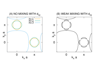
Figure S3: Fermi surfaces of the $3d_{xz}/3d_{yz}$ bands ($n=1,2$) and of the $3d_{xy}$ band ($n=3$), with and without weak mixing. The $3d_{xz}/3d_{yz}$ bands are identical to Fig. 5 in the paper, while the $3d_{xy}$ band is hole-type and relatively flat, with nearest neighbor and next-nearest neighbor hopping parameters $t_{1}^{xy}=-40$ meV and $t_{2}^{xy}=-28$ meV. The splitting between the $3d_{xy}$ and the $3d_{xz}/3d_{yz}$ orbitals is set to $\Delta E=20$ meV. As in the paper, the momentum $(k_{x},k_{y})$ coincides with pseudo momentum. (See ref. S_Lee_Wen_08 and the text.)

And what is the effect of the wavefunction renormalization $Z$ of the $3d_{xz}/3d_{yz}$ bands on the $3d_{xy}$ band? To answer this question, let us first write the determinant of the matrix inverse (S6) as $|G^{-1}(\omega)|=Z^{2}(\omega-\omega_{1})(\omega-\omega_{2})(\omega-\omega_{3})$, where $\omega_{1}$, $\omega_{2}$, and $\omega_{3}$ are the three roots of the charactersistic equation $|G^{-1}(\omega)|=0$. Near the Fermi surface of the $3d_{xy}$ band shown by Fig. S3b, $\omega_{3}({\bm{k}})=0$, the former determinant can therefore be approximated by $|G^{-1}(\omega)|=A_{3}(\omega-\omega_{3})$, with a constant prefactor

$$A_{3}={\partial\over{\partial\omega}}|G^{-1}|_{3}=3a_{3}\omega_{3}^{2}+2a_{2}\omega_{3}+a_{1}=a_{1}.$$ (S16)

Yet the determinant of the $2\times 2$ minor matrix $g^{-1}(3,3)$ of (S6) is

$$|g^{-1}(3,3)|=[Z\omega-(\varepsilon_{-}+\nu)][Z\omega-(\varepsilon_{+}-\nu)].$$ (S17)

Cramer’s Rule (S7) thereby yields the following diagonal component for the electron propagator in the $3d_{xy}$ band near the Fermi surface, $\omega_{3}({\bm{k}})=0$:

$$G_{3,3}(\omega)={Z_{3}^{-1}\over{\omega-\omega_{3}}}\quad{\rm with}\quad Z_{3}={a_{1}\over{(\varepsilon_{-}+\nu)(\varepsilon_{+}-\nu)}}.$$ (S18)

Last, the characteristic equation at the Fermi surface is equivalent to $a_{0}=0$. Study of the expression (S14d) for the coefficient $a_{0}$ yields the identity

$$\varepsilon_{xy}+\Delta E={|\varepsilon_{y(\delta)z,xy}|^{2}\over{\varepsilon_{-}+\nu}}+{|\varepsilon_{x(\delta)z,xy}|^{2}\over{\varepsilon_{+}-\nu}}.$$ (S19)

After substituting it into the expression (S14c) for the coefficient $a_{1}$, (S18) then ultimately yields the following result for the inherited wavefunction renormalization:

$$Z_{3}=1+\biggl{[}{|\varepsilon_{y(\delta)z,xy}|^{2}\over{(\varepsilon_{-}+\nu)^{2}}}+{|\varepsilon_{x(\delta)z,xy}|^{2}\over{(\varepsilon_{+}-\nu)^{2}}}\biggr{]}Z.$$ (S20)

The $3d_{xy}$ band therefore inherits the divergent wavefunction renormalization of the $3d_{xz}/3d_{yz}$ bands at the Fermi level, $\omega\rightarrow 0$: $Z\rightarrow\infty$ implies $Z_{3}\rightarrow\infty$.

And how do the above results depend on changes in the nature of the three Fermi surfaces in the absence of mixing with the $3d_{xy}$ orbital that are shown in Fig. S3a ? Increasing the size of the hole-type Fermi surface ($n=3$) for the $3d_{xy}$ electrons is achieved by increasing the energy splitting $\Delta E$ between the $3d_{xy}$ and $3d_{xz}/3d_{yz}$ orbitals, while increasing the size of the electron/hole Fermi surface pockets ($n=1,2$) for the $3d_{xz}/3d_{yz}$ electrons is achieved by lowering the on-site repulsive energy $U(\pi)$. [See Eq. (49) in the paper.] Either of these changes in parameters can result in $3d_{xy}$ orbital character at the tips of the electron Fermi surface pockets, $n=1$. (Cf. Fig. S3a.) It coincides with predictions made by band-structure calculations in the case of alkali-metal intercalated iron selenidesS_maier_11 ; S_mazin_11 .

Appendix C Spin-Orbit Coupling

Consider next adding spin-orbit coupling at each iron atom:

$$H_{\rm SO}=\lambda_{\rm SO}{\bm{L}}\cdot{\bm{S}}=\lambda_{\rm SO}\Bigl{(}{1\over 2}L_{+}S_{-}+{1\over 2}L_{-}S_{+}+L_{z}S_{z}\Bigr{)}.$$ (S21)

The principal iron orbitals at the electron Fermi surface pockets in FeSe are the degenerate $3d_{xz}/3d_{yz}$ orbitals and the $3d_{xy}$ orbital. Henceforth, we therefore shall project out the $3d_{x^{2}-y^{2}}$ and the $3d_{2z^{2}-x^{2}-y^{2}}$ orbitalsS_agterberg_17 ; S_eugenio_vafek_18 . Two irreducible Hilbert spaces thereby emerge under the spin-orbit Hamiltonian (S21):

$$\{|d_{y(\delta)z},\uparrow\rangle,|d_{x(\delta)z},\uparrow\rangle,|d_{xy},\downarrow\rangle\}\quad{\rm and}\quad\{|d_{y(\delta)z},\downarrow\rangle,|d_{x(\delta)z},\downarrow\rangle,|d_{xy},\uparrow\rangle\}.$$ (S22)

Above, $x(\delta)$ and $y(\delta)$ are the orbital coordinates measured with respect to new axes rotated by an angle $-\delta$ about the $z$ axis. Matrix elements of $H_{\rm SO}$ between the two Hilbert spaces above are null. On the other hand, matrix elements of $H_{\rm SO}$ within each one of the two Hilbert spaces above are easily computed, and these are listed in Tables 1 and 2.

$\langle m|H_{\rm SO}|n\rangle$	$|d_{y(\delta)z},\uparrow\rangle$	$|d_{x(\delta)z},\uparrow\rangle$	$|d_{xy},\downarrow\rangle$
$\langle d_{y(\delta)z},\uparrow|$	$0$	$+i\lambda_{\rm SO}/2$	$-e^{-i\delta}\lambda_{\rm SO}/2$
$\langle d_{x(\delta)z},\uparrow|$	$-i\lambda_{\rm SO}/2$	$0$	$+ie^{-i\delta}\lambda_{\rm SO}/2$
$\langle d_{xy},\downarrow|$	$-e^{+i\delta}\lambda_{\rm SO}/2$	$-ie^{+i\delta}\lambda_{\rm SO}/2$	$0$

Table 1: Matrix elements for spin-orbit coupling, Eq. (S21), in the “up” irreducible Hilbert space. See Eq. (S22).

$\langle m|H_{\rm SO}|n\rangle$	$|d_{y(\delta)z},\downarrow\rangle$	$|d_{x(\delta)z},\downarrow\rangle$	$|d_{xy},\uparrow\rangle$
$\langle d_{y(\delta)z},\downarrow|$	$0$	$-i\lambda_{\rm SO}/2$	$+e^{+i\delta}\lambda_{\rm SO}/2$
$\langle d_{x(\delta)z},\downarrow|$	$+i\lambda_{\rm SO}/2$	$0$	$+ie^{+i\delta}\lambda_{\rm SO}/2$
$\langle d_{xy},\uparrow|$	$+e^{-i\delta}\lambda_{\rm SO}/2$	$-ie^{-i\delta}\lambda_{\rm SO}/2$	$0$

Table 2: Matrix elements for spin-orbit coupling, Eq. (S21), in the “down” irreducible Hilbert space. See Eq. (S22).

In the previous sections, all momentum quantum numbers $\bm{k}$ coincide with pseudo momentumS_Lee_Wen_08 ${\bm{\tilde{k}}}$. Specifically, plane waves within the tight-binding approximation have the form (S1). Yet does pseudo momentum remain a good quantum number when the spin-orbit interaction (S21) at each iron atom is included? Observe that $P_{z}^{-1}L_{x}P_{z}=-L_{x}$, that $P_{z}^{-1}L_{y}P_{z}=-L_{y}$, and that $P_{z}^{-1}L_{z}P_{z}=+L_{z}$. Angular momentum then does not commute with a reflection about the $x$-$y$ plane, hence pseudo momentum is no longer a good quantum number when the spin-orbit interaction (S21) is included.

The square lattice of spin-orbit interactions (S21) does, however, commute with $T(a{\bm{\hat{x}}})$ and with $T(a{\bm{\hat{y}}})$. This means that conventional crystal momentum ${\bm{k}}$ remains a good quantum number, with conventional tight-binding plane waves

$$|{\bm{k}},\alpha\rangle\rangle=N_{\rm Fe}^{-1/2}\sum_{m,n}e^{i{\bm{k}}\cdot{\bm{R}}(m,n)}[T(a{\bm{\hat{x}}})]^{m}[T(a{\bm{\hat{y}}})]^{n}|\alpha\rangle.$$ (S23)

If we turn off the contribution due to electrostatic interactions to hopping between the $3d_{xz}/3d_{yz}$ orbitals and the $3d_{xy}$ orbital, $t_{xz,xy}=0=t_{yz,xy}$, then the on-site irreducible Hilbert spaces (S22) under the spin-orbit interaction can be extended to the following sets of plane-wave states:

$$\{|{\bm{k}},d_{y(\delta)z},\uparrow\rangle\rangle,|{\bm{k}},d_{x(\delta)z},\uparrow\rangle\rangle,|{\bm{k}},d_{xy},\downarrow\rangle\rangle\}\quad{\rm and}\quad\{|{\bm{k}},d_{y(\delta)z},\downarrow\rangle\rangle,|{\bm{k}},d_{x(\delta)z},\downarrow\rangle\rangle,|{\bm{k}},d_{xy},\uparrow\rangle\rangle\}.$$ (S24)

Observe, now, that $P_{z}|d_{x(\delta)z}\rangle=-|d_{x(\delta)z}\rangle$ and $P_{z}|d_{y(\delta)z}\rangle=-|d_{y(\delta)z}\rangle$ , while $P_{z}|d_{xy}\rangle=+|d_{xy}\rangle$. By (S1), this means that the conventional crystal momentum for electrons in the $3d_{xz}/3d_{yz}$ orbitals is shifted with respect to the pseudo momentum by the checkerboard wavenumber ${\bm{Q}}_{\rm AF}$, while that the conventional crystal momentum for electrons in the $3d_{xy}$ orbital coincides with the pseudo momentum. In conclusion, the inverse Greens function for the Eliashberg Theory in the paper, at null superconducting gaps, has the form

$$G^{-1}\cong\begin{bmatrix}Z\omega-(\varepsilon_{-}+\nu)&-\varepsilon_{y(\delta)z,x(\delta)z}&-\varepsilon_{y(\delta)z,xy}\\ -\varepsilon_{x(\delta)z,y(\delta)z}&Z\omega-(\varepsilon_{+}-\nu)&-\varepsilon_{x(\delta)z,xy}\\ -\varepsilon_{xy,y(\delta)z}&-\varepsilon_{xy,x(\delta)z}&\omega-{\bar{\varepsilon}}_{xy}-\Delta E\end{bmatrix},$$ (S25)

where ${\bar{\varepsilon}}_{xy}({\bm{k}})=\varepsilon_{xy}({\bm{k}}+{\bm{Q}}_{\rm AF})$, and where the off-diagonal matrix elements above, $\varepsilon_{\alpha,\beta}$, coincide with those for the spin-orbit interaction that are listed in Tables 1 and 2.

The determinant of the inverse Greens function (S25) is given by

$$|G^{-1}| = [Z\omega-(\varepsilon_{-}+\nu)][Z\omega-(\varepsilon_{+}-\nu)](\omega-{\bar{\varepsilon}}_{xy}-\Delta E)$$ (S26)

$$-|\varepsilon_{y(\delta)z,xy}|^{2}[Z\omega-(\varepsilon_{+}-\nu)]-|\varepsilon_{x(\delta)z,xy}|^{2}[Z\omega-(\varepsilon_{-}+\nu)]$$

$$-|\varepsilon_{y(\delta)z,x(\delta)z}|^{2}(\omega-{\bar{\varepsilon}}_{xy}-\Delta E)$$

$$-\varepsilon_{y(\delta)z,x(\delta)z}\varepsilon_{x(\delta)z,xy}\varepsilon_{xy,y(\delta)z}-\varepsilon_{x(\delta)z,y(\delta)z}\varepsilon_{y(\delta)z,xy}\varepsilon_{xy,x(\delta)z}.$$

Then by Cramer’s Rule (S7), the Greens functions among the $3d_{xz}/3d_{yz}$ orbitals are given by diagonal components $G_{1,1}\cong[Z\omega-(\varepsilon_{-}+\nu)]^{-1}$ and $G_{2,2}\cong[Z\omega-(\varepsilon_{+}-\nu)]^{-1}$, and by off-diagonal components $G_{1,2}\cong\varepsilon_{y(\delta)z,x(\delta)z}/([Z\omega-(\varepsilon_{-}+\nu)][Z\omega-(\varepsilon_{+}-\nu)])$ and $G_{2,1}=G_{1,2}^{*}$, up to first order in the spin-orbit coupling, $\lambda_{\rm SO}$. Substituting the latter into the off-diagonal self-energy corrections depicted by Fig. S2 yields that the portion of the spin-orbit interaction, $\lambda_{\rm SO}L_{z}S_{z}$, that is represented by the off-diagonal matrix elements $\varepsilon_{x(\delta)z,y(\delta)z}$ and $\varepsilon_{y(\delta)z,x(\delta)z}$ receives substantial renormalization within Eliashberg Theory. On the other hand, substitution of the former into Fig. S2 suggests that the divergent wave function renormalization and the Lifshitz transition that are predicted in the absence of the $3d_{xy}$ orbital by Eliashberg Theory survive the addition of the $3d_{xy}$ orbital and of the spin-orbit interaction.

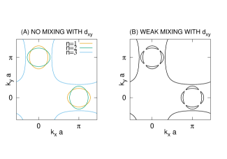
Figure S4: Fermi surfaces of the $3d_{xz}/3d_{yz}$ bands ($n=1,2$) and of the $3d_{xy}$ band ($n=3$), weakly mixing via the spin-orbit interactions at each iron atom. The $3d_{xz}/3d_{yz}$ bands are identical to those in Fig. 5 of the paper. Also, the $3d_{xy}$ band is identical to that in Fig. S3, but the momentum $(k_{x},k_{y})$ coincides with the crystal momentum shifted by the checkerboard wavevector $(\pi/a,\pi/a)$.

And as in the previous case of the background electrostatic potential, do the electrons at the Fermi surface of the $3d_{xy}$ band, $\omega_{3}({\bm{k}})$, inherit the infinite wavefunction renormalization from the $3d_{xz}/3d_{yz}$ bands at the Fermi surface at half filling? To answer this question, we first expand the expression above for the determinant (S26). This yields the third-order polynomial (S13), with coefficients that are given by

$$a_{3}= Z^{2},$$ (S27a)

$$a_{2}= -({\bar{\varepsilon}}_{xy}+\Delta E)Z^{2}-(\varepsilon_{+}+\varepsilon_{-})Z,$$ (S27b)

$$a_{1}= ({\bar{\varepsilon}}_{xy}+\Delta E)(\varepsilon_{+}+\varepsilon_{-})Z-(|\varepsilon_{y(\delta)z,xy}|^{2}+|\varepsilon_{x(\delta)z,xy}|^{2})Z$$

$$-|\varepsilon_{y(\delta)z,x(\delta)z}|^{2}+(\varepsilon_{-}+\nu)(\varepsilon_{+}-\nu),$$ (S27c)

$$a_{0}= -(\varepsilon_{-}+\nu)(\varepsilon_{+}-\nu)({\bar{\varepsilon}}_{xy}+\Delta E)+(\varepsilon_{+}-\nu)|\varepsilon_{y(\delta)z,xy}|^{2}+(\varepsilon_{-}+\nu)|\varepsilon_{x(\delta)z,xy}|^{2}$$

$$+({\bar{\varepsilon}}_{xy}+\Delta E)|\varepsilon_{y(\delta)z,x(\delta)z}|^{2}-\varepsilon_{y(\delta)z,x(\delta)z}\varepsilon_{x(\delta)z,xy}\varepsilon_{xy,y(\delta)z}-\varepsilon_{x(\delta)z,y(\delta)z}\varepsilon_{y(\delta)z,xy}\varepsilon_{xy,x(\delta)z}.$$ (S27d)

The off-diagonal matrix elements above, $\varepsilon_{\alpha,\beta}$, are listed in Tables 1 and 2. Following the previous analysis (S16), the determinant at frequencies $\omega$ approaching the Fermi surface, $\omega_{3}({\bm{k}})=0$, is given by $|G^{-1}(\omega)|=a_{1}(\omega-\omega_{3})$. And in the present case, the $2\times 2$ minor matrix $g^{-1}(3,3)$ has determinant

$$|g^{-1}(3,3)|=[Z\omega-(\varepsilon_{-}+\nu)][Z\omega-(\varepsilon_{+}-\nu)]-|\varepsilon_{y(\delta)z,x(\delta)z}|^{2}.$$ (S28)

By Cramer’s Rule (S7), the wavefunction renormalization at the Fermi surface for $3d_{xy}$ electrons is then

$$Z_{3}={a_{1}\over{(\varepsilon_{-}+\nu)(\varepsilon_{+}-\nu)-|\varepsilon_{y(\delta)z,x(\delta)z}|^{2}}}.$$ (S29)

Now recall that the Fermi surface is determined by the characteristic equation $a_{0}=0$. Using expression (S27) for the coefficient $a_{0}$ thereby yields the identity (S19) to lowest non-trivial order in the mixing with the $3d_{xy}$ orbital, with the exception that $\varepsilon_{xy}$ is replaced by ${\bar{\varepsilon}}_{xy}$. After substituting it into expression (S27) for the coefficient $a_{1}$, (S29) in turn yields expression (S20) for the wavefunction renormalization at weak mixing with the $3d_{xy}$ orbital, in the regime of large wavefunction renormalization, $Z\gg 1$. The wavefunction renormalization $Z_{3}^{-1}$ is therefore positive, and it vanishes as $Z\rightarrow\infty$.

Figure S4b shows the Fermi surfaces set by the characteristic equation $|G^{-1}|=0$ at $\omega=0$; i.e., $a_{0}({\bm{k}})=0$. The $3d_{xz}/3d_{yz}$ and $3d_{xy}$ bands in isolation are identical to those shown by Fig. S3a, but the momentum $(k_{x},k_{y})$ instead coincides with the crystal momentum shifted by the checkerboard wavevector $(\pi/a,\pi/a)$. Here, the spin-orbit coupling energy is set to $\lambda_{\rm SO}=14$ meV. Notice the expected level repulsion shown by the $3d_{xz}/3d_{yz}$ Fermi surface pockets at $(\pi/a,0)$ and $(0,\pi/a)$ in Fig. S4b. The electronic filling fraction is close to half filling.

References

- (1) T. Qian, X.-P. Wang, W.-C. Jin, P. Zhang, P. Richard, G. Xu, X. Dai, Z. Fang, J.-G. Guo, X.-L. Chen, H. Ding, “Absence of a Holelike Fermi Surface for the Iron-Based K0.8Fe1.7Se2 Superconductor Revealed by Angle-Resolved Photoemission Spectroscopy”, Phys. Rev. Lett. 106, 187001 (2011).
- (2) M. Xu, Q. Q. Ge, R. Peng, Z. R. Ye, Juan Jiang, F. Chen, X. P. Shen, B. P. Xie, Y. Zhang, A. F. Wang, X. F. Wang, X. H. Chen, and D. L. Feng, “Evidence for an S-Wave Superconducting Gap in KxFe2-ySe2 from Angle-Resolved Photoemission”, Phys. Rev. B 85, 220504(R) (2012).
- (3) B. Zeng, B. Shen, G. F. Chen, J. B. He, D. M. Wang, C. H. Li, and H. H. Wen, “Nodeless Superconductivity of Single-Crystalline KxFe2-ySe2 Revealed by the Low-Temperature Specific Heat”, Phys. Rev. B 83, 144511 (2011).
- (4) Weiqiang Yu, L. Ma, J. B. He, D. M. Wang, T.-L. Xia, G. F. Chen, and Wei Bao, “77Se NMR Study of the Pairing Symmetry and the Spin Dynamics in KyFe2-xSe2”, Phys. Rev. Lett. 106, 197001 (2011).
- (5) Q.-Y. Wang, Z. Li, W.-H. Zhang, Z.-C. Zhang, J.-S. Zhang, W. Li, H. Ding, Y.-B. Ou, P. Deng, K. Chang, J. Wen, C.-L. Song, K. He, J.-F. Jia, S.-H. Ji, Y. Wang, L. Wang, X. Chen, X. Ma, Q.-K. Xue, “Interface-Induced High-Temperature Superconductivity in Single Unit-Cell FeSe Films on SrTiO3”, Chin. Phys. Lett. 29, 037402 (2012).
- (6) W.-H. Zhang, Y. Sun, J.-S. Zhang, F.-S. Li, M.-H. Guo, Y.-F. Zhao, H.-M. Zhang, J.-P. Peng, Y. Xing, H.-C. Wang, T. Fujita, A. Hirata, Z. Li, H. Ding, C.-J. Tang, M. Wang, Q.-Y. Wang, K. He, S.-H. Ji, X. Chen, J.-F. Wang, Z.-C. Xia, L. Li, Y.-Y. Wang, J. Wang, L.-L. Wang, M.-W. Chen, Q.-K. Xue, and X.-C. Ma, “Direct Observation of High-Temperature Superconductivity in One-Unit-Cell FeSe Films”, Chin. Phys. Lett. 31, 017401 (2014).
- (7) L.Z. Deng, B. Lv, Z. Wu, Y.Y. Xue, W.H. Zhang, F.S. Li, L.L. Wang, X.C. Ma, Q.K. Xue, and C.W. Chu, “Meissner and Mesoscopic Superconducting States in 1–4 Unit-Cell FeSe Films”, Phys. Rev. B 90, 214513 (2014).
- (8) J.-F. Ge, Z.-L. Liu, C. Liu, C.-L. Gao, D. Qian, Q.-K. Xue, Y. Liu, J.-F. Jia, “Superconductivity Above 100 K in Single-Layer FeSe Films on Doped SrTiO3”, Nat. Mater. 14, 285 (2015).
- (9) D. Liu, W. Zhang, D. Mou, J. He, Y.-B. Ou,Q.-Y. Wang, Z. Li, L. Wang, L. Zhao, S. He, Y. Peng, X. Liu, C. Chaoyu, L. Yu, G. Liu, X. Dong, J. Zhang, C. Chen, Z. Xu, J. Hu, X. Chen, Z. Ma, Q. Xue and X.J. Zhou, “Electronic Origin of High-Temperature Superconductivity in Single-Layer FeSe Superconductor”, Nat. Comm. 3, 931 (2012).
- (10) R. Peng, X.P. Shen, X. Xie, H.C. Xu, S.Y. Tan, M. Xia, T. Zhang, H.Y. Cao, X.G. Gong, J.P. Hu, B.P. Xie, D. L. Feng, “Measurement of an Enhanced Superconducting Phase and a Pronounced Anisotropy of the Energy Gap of a Strained FeSe Single Layer in FeSe/Nb: SrTiO3/KTaO3 Heterostructures Using Photoemission Spectroscopy”, Phys. Rev. Lett. 112, 107001 (2014).
- (11) J.J. Lee, F.T. Schmitt, R.G. Moore, S. Johnston, Y.-T. Cui, W. Li, M. Yi, Z.K. Liu, M. Hashimoto, Y. Zhang, D.H. Lu, T.P. Devereaux, D.-H. Lee and Z.-X. Shen, “Interfacial Mode Coupling as the Origin of the Enhancement of in FeSe Films on SrTiO3”, Nature 515, 245 (2014).
- (12) Q. Fan, W.H. Zhang, X. Liu, Y.J. Yan, M.Q. Ren, R. Peng, H.C. Xu, B.P. Xie, J.P. Hu, T. Zhang, and D.L. Feng, “Plain S-Wave Superconductivity in Single-Layer FeSe on SrTiO3 Probed by Scanning Tunneling Microscopy”, Nat. Phys. 11, 946 (2015).
- (13) L. Zhao, A. Liang, D. Yuan, Y. Hu, D. Liu, J. Huang, S. He, B. Shen, Y. Xu, X. Liu, L. Yu, G. Liu, H. Zhou, Y. Huang, X. Dong, F. Zhou, Z. Zhao, C. Chen, Z. Xu, X.J. Zhou, “Common Electronic Origin of Superconductivity in (Li,Fe)OHFeSe Bulk Superconductor and Single-Layer FeSe/SrTiO3 Films”, Nat. Comm. 7, 10608 (2016).
- (14) X.H. Niu, R. Peng, H.C. Xu, Y.J. Yan, J. Jiang, D.F. Xu, T.L. Yu, Q. Song, Z.C. Huang, Y.X. Wang, B.P. Xie, X.F. Lu, N.Z. Wang, X.H. Chen, Z. Sun, and D.L. Feng, “Surface Electronic Structure and Isotropic Superconducting Gap in (Li0.8Fe0.2)OHFeSe”, Phys. Rev. B 92, 060504(R) (2015).
- (15) Y.J. Yan, W.H. Zhang, M.Q. Ren, X. Liu, X.F. Lu, N. Z. Wang, X.H. Niu, Q. Fan, J. Miao, R. Tao, B.P. Xie, X.H. Chen, T. Zhang, D.L. Feng, “Surface Electronic Structure and Evidence of Plain S-Wave Superconductivity in (Li0.8Fe0.2)OHFeSe”, Phys. Rev. B 94, 134502 (2016).
- (16) S.L. Bud’ko, M. Sturza, D.Y. Chung, M.G. Kanatzidis and P.C. Canfield, “Heat Capacity Jump at and Pressure Derivatives of Superconducting Transition Temperature in the Ba1-xKxFe2As2 () Series”, Phys. Rev. B 87, 100509(R) (2013).
- (17) T. Sato, K. Nakayama, Y. Sekiba, P. Richard, Y.-M. Xu, S. Souma, T. Takahashi, G.F. Chen, J.L. Luo, N.L. Wang and H. Ding, “Band Structure and Fermi Surface of an Extremely Overdoped Iron-Based Superconductor KFe2As2”, Phys. Rev. Lett. 103, 047002 (2009).
- (18) T.A. Maier, S. Graser, P.J. Hirschfeld, D.J. Scalapino, “D-Wave Pairing from Spin Fluctuations in the KxFe2-ySe2 Superconductors”, Phys. Rev. B 83, 100515(R) (2011).
- (19) F. Wang, F. Yang, M. Gao, Z.-Y. Lu, T. Xiang, D.-H. Lee, “The Electron Pairing of KxFe2-ySe2”, Europhys. Lett. 93, 57003 (2011).
- (20) I.I. Mazin, “Symmetry Analysis of Possible Superconducting States in KxFeySe2 Superconductors”, Phys. Rev. B 84, 024529 (2011).
- (21) P.A. Lee and X.-G. Wen, “Spin-Triplet P-Wave Pairing in a Three-Orbital Model for Iron Pnictide Superconductors”, Phys. Rev. B 78, 144517 (2008).
- (22) D.F. Agterberg, T. Shishidou, J. O’Halloran, P.M.R. Brydon, and M. Weinert, “Resilient Nodeless D-Wave Superconductivity in Monolayer FeSe”, Phys. Rev. Lett. 119, 267001 (2017).
- (23) P.M. Eugenio and O. Vafek, “Classification of Symmetry Derived Pairing at the M Point in FeSe”, Phys. Rev. B 98, 014503 (2018).
- (24) M. Khodas and A.V. Chubukov, “Interpocket Pairing and Gap Symmetry in Fe-Based Superconductors with Only Electron Pockets”, Phys. Rev. Lett. 108, 247003 (2012).
- (25) E. Berg, M.A. Metlitski and S. Sachdev, “Sign-Problem-Free Quantum Monte Carlo of the Onset of Antiferromagnetism in Metals”, Science 338, 1606 (2012).
- (26) J.P. Rodriguez and R. Melendrez, “Fermi Surface Pockets in Electron-Doped Iron Superconductor by Lifshitz Transition”, J. Phys. Commun. 2, 105011 (2018); “Corrigendum: Fermi Surface Pockets in Electron-Doped Iron Superconductor by Lifshitz Transition”, J. Phys. Commun. 3, 019501 (2019).
- (27) C. Xu, M. Müller, and S. Sachdev, “Ising and Spin Orders in the Iron-Based Superconductors”, Phys. Rev. B 78, 020501(R) (2008).
- (28) J. Kang and R.M. Fernandes, “Superconductivity in FeSe Thin Films Driven by the Interplay between Nematic Fluctuations and Spin-Orbit Coupling”, Phys. Rev. Lett. 117, 217003 (2016).
- (29) J.P. Rodriguez, “Isotropic Cooper Pairs with Emergent Sign Changes in a Single-Layer Iron Superconductor”, Phys. Rev. B 95, 134511 (2017).
- (30) S. Raghu, Xiao-Liang Qi, Chao-Xing Liu, D.J. Scalapino, Shou-Cheng Zhang, “Minimal Two-Band Model of the Superconducting Iron Oxypnictides”, Phys. Rev. B 77, 220503(R) (2008).
- (31) J.P. Rodriguez, M.A.N. Araujo, P.D. Sacramento, “Emergent Nesting of the Fermi Surface from Local-Moment Description of Iron-Pnictide High- Superconductors”, Eur. Phys. J. B 87, 163 (2014).
- (32) M. Daghofer, A. Moreo, J.A. Riera, E. Arrigoni, D.J. Scalapino, and E. Dagotto, “Model for the Magnetic Order and Pairing Channels in Fe Pnictide Superconductors”, Phys. Rev. Lett. 101, 237004 (2008); A. Moreo, M. Daghofer, J.A. Riera, and E. Dagotto, “Properties of a Two-Orbital Model for Oxypnictide Superconductors: Magnetic Order, B2g Spin-Singlet Pairing Channel, and its Nodal Structure”, Phys. Rev. B 79, 134502 (2009).
- (33) P.S. Riseborough, B. Coqblin, S.G. Magalhães, “Phase Transition Arising from the Underscreened Anderson Lattice Model: A Candidate Concept for Explaining Hidden Order in URu2Si2”, Phys. Rev. B 85, 165116 (2012).
- (34) J.P. Rodriguez, “Magnetic Excitations in Ferropnictide Materials Controlled by a Quantum Critical Point into Hidden Order”, Phys. Rev. B 82, 014505 (2010).
- (35) P.W. Anderson, “An Approximate Quantum Theory of the Antiferromagnetic Ground State”, Phys. Rev. 86, 694 (1952).
- (36) B.I. Halperin and P.C. Hohenberg, “Hydrodynamic Theory of Spin Waves”, Phys. Rev. 188, 898 (1969).
- (37) D. Forster, Hydrodynamic Fluctuations, Broken Symmetry, and Correlation Functions (Benjamin/Cummings), Reading, MA, 1975).
- (38) J.P. Rodriguez, “Spin Resonances in Iron-Selenide High- Superconductors by Proximity to Hidden Spin Density Wave”, Phys. Rev. B 102, 024521 (2020).
- (39) G.M. Eliashberg, “Interactions between Electrons and Lattice Vibrations in a Superconductor”, Sov. Phys. JETP 11, 696 (1960).
- (40) G.M. Eliashberg, “Temperature Green’s Function for Electrons in a Superconductor”, Sov. Phys. JETP 12, 1000 (1961).
- (41) J.R. Schrieffer, Theory of Superconductivity (Benjamin, New York, 1964).
- (42) D.J. Scalapino, in Superconductivity, v. 1, ed. R.D. Parks (Dekker, New York, 1969).
- (43) Y. Nambu, “Quasi-Particles and Gauge Invariance in the Theory of Superconductivity”, Phys. Rev. 117, 648 (1960).
- (44) L.P. Gorkov, Zh. Eksperim. i Teor. Fiz. 34, 735 1958; “About the Energy Spectrum of Superconductors”, Sov. Phys. JETP 7, 505 (1958).
- (45) I.I. Mazin, D.J. Singh, M.D. Johannes, and M.H. Du, “Unconventional Superconductivity with a Sign Reversal in the Order Parameter of LaFeAsO1-xFx”, Phys. Rev. Lett. 101, 057003 (2008).
- (46) K. Kuroki, S. Onari, R. Arita, H. Usui, Y. Tanaka, H. Kontani, and H. Aoki, “Unconventional Pairing Originating from the Disconnected Fermi Surfaces of Superconducting LaFeAsO1-xFx”, Phys. Rev. Lett. 101, 087004 (2008).
- (47) S. Graser, T.A. Maier, P.J. Hirschfeld, and D.J. Scalapino, “Near-Degeneracy of Several Pairing Channels in Multiorbital Models for the Fe Pnictides”, New J. Phys. 11, 025016 (2009).
- (48) A. Linscheid, S. Maiti, Y. Wang, S. Johnston, and P.J. Hirschfeld, “High- via Spin Fluctuations from Incipient Bands: Application to Monolayers and Intercalates of FeSe”, Phys. Rev. Lett. 117, 077003 (2016).
- (49) P. Morel and P.W. Anderson, “Calculation of the Superconducting State Parameters with Retarded Electron-Phonon Interaction”, Phys. Rev. 125, 1263 (1962).
- (50) W.L. McMillan, “Transition Temperature of Strong-Coupled Superconductors”, Phys. Rev. 167, 331 (1968).
- (51) High-Temperature Superconductivity, edited by V.L. Ginzburg and D.A. Kirzhnits (Consultants Bureau, New York, 1982).
- (52) J.P. Carbotte, “Properties of Boson-Exchange Superconductors”, Rev. Mod. Phys. 62, 1027 (1990).
- (53) B. Pan, Y. Shen, D. Hu, Y. Feng, J.T. Park, A.D. Christianson, Q. Wang, Y. Hao, H. Wo, Z. Yin, T.A. Maier and J. Zhao, “Structure of Spin Excitations in Heavily Electron-Doped Li0.8Fe0.2ODFeSe Superconductors”, Nat. Commun. 8, 123 (2017).
- (54) M. Yi, Z-K Liu, Y. Zhang, R. Yu, J.-X. Zhu, J.J. Lee, R.G. Moore, F.T. Schmitt, W. Li, S.C. Riggs, J.-H. Chu, B. Lv, J. Hu, M. Hashimoto, S.-K. Mo, Z. Hussain, Z.Q. Mao, C.W. Chu, I.R. Fisher, Q. Si, Z.-X. Shen, and D.H. Lu, “Observation of Universal Strong Orbital-Dependent Correlation Effects in Iron Chalcogenides”, Nat. Comm. 6, 7777 (2015).
- (55) R. Yu and Q. Si, “Orbital-Selective Mott Phase in Multiorbital Models for Alkaline Iron Selenides K1-xFe2-ySe2”, Phys. Rev. Lett. 110, 146402 (2013).
- (56) See Supplemental Material: I. Add Orbital to Eliashberg Theory with Orbitals; II. Effects and Properties of Orbital; III. Spin-Orbit Coupling.
- (57) O.V. Dolgov, I.I. Mazin, D. Parker, A.A. Golubov, “Interband Superconductivity: Contrasts between BCS and Eliashberg Theory”, Phys. Rev. B79, 060502(R) (2009); O.V. Dolgov, I.I. Mazin, D. Parker, A.A. Golubov, “Erratum: Interband Superconductivity: Contrasts between Bardeen-Cooper-Schrieffer and Eliashberg Theories [Phys. Rev. B 79, 060502(R) (2009)]”, Phys. Rev. B 80, 219901(E) (2009).
- (58) L. Benfatto, E. Cappelluti, and C. Castellani, “Spectroscopic and Thermodynamic Properties in a Four-Band Model for Pnictides”, Phys. Rev. B 80, 214522 (2009).
- (59) G. A. Ummarino, M. Tortello, D. Daghero, and R. S. Gonnelli “Three-Band s Eliashberg Theory and the Superconducting Gaps of Iron Pnictides” Phys. Rev. B 80, 172503 (2009).

References

- (1) P.A. Lee and X.-G. Wen, “Spin-Triplet P-Wave Pairing in a Three-Orbital Model for Iron Pnictide Superconductors”, Phys. Rev. B 78, 144517 (2008).
- (2) T.A. Maier, S. Graser, P.J. Hirschfeld, D.J. Scalapino, “D-Wave Pairing from Spin Fluctuations in the KxFe2-ySe2 Superconductors”, Phys. Rev. B 83, 100515(R) (2011).
- (3) I.I. Mazin, “Symmetry Analysis of Possible Superconducting States in KxFeySe2 Superconductors”, Phys. Rev. B 84, 024529 (2011).
- (4) D.F. Agterberg, T. Shishidou, J. O’Halloran, P.M.R. Brydon, and M. Weinert, “Resilient Nodeless D-Wave Superconductivity in Monolayer FeSe”, Phys. Rev. Lett. 119, 267001 (2017).
- (5) P.M. Eugenio and O. Vafek, “Classification of Symmetry Derived Pairing at the M Point in FeSe”, Phys. Rev. B 98, 014503 (2018).