Estimating the Unruh effect via entangled many-body probes

Abstract

We study the estimation of parameters in a quantum metrology scheme based on entangled many-body Unruh-DeWitt detectors. It is found that the precision for the estimation of Unruh effect can be enhanced via initial state preparations and parameter selections. It is shown that the precision in the estimation of the Unruh temperature in terms of a many-body-probe metrology is always better than the precision in two probe strategies. The proper acceleration for Bob’s detector and the interaction between the accelerated detector and the external field have significant influences on the precision for the Unruh effect’s estimation. In addition, the probe state prepared with more excited atoms in the initial state is found to perform better than less excited initial states. However, different from the estimation of the Unruh temperature, the estimation of the effective coupling parameter for the accelerated detector requires more total atoms but less excited atoms in the estimations.

I introduction

As predicted by quantum field theory in curved spacetime, quantum fluctuation will produce a local change in energy of an Unruh-DeWitt detector UW84 . It was found that the detectors will be thermalized at a temperature defined by some characteristic inverse length scale of the spacetime or motion through them, e.g. acceleration Matsas01 ; Unruh ; Unruhr , surface gravity Hawking74 , or Hubble constant Hawking77 . The feature that all three of these effects have in common is the existence of an event horizon. The detector will observe a radiation originating from quantum fluctuations near the horizon. The Unruh effect Matsas01 ; Unruh ; Unruhr predicts the thermality of a uniformly accelerated detector in the Minkowski vacuum. This thermality can be demonstrated by tracing the field modes beyond the Rindler event horizon therefore manifests itself as a decoherence-like effect. The Unruh-Hawking effect also makes a deep connection between black hole thermodynamics and quantum physics, such as the understanding of entanglement entropy and quantum nonlocality in curved spacetime.

Despite its crucial role in physics, the experimental detection of the Unruh effect is an open program on date. The main technical obstacle is that the Unruh temperature is smaller than 1 Kelvin even for accelerations up to $10^{21}m/s^{2}$ unruhreview . This means the detectable Unruh temperature lies far below the observable threshold with the experimentally achievable acceleration. Since experimental detection of the Unruh radiation is too difficult, people turn sight to the easier but still conceptually rich studies on the simulation natureobhawking and estimation of this effect. We know that quantum metrology aims to improve the precision in estimating parameters via quantum strategies Giovannetti2011 . The estimation is based on measurements made on a probe system that undergoes an evolution depending on the estimated parameters. Recently, quantum metrology has been applied to enhance the detection of gravitational wave beyond the standard quantum limit Abbott , the exploration of the Earth’s Schwarzschild parameters DEB ; wangmetro ; earthmetro , and the estimation of cosmological parameters in expanding universe wangmetro2 ; xiaobao . In particular, researchers found that quantum strategies can be employed to enhance the estimation of the Unruh-Hawking effect, both for accelerated free modes aspachs ; HoslerKok2013 ; RQI6 ; wangmetro3 ; unruhEPJC , local modes in moving cavities RQM ; RQM2 , and accelerated detectors wangmetro1 ; unruhJHEP2 ; unruhJHEPun1 . However, it is worthy of note that all probe states in the above-mentioned quantum enhanced estimation tasks for the Unruh-Hawking effect are prepared in bipartite entangled states.

In this paper, we employ a multipartite entangled probe strategy to estimate the Unruh temperature and related parameters. The probes for the quantum metrology are prepared by $n$ entangled Unruh-DeWitt detectors. Each detector is modeled by a two-level atom which interacts only with the neighbor field in the Minkowski vacuum UW84 . We assume that the second atom of multiparty system, carried by Bob, moves with constant acceleration and interacts with a massless scalar field while other atoms keep stationary. To analyze the maximum achievable precision in the estimation of the parameters, we calculate quantum Fisher information with respect to them. It is worth mentioning that, like the quantum Fisher information, the Wigner-Yanase-Dyson skew information skewinfor is also a variant of the Fisher information in the quantum regime. The latter is related to the quantum Hellinger distance Luo04 and has been shown to satisfy some nice properties relevant to quantum coherence Yadin16 ; unruhEPJC . Recently, the authors of unruhEPJC developed a Bloch vector representation of the Unruh channel and made a comparative study on the quantum Fisher and Skew information for free Dirac field modes. In this paper we only study the quantum Fisher information because the quantum Fisher and Skew information are in fact two different aspects of the classical Fisher information in the quantum regime Petz .

The outline of the paper is organized as follows. In Section. II, the evolution of the multiparty system is presented where one of the detectors travels with uniform acceleration. In Sec. III, we start with introducing some key concepts for quantum metrology especially the quantum Fisher information. Then we analyze the quantum Fisher information for estimating Unruh temperature $T$ and the effective coupling parameter $\nu$. The Sec. IV is devoted to a brief summary.

II The evolution of multiparty quantum system with an accelerated atom

In this section, we briefly introduce the dynamics of the multiparty entangled Unruh-DeWitt detectors. Assuming that the probe system consists of $n$ atoms, the initial state is prepared in a symmetric $Z$-type multipartite state Ben-Av ; Lizhang

$$|\psi_{t_{0}}\rangle = \sqrt{\frac{(n-k)!k!}{n!}}(|111...000\rangle$$ (1)

$$+ |11...01...00\rangle+...+|000...111\rangle),$$

where $k$ atoms own the excited energy eigenstate $|1\rangle$, while the rest $n-k$ atoms lie in the ground state $|0\rangle$. If $k=1$, it degenerates into a symmetric $W$-type state.

The total Hamiltonian of the entire probe system is

$$H_{n\phi}=\sum_{i=1}^{n}H_{i}+H_{KG}+H_{int}^{B\phi},$$ (2)

where $H_{KG}$ stands for the Hamiltonian of the massless scalar field satisfying the K-G equation $\Box\phi=0$. In Eq. (2), $H_{i}=\Omega D_{i}^{\dagger}D_{i},i=1,2...n$ are the Hamiltonian of each atom, where $D_{i}$ and $D_{i}^{\dagger}$ represent the creation and annihilation operators of the $i$th atom, respectively. We assume that the second atom of the multiparty system, carried by the observer Bob, is uniformly accelerated for a duration time $\Delta$, while other atoms keep static and have no interaction with the scalar field. The world line of Bob’s detector is given by

$$t(\tau)=a^{-1}\sinh a\tau,x(\tau)=a^{-1}\cosh a\tau,y(\tau)=z(\tau)=0,$$ (3)

where $a$ is the proper acceleration of Bob. The interaction Hamiltonian $H_{int}^{B\phi}$ between Bob’s detector and the field is Landulfo ; Landulfo1 ; wang3

$$H^{B\phi}_{int}(t)=\epsilon(t)\int_{\Sigma_{t}}d^{3}{\bf x}\sqrt{-g}\phi(x)[\chi({\bf x})D_{2}+\overline{\chi}({\bf x})D_{2}^{\dagger}],$$ (4)

where $\phi(x)$ is the scalar field operator, $\epsilon(t)$ is the coupling constant, $g_{ab}$ is the Minkowski metric and $g\equiv{\rm det}(g_{ab})$. In Eq. (4), $\Sigma_{t}$ represents the integration takes place over the global spacelike Cauchy surface. The function $\chi(\mathbf{x})$ vanishes outside a small volume around the detector, which describes that the detector only interacts with the neighbor field.

For convenience, introducing a compact support complex function $f(x)=\epsilon(t)e^{-i\Omega t}\chi({\bf x})$, we have $\phi(x)f\equiv Rf-Af$, where $A$ and $R$ are the advanced and retarded Green functions. Then one obtains Landulfo ; Landulfo1 ; wang3

$$\phi(f)\equiv\int d^{4}x\sqrt{-g}\phi(x)f=i[a_{RI}(\Gamma_{-}^{*})-a_{RI}^{\dagger}(\Gamma_{+})],$$ (5)

where $\Gamma_{-}$ and $\Gamma_{+}$ represent the negative and positive frequency parts of $\phi(f)$ respectively, and $a^{\dagger}_{RI}$ and $a_{RI}$ are Rindler creation and annihilation operators in region $I$ of Rindler spacetime. Since $\epsilon(t)$ is a roughly constant for $\Delta\gg\Omega^{-1}$, the test function $f$ approximately owns the positive-frequency part, which means $\Gamma_{-}\approx 0$. And if we define $\lambda\equiv-\Gamma_{+}$, Eq. (5) is found to be $\phi(f)\approx ia^{\dagger}(\lambda)$.

The whole initial state of $n$-party systems and the massless scalar field is $|\Psi_{t_{0}}^{n\phi}\rangle=|\psi_{t_{0}}\rangle\otimes|0\rangle_{M}$, where $|0\rangle_{M}$ stands for Minkowski vacuum. Here we only consider the first order under the weak-coupling limit. Using Eq. (4) and Eq. (5), we can calculate the final state of the probe state at time $t>t_{0}+\Delta$, which is

$$|\Psi_{t}^{n\phi}\rangle = T\exp[-i\int d^{4}x\sqrt{-g}\phi(x)(fD_{2}+\overline{f}D_{2}^{\dagger})]|\Psi_{t_{0}}^{n\phi}\rangle$$ (6)

$$\approx 1-i\int d^{4}x\sqrt{-g}\phi(x)[fD_{2}+\overline{f}D_{2}^{\dagger}]|\Psi_{t_{0}}^{n\phi}\rangle$$

$$= (1+a_{RI}^{\dagger}(\lambda)D_{2}-a_{RI}(\overline{\lambda})D_{2}^{\dagger})|\Psi_{t_{0}}^{n\phi}\rangle,$$

in the interaction picture, where $T$ is the time-order operator.

As discussed in Landulfo ; Landulfo1 ; wang3 ; wangmetro1 , the Bogliubov transformations between the operators of Minkowski modes and Rindler modes are

$$a_{RI}(\overline{\lambda}) = \frac{a_{M}(\overline{F_{1\Omega}})+e^{-\pi\Omega/a}a_{M}^{\dagger}(F_{2\Omega})}{(1-e^{-2\pi\Omega/a})^{{1}/{2}}},$$ (7)

$$a^{\dagger}_{RI}(\lambda) = \frac{a^{\dagger}_{M}(F_{1\Omega})+e^{-\pi\Omega/a}a_{M}(\overline{F_{2\Omega}})}{(1-e^{-2\pi\Omega/a})^{{1}/{2}}},$$ (8)

where $F_{1\Omega}=\frac{\lambda+e^{-\pi\Omega/a}\lambda\circ w}{(1-e^{-2\pi\Omega/a})^{{1}/{2}}}$, and $F_{2\Omega}=\frac{\overline{\lambda\circ w}+e^{-\pi\Omega/a}\overline{\lambda}}{(1-e^{-2\pi\Omega/a})^{{1}/{2}}}$. In $F_{1\Omega}$ and $F_{2\Omega}$, $w(t,x)=(-t,-x)$ denotes the wedge reflection isometry, which makes a reflection from $\lambda$ in Rindler region $I$ to $\lambda\circ w$ in Rindler region $II$.

By using the Bogliubov transformations given in Eqs. (7-8), Eq. (6) can be rewritten as

$$|\Psi_{t}^{n\phi}\rangle = |\Psi_{t_{0}}^{n\phi}\rangle+\frac{1}{(1-q)^{1/2}}\sqrt{\frac{(n-k)!k!}{n!}}(|\Psi_{1}^{n}\rangle$$ (9)

$$\otimes q^{1/2}|1_{F_{2\Omega}}\rangle+|\Psi_{2}^{n}\rangle\otimes|1_{F_{1\Omega}}\rangle\rangle),$$

where the parameterized acceleration $q\equiv e^{-2\pi\Omega/a}$ has been introduced. In Eq. (9),

$$|\Psi_{1}^{n}\rangle=(\underbrace{|11...00\rangle+...+|01...11\rangle}_{C_{n-1}^{k}\;\;terms}),$$ (10)

where Bob’s atom and $\frac{(n-1)!}{(n-k-1)!k!}$ atoms of the rest atoms are sure to lie in excited energy eigenstates $|1\rangle$.

$$|\Psi_{2}^{n}\rangle=(\underbrace{|10...00\rangle+...+|00...11\rangle}_{C_{n-1}^{k-1}\;\;terms}).$$ (11)

This means Bob’s atom is certain to be in ground state $|0\rangle$ and $\frac{(n-1)!}{(n-k)!(k-1)!}$ atoms in the rest atoms are sure to be involved in excited energy eigenstates.

Since we only concern about the probe state after the acceleration of Bob, the degrees of freedom of the external scalar field should be traced out. By doing this we obtain the final density matrix of the many-body probe system

$$\rho_{t}^{n} = |C|^{-2}\{|\psi_{t_{0}}\rangle\langle\psi_{t_{0}}|+\frac{n!}{(n-k)!k!}\frac{\nu^{2}}{1-q}$$ (12)

$$\times (q|\Psi_{1}^{n}\rangle\langle\Psi_{1}^{n}|+|\Psi_{2}^{n}\rangle\langle\Psi_{2}^{n}|)\},$$

with the energy gap $\Omega$ and the coupling constant $\epsilon$, where $\nu^{2}\equiv\frac{\epsilon^{2}\Omega\Delta}{2\pi}e^{-\Omega^{2}\kappa^{2}}$ is the effective coupling and $C=(1+\frac{q\nu^{2}(n-k)+\nu^{2}k}{(1-q)n})^{1/2}$ normalizes the final state $\rho_{t}^{n}$.

III Quantum metrology and quantum Fisher information for the Unruh effect

As an important quantity in the geometry of Hilbert spaces, the quantum Fisher information has a significant impact on quantum metrology, which evaluates the state sensitivity with the perturbation of the parameter Giovannetti2011 . For a statistic nature, the maximum achievable precision of quantum metrology is determined the quantum Cramér-Rao bound Cramer:Methods1946 , which demands a fundamental lower bound for the covariance matrix of the estimation Braunstein1994 ; Braunstein1996

$$Var(\epsilon)\geq\frac{1}{N\mathcal{F}_{\xi}(\epsilon)},$$ (13)

where $N$ is the number of measurements and $\mathcal{F}_{\xi}(\epsilon)$ is the Fisher information Braunstein1994 ; Braunstein1996

$$\mathcal{F}_{\xi}(\epsilon)=\int\mathcal{L}_{\epsilon}(\frac{\partial}{\partial\theta}\ln\ln L_{\epsilon})dx.$$ (14)

Here the symmetric logarithmic derivative (SLD) Hermitian operator $\mathcal{L}_{\epsilon}$ is defined as $\partial_{\epsilon}\,\rho_{\epsilon}=\frac{1}{2}\left\{\rho_{\epsilon},\mathcal{L}_{\epsilon}\right\}$, where $\partial_{\epsilon}\equiv\frac{\partial}{\partial\epsilon}$ and $\left\{\,\cdot\,,\,\cdot\,\right\}$ denotes the anticommutator. For any given POVM $\{\Pi_{\xi}\}$, Fisher information establish the bound on precision. To obtain the ultimate bounds on precision, one should maximize the Fisher information over all the possible measurements. Then we have Braunstein1994 ; Braunstein1996

$$\mathcal{F}_{\xi}(\epsilon) \leq\Sigma_{\xi}\left|\frac{Tr\left[\rho_{\epsilon}\Pi_{\xi}L_{T}\right]}{\sqrt{Tr[\rho_{\epsilon}\Pi_{\xi}]}}\right|^{2}$$

$$\leq\ \Sigma_{\xi}Tr\left[\Pi_{\xi}\mathcal{L}_{\epsilon}\rho_{\epsilon}\mathcal{L}_{\epsilon}\right]$$

$$=\mathcal{F}_{Q}(\epsilon),$$ (15)

where $\mathcal{F}_{Q}(\epsilon)$ is the quantum Fisher information Braunstein1994 ; Braunstein1996

$$\mathcal{F}_{Q}(\epsilon)=Tr[\partial_{\epsilon}\rho_{\epsilon}\mathcal{L}_{\epsilon}]=Tr[\rho_{\epsilon}\mathcal{L}_{\epsilon}^{2}].$$ (16)

Thus, optimizing over all the possible measurements leads to an lower quantum Cramér-Rao bound Braunstein1994 , i.e.,

$$Var(T)\geq\frac{1}{n\mathcal{F}_{\xi}(\epsilon)}\geq\frac{1}{n\mathcal{F}_{Q}(\epsilon)}.$$ (17)

By diagonalizing the density matrix as $\rho_{\epsilon}=\sum_{i=1}^{N}\lambda_{i}|\psi_{i}\rangle\langle\psi_{i}|$, the SLD operator $\mathcal{L}_{\epsilon}$ owns the form

$$\mathcal{L}_{\epsilon}=2\sum_{m,n}^{N}\frac{\langle\psi_{k}|\partial_{\epsilon}\rho_{\epsilon}|\psi_{k}\rangle}{\lambda_{m}+\lambda_{n}}|\psi_{n}\rangle\langle\psi_{m}|,$$ (18)

and the quantum Fisher information can be obtained by Zhong

$$\mathcal{F}_{Q}(\epsilon)=2\sum_{m,n}^{N}\frac{|\langle\psi_{m}|\partial_{\epsilon}\rho_{\epsilon}|\psi_{n}\rangle|^{2}}{\lambda_{m}+\lambda_{n}},$$ (19)

where the eigenvalues $\lambda_{i}\geq 0$ and $\sum_{i}^{N}\lambda_{i}=1$.

Then we calculate the quantum Fisher information of Unruh temperature $T$ for the final probe state to find the optimal choice to estimate the temperature. Obviously, the final density matrix Eq. (12) of the probe state is not full matrix because its rows with the basis $|000...000\rangle$ or $|111...111\rangle$ are zero. According to Eqs. (12) and (19), we can calculate the nonzero eigenvalues

$$\Gamma_{1} = \frac{(1-q)n}{(1-q)n+qv^{2}(n-k)+v^{2}k},$$

$$\Gamma_{2} = \frac{qv^{2}(n-k)}{(1-q)n+qv^{2}(n-k)+v^{2}k},$$

$$\Gamma_{3} = \frac{v^{2}k}{(1-q)n+qv^{2}(n-k)+v^{2}k}$$

as well as the quantum Fisher information of Unruh temperature $T$ for the final probe state. The quantum Fisher information is found to be

$$\mathcal{F}_{Q}(T)=\frac{\Omega^{2}qv^{2}[n^{2}-(1-q)k^{2}v^{2}+(1-q)kn(v^{2}-1)]}{(1-q)T^{4}[(1-q)kv^{2}+n(1-q+qv^{2})]^{2}}.$$ (20)

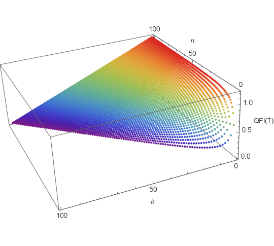
Figure 1: The quantum Fisher information for estimating Unruh temperature $T$ as functions of the total atoms $n$ and the excited atoms $k$ in the initial probe state Eq. (1). The energy gap $\Omega$, the acceleration $a$ and the effective coupling parameter $\nu$ are fixed as $\Omega=0.2$, $a=0.3$ and $\nu=0.1$, respectively.

In Fig. 1, we plot the quantum Fisher information for estimating the Unruh temperature $T$ as a function of the total atoms $n$ and the excited atoms $k$ in the initial probe state. In this model, the value of effective coupling parameter $\nu$ should be small enough to keep the perturbative approach valid for large times. It is shown that the amount of the total atoms $n$ and the excited atoms $k$ have significant influences on the value of quantum Fisher information. We find that the probe system owning the more total atoms would gain the higher quantum Fisher information. This means that the precision in the estimation of the Unruh temperature in terms of a many-body probe state is always better than precision in a bipartite probe system. That is to say, compared with previous bipartite metrology proposals, the multiparty-entangled-probe proposal for the quantum metrology of the Unruh effect is more workable and reliable. However, it is shown that with same atoms in the initial probe state, the less the excited atoms, the larger the quantum Fisher information. This means the number of excited atoms is disadvantage for the estimation of Unruh temperature. Therefore, the initial probe state prepared in $W$-type state always performs better than the $Z$-type probe state (if $k\neq 1$) for the same size initial state in the estimation of temperature $T$.

Figure 2: The quantum Fisher information for estimating the Unruh temperature $T$ as functions of the acceleration $a$ and the effective coupling parameter $\nu$. The total atoms $n$ and the excited atoms $k$ in the initial state of multiparty system are fixed as $n=3$ and $k=1$, respectively. The energy gap $\Omega$ is fixed as $\Omega=0.2$.

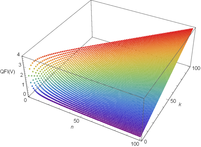
Figure 3: The quantum Fisher information for estimating the effective coupling parameter $\nu$ versus the total atoms $n$ and the excited atoms $k$ in the initial state of multiparty system. The energy gap $\Omega$, the acceleration $a$ and the effective coupling parameter $\nu$ are fixed as $\Omega=0.2$, $a=0.3$ and $\nu=0.1$, respectively.

In Fig. 2, the quantum Fisher information for estimating the Unruh temperature $T$ as functions of the acceleration $a$ and the effective coupling parameter $\nu$ is analyzed. It is show that the quantum Fisher information is not a monotonic increasing function of the acceleration $a$. Considering that a bigger quantum Fisher information corresponds to a higher precision, one can select a range of acceleration which provides better precision for the estimation of the Unruh temperature. Differently, as the effective coupling parameter $\nu$ increases, the quantum Fisher information for estimating the Unruh temperature increase. That is to say, the interaction between the atom and the scalar field would enhance the accuracy for estimating the Unruh temperature in the multiparty clock synchronization protocol.

We also interested in the estimation effective coupling parameter $\nu$ in the accelerated Unruh-DeWitt detectors. Employing the final state (12) the definition of quantum Fisher information (19), we can also calculate quantum Fisher information for the effective coupling parameter $\nu$. After some calculations, the quantum Fisher information for $\nu$ is found to be

$$\mathcal{F}_{Q}(v)=\frac{4n(1-q)[nq+(1-q)k]}{[(1-q)kv^{2}+n(1-q+qv^{2})]^{2}}.$$

In Fig. 3, we plot the quantum Fisher information for estimating the effective coupling parameter versus the total atoms $n$ and the excited atoms $k$ in the initial state of multiparty system. We find that, with more excited atoms in the same initial probe state, the precision for estimating the effective coupling parameter is higher. Different from the estimation of Unruh temperature, the estimation of the coupling parameter $\nu$ would gain more accuracy with the $Z$-type state (if $k\neq 1$) instead of the $W$-type state. But similar with the estimation of Unruh temperature, if the number of total atoms $n$ is smaller, the quantum Fisher information for estimating the coupling parameter would decrease, which means that a smaller multiparty system doesn’t support the estimation of the parameter $\nu$ in the many-body Unruh-DeWitt detector model.

In fact, the quantum Fisher information is a measure of macroscopic coherence because it can be demonstrated as the coherence of many copies of a state Yadin16 . The macroscopic coherence can be quantified by a superposition of states differing from one another in $A$-value by a fixed amount $\delta$. For the observable $A$, the quantum Fisher information can be expressed as Yadin16

$$\mathcal{F}_{Q}(\rho,A)=2\sum_{a,b}\frac{(\lambda_{a}-\lambda_{b})^{2}}{\lambda_{a}+\lambda_{b}}|\langle\psi_{a}|A|\psi_{b}\rangle|^{2},$$ (21)

where $\rho=\sum_{a}\lambda_{a}|\psi_{a}\rangle\langle\psi_{a}|$ is a spectral decomposition and the sum is over all $a,\,b$. For pure states, $\mathcal{F}_{Q}(|\psi\rangle\langle\psi|,A)=4V(|\psi\rangle,A)$, where $V(|\psi\rangle,A)=|\langle\psi_{a}|A^{2}|\psi_{b}\rangle|-|\langle\psi_{a}|A|\psi_{b}\rangle|^{2}$. For mixed states, assuming $|\psi\rangle$ is a reference state with $V(|\psi\rangle,A)=A_{0}$, the macroscopic coherence for $n$ copies can be defined via the observable $\sum_{i=1}^{n}A_{i}$. In the limit of large $n$, $|\psi\rangle^{\otimes n}$ and $|\psi\rangle^{\otimes m}$ have the same macroscopic coherence for all $\delta$, then we have $m/n=V(|\psi\rangle,A)/A_{0}$ Yadin16 . The minimal average ratio $m/n$ over all pure state decompositions $\rho=\sum_{\mu}p_{\mu}|\psi_{\mu}\rangle\langle\psi_{\mu}|$ is $\mathcal{F}_{Q}(\rho,A)/(4A_{0})$ Yadin16 . This means that the macroscopic coherence depends only on this distribution. If one take the reference state as a product of single-qubit states $\bigotimes_{i=1}^{N}|\phi_{i}\rangle$ with $V(|\phi_{i}\rangle,A_{i})=1$, the average ratio of copies is exactly $\mathcal{F}_{Q}(\rho,A)/(4N)$, where $\mathcal{F}_{Q}(\rho,A)$ is the quantum Fisher information for the ‘macroscopic observable’ $A$ and N is the number of qubits. That is to say, the quantum Fisher information can be employed to measure the maximum macroscopic coherence over all observables in $A$ Yadin16 . Therefore, the results of quantum Fisher information can in principle be used to understandin the behavior of macroscopic coherence embedded in the many detector system, which demands later study.

IV conclusions

In conclusion, we study the quantum Fisher information, a key concept in quantum metrology, in the estimation of Unruh temperature $T$ and the effective coupling parameter $\nu$ via an entangled many-body system. We find that the precision for the estimation of Unruh temperature in the multiparty entangled probe scheme performs better than the precision in two-party entangled probe systems. In addition, the precision of estimating Unruh effect would increase when the excited atoms become less in the probe state. It is shown that the proper acceleration for Bob’s detector and the interaction between the accelerated detector and the external field have significant influences on the precision for the Unruh effect’s estimation. To be specific, there are a range of proper accelerations that provide us witb a better precision in the estimation of the Unruh temperature. However, one should choose the largest effective coupling strength to achieve this goal. Alternatively, we can get a higher precision, i.e., a larger quantum Fisher information for a shorter interaction time and bigger the energy gaps. It is also found that, different from the estimation of Unruh temperature, it requires the $Z$-type initial state with more excited atoms for the estimation of the effective coupling parameter.

- (1) W. G. Unruh and R. M. Wald, Phys. Rev. D 29 (1984) 1047.
- (2) D. A. T. Vanzella and G. E. A. Matsas, Phys. Rev. Lett. 87 (2001) 151301.
- (3) W. G. Unruh, Phys. Rev. D 14 (1976) 870.
- (4) Luis C. B. Crispino, A. Higuchi, and George E. A. Matsas, Rev. Mod. Phys. 80, 787-838 (2008).
- (5) S. W. Hawking, Nature 248 (1974) 30.
- (6) G. W. Gibbons and S. W. Hawking, Phys. Rev.D 15 (1977) 2738.
- (7) Crispino, L. et al., Rev. Mod. Phys. 80 (2008) 787.
- (8) J. R. Munoz de Nova, K. Golubkov, V. I. Kolobov, J. Steinhauer, Nature 569 (2019) 688.
- (9) V. Giovannetti, S. Lloyd, and L. Maccone, Nat. Photon. 5 (2011) 222.
- (10) Y. Ma et.al., Nat. Phys. 13 (2017) 776.
- (11) D. E. Bruschi, A. Datta, R. Ursin, T. C. Ralph, and I. Fuentes, Phys. Rev. D, 90 (2014) 124001.
- (12) T. Liu, J. Jing, and J. Wang, Adv. Quantum Technol. 1 (2018) 1800072.
- (13) Sebastian P. Kish, and Timothy C. Ralph, Phys. Rev. D 99 (2019) 124015.
- (14) J. Wang, Z. Tian, J. Jing, and H. Fan, Nucl. Phys. B 892, (2015) 390; J. Wang, C. Wen, S. Chen, and J. Jing, Phys. Lett. B 800 (2020) 135109.
- (15) X. Liu, Z. Tian, J. Wang, and J. Jing, Eur. Phys. J. C 78 (2018) 665.
- (16) M. Aspachs, G. Adesso, and I. Fuentes, Phys. Rev. Lett. 105 (2010) 151301.
- (17) D. J. Hosler and P. Kok, Phys. Rev. A 88 (2013) 052112.
- (18) S. Banerjee, A. K. Alok, and S. Omkar, Eur. Phys. J. C 76 (2016) 437.
- (19) J. Wang, H. Cao, and J. Jing, Ann. Phys. 373 (2016) 188.
- (20) Y. Yao, X. Xiao, L. Ge, X. G. Wang, and C. P. Sun, Phys. Rev. A 89 (2014) 042336.
- (21) M. Ahmadi, D. E. Bruschi, N. Friis, C. Sabin, G. Adesso, and I. Fuentes, Sci. Rep. 4 (2014) 4996.
- (22) M. Ahmadi, D. E. Bruschi, and I. Fuentes, Phys. Rev. D 89 (2014) 065028.
- (23) J. Wang, Z. Tian, J. Jing, and H. Fan, Sci. Rep. 4 (2015)7195.
- (24) J. Doukas, S. Lin, B. Lu,R. B. Mann, JHEP 11 (2013)119.
- (25) E. Arias, T. R. Oliveira, and M. S. Sarandy, JHEP 2 (2018)168.
- (26) E.P. Wigner and M. M. Yanase, PNAS 49 (1963) 910-918.
- (27) S. Luo and Q. Zhang, Phys. Rev. A 69 (2004) 032106.
- (28) B. Yadin and V. Vedral, Phys. Rev. A 93 (2016) 022122.
- (29) D. Petz and C. Ghinea, Quantum Probability and Related Topics 1 (2011) 261-281.
- (30) R. Ben-Av and I. Exman, Phys. Rev. A 84 (2011) 014301.
- (31) L. Zhang, J. Jing, H. Fan and J. Wang, Ann. Phys. (Berlin) 531 (2019) 1900067.
- (32) A. G. S. Landulfo and G. E. A.Matsas, Phys. Rev. A 80 (2009) 032315.
- (33) L. C. Céleri, A. G. S. Landulfo, R. M. Serra, and G. E. A. Matsas, Phys. Rev. A 81 (2010) 062130.
- (34) J. Wang, Z. H. Tian, J. L. Jing, and H. Fan, Phys. Rev. A 93 (2016) 062105.
- (35) H. Cramr, Mathematical Methods of Statistics (Princeton University, Princeton, NJ, 1946).
- (36) S. L. Braunstein, C. M. Caves and G. Milburn, Ann Phys.(N.Y.)247 (1996) 135.
- (37) S. L. Braunstein and C. M. Caves, Phys. Rev. Lett. 72 (1994) 3439.
- (38) J. Liu, X. X. Jing, and X. G. Wang, Phys. Rev. A 88 (2013) 042316.