Delay and Packet-Drop Tolerant Multi-Stage Distributed Average Tracking in Mean Square

Abstract

This paper studies the distributed average tracking problem pertaining to a discrete-time linear time-invariant multi-agent network, which is subject to, concurrently, input delays, random packet-drops, and reference noise. The problem amounts to an integrated design of delay and packet-drop tolerant algorithm and determining the ultimate upper bound of the tracking error between agents’ states and the average of the reference signals. The investigation is driven by the goal of devising a practically more attainable average tracking algorithm, thereby extending the existing work in the literature which largely ignored the aforementioned uncertainties. For this purpose, a blend of techniques from Kalman filtering, multi-stage consensus filtering, and predictive control is employed, which gives rise to a simple yet comepelling distributed average tracking algorithm that is robust to initialization error and allows the trade-off between communication/computation cost and stationary-state tracking error. Due to the inherent coupling among different control components, convergence analysis is significantly challenging. Nevertheless, it is revealed that the allowable values of the algorithm parameters rely upon the maximal degree of an expected network, while the convergence speed depends upon the second smallest eigenvalue of the same network’s topology. The effectiveness of the theoretical results is verified by a numerical example.

Distributed average tracking, reference noise, input delay, packet-drop, multi-agent system.

1 Introduction

For a multi-agent plant operating through a network of devices, the capability of distributed average tracking (DAT), measured by the tracking error between each agent’s state and the average of a set of reference signals via a distributed protocol, depends on the agent dynamics, the network topology, the class of control algorithms, as well as the reference signals. It has been recognized that when the agent dynamics, the reference signals, and the network topology are given, and the control algorithm has been designed, the reference noise, input delay, and network transmission failures will also lead to degrading control performance. This paper considers the DAT problem for discrete-time multi-agent systems, in which both the agents’ states and the control inputs are updated in a discrete-time manner. The effect of linear time-invariant agent dynamics, noise-corrupted reference signals, and unreliable transmission networks subject to random packet-drop are investigated. Each agent’s local input will be implemented via a multi-stage algorithm. The objective is to investigate what may affect the tracking error in this setting, and whether it is possible to achieve practical DAT, i.e., the stationary-state tracking error can be made arbitrarily small, and how.

The capability of distributed average tracking is a significant attribute of multi-agent systems, which has proven useful for distributed sensor fusion [2, 3, 4], distributed optimization [5], and multi-agent coordination [6, 7, 8, 9, 10]. For single-integrator plants, a consensus algorithm and a proportional-integral algorithm are investigated respectively in [11] and [12], wherein both algorithms could track the average of stationary references with zero tracking errors. The proportional-integral control offers additional robustness against initialization errors. Meanwhile, more advanced design methods have been exploited to track time-varying references [13], sinusoid references with unknown frequencies [14], and arbitrary references with bounded derivatives [15]. Recently, the study on DAT has been expanded to handle complicated agent dynamics, e.g., double-integrator dynamics [16, 17], generic linear dynamics [8, 18], and nonlinear dynamics [19, 20], with performance analysis [21, 22, 23], privacy requirements [24], and for balanced directed networks [25, 26]. By introducing a “damping” factor, the algorithm of [27] ensures DAT with small errors while being robust against initialization errors. Inspired by the proportional algorithm, a multi-stage DAT algorithm was lately proposed in [28] based upon a cascade of DAT filters, which is capable of achieving DAT with bounded errors. For more details on DAT, a recent tutorial is available [29].

In spite of significant progress on DAT, the study on practical issues, such as delay and noise, is only to emerge [30]. Indeed, it is generally recognized, and intuitively clear, that the convergence of DAT algorithms can be constrained by transmission failures, input delays, as well as reference noise, which all likely result in negative effect on the convergence of the closed-loop system. For linear systems with small input delays, the control algorithm without delay compensation might still work, since linear systems possess a certain robustness margin to small delays [31]; yet the convergence will generically fail for relatively large delays. In practice, a reference signal might represent a target or a dynamic process, for which the measurement is inevitably corrupted by random noise. However, the effect of reference noise has been commonly ignored. Apart from that, since the communication network is shared by all agents, packet-drops ubiquitously exist, and therefore should be fully addressed, particularly when the data transmission rate is large.

This paper proposes a practical DAT design which can concurrently tolerate input delays, random packet-drops, and reference noise. For this purpose, a blend of the techniques from multi-stage consensus filtering, predictive control, and Kalman filtering is employed. This work extends the existing work to a more realistic setting where the idealized assumptions, which are seldom possible in practice, are removed. To the best of the authors’ knowledge, this work presents the first multi-stage design that takes reference noise, input delays, packet-drops all into consideration, which are perceived as main sources of control design difficulty for multi-agent systems. With this defining feature, the analysis reveals that an expected network topology plays a central role in ensuring the convergence of the proposed DAT algorithm, wherein the allowable values of the algorithm parameters rely upon the maximal degree of the expected network, while the convergence speed depends on the second smallest eigenvalue of the same network’s topology. It should be noted that due to the additional algorithm components and their inherent couplings, the convergence analysis is significantly more challenging than the existing ones.

The rest of this paper is organized as follows. In Section 2, notation and mathematical preliminaries are presented. In Section 3, the problem is defined. In Section 4, the DAT algorithm is designed with the aid of Kalman filtering, predictive control, and multi-stage consensus filtering. The performance of the proposed algorithm is analyzed in Section 5. Section 6 presents numerical examples to verify the theoretical results. Finally, Section 7 concludes the paper.

2 Preliminaries

2.1 Notation

Let $\mathbb{R}^{+}$ denote the set of real numbers and $\mathbb{Z}^{+}$ the set of positive integers. Let $\mathbb{R}^{n}$ and $\mathbb{R}^{m\times n}$ denote respectively the set of $n$-dimensional real vectors and the set of $m\times n$ real matrices. Let $\boldsymbol{\mathrm{I}}_{n}\in\mathbb{R}^{n\times n}$ be the $n$-dimensional identity matrix, $\boldsymbol{1}_{n}\in\mathbb{R}^{n}$ the $n$-dimensional vector with all ones, and $\boldsymbol{1}_{m\times n}\in\mathbb{R}^{m\times n}$ the $m\times n$ matrix with all ones. For a vector $\boldsymbol{x}\in\mathbb{R}^{n}$, the norm used is defined as $\|\boldsymbol{x}\|_{2}\triangleq(|x_{1}|^{2}+\dots+|x_{n}|^{2})^{1/2}$. The transpose of matrix $A$ is denoted by $A^{\mathrm{T}}$. The diagonal matrix with $a_{i}$ $(i=1,2,\dots,n)$ being its $i$th diagonal element is denoted by $\text{diag}\{a_{1},a_{2},\dots,a_{n}\}$. Let $A^{-1}$ denote the inverse of matrix $A$. The smallest and largest eigenvalues of $A$ are given respectively by $\lambda_{\min}(A)$ and $\lambda_{\max}(A)$. Let $\|A\|_{2}\triangleq\sqrt{\lambda_{\max}(A^{\mathrm{T}}A)}$. It is assumed that all the vectors and matrices have compatible dimensions, which may not be shown if clear from the context. For a set $S$, let $|S|$ denote its cardinality, i.e., the number of elements in $S$. Let $\mathbb{E}(\cdot)$ be the mathematical expectation and $\mathbb{P}(\cdot)$ be the probability function. The normal probability distribution is denoted by $N(\cdot)$.

2.2 Graph Theory

A graph is defined by $\mathcal{G}\triangleq(\mathcal{V},\mathcal{E})$, where $\mathcal{V}$ is the set of nodes and $\mathcal{E}\subseteq{\mathcal{V}\times\mathcal{V}}$ is the set of edges. A graph is undirected if $(i,j)\in\mathcal{E}\Longleftrightarrow(j,i)\in\mathcal{E}$ for all $i,j\in\mathcal{V}$. This paper considers undirected graphs. For node $i$, the set of its neighbors is defined as $\mathcal{N}_{i}=\{j\in\mathcal{V}\;|\;(j,i)\in\mathcal{E}\}$. The adjacency matrix of $\mathcal{G}$ is given by $A=[a_{ij}]\in\mathbb{R}^{N\times N}$, where $a_{ij}=1$ if $(j,i)\in\mathcal{E}$, and $a_{ij}=0$ otherwise. The degree of node $i$ is defined as $d_{i}=\sum_{j=1}^{N}a_{ij}=|\mathcal{N}_{i}|$. The maximum degree of $\mathcal{G}$ is given by $d_{\max}=\max\{d_{1},d_{2},\dots,d_{N}\}$. The degree matrix is given by $D=\mathrm{diag}\{d_{1},d_{2},\dots,d_{N}\}\in\mathbb{R}^{N\times N}$. The Laplacian matrix of $\mathcal{G}$ is defined as $L=D-A\in\mathbb{R}^{N\times N}$. A graph is connected if, for any pair $\{i,j\}$, there exists a path connecting $i$ to $j$. For graphs $\mathcal{G}=(\mathcal{V},\mathcal{E})$ and $\mathcal{G}^{\prime}=(\mathcal{V},\mathcal{E}^{\prime})$ with the same node set, their union is given by $\mathcal{G}\cup\mathcal{G}^{\prime}\triangleq(\mathcal{V},\mathcal{E}\cup\mathcal{E}^{\prime})$.

2.3 Observability and Controllability

Definition 1 ([32])

A matrix pair $[F(k),G(k)]$ with $k\in\mathbb{Z}^{+}$ is said to be completely observable if the observability Gramian

$$O(k,l):=\sum_{i=l}^{k}\left(\prod_{j=l}^{i-1}F(j)\right)^{\mathrm{T}}G^{\mathrm{T}}(i)G(i)\left(\prod_{j=l}^{i-1}F(j)\right),$$

defined for $l<k$, is positive definite for some $k$ and $l$. Furthermore, the pair is said to be uniformly (completely) observable if there exists a positive integer $n$ and positive constants $\alpha_{1}$ and $\alpha_{2}$ such that

$$0\leq\alpha_{1}\boldsymbol{\mathrm{I}}\leq O(k,k-n)\leq\alpha_{2}\boldsymbol{\mathrm{I}},$$

for all $k\geq n$.

Definition 2 ([32])

A matrix pair $[F(k),G(k)]$ with $k\in\mathbb{Z}^{+}$ is said to be completely controllable if the controllability Gramian

$$C(k,l):=\sum_{i=l}^{k-1}\left(\prod_{j=i+1}^{k-1}F(j)\right)G(i)G^{\mathrm{T}}(i)\left(\prod_{j=i+1}^{k-1}F(j)\right)^{\mathrm{T}},$$

defined for $l<k$, is positive definite for some $k$ and $l$. Furthermore, the pair is said to be uniformly (completely) controllable if there exists a positive integer $n$ and positive constants $\beta_{1}$ and $\beta_{2}$ such that

$$0\leq\beta_{1}\boldsymbol{\mathrm{I}}\leq C(k,k-n)\leq\beta_{2}\boldsymbol{\mathrm{I}},$$

for all $k\geq n$.

3 Problem Description

Consider a network of $N\in\mathbb{Z}^{+}$ agents, labeled from $1$ to $N$. Agent $i$, $i=1,\dots,N$, follows the following discrete-time multi-stage dynamics:

$$x_{i}^{1}(k+1) =x_{i}^{1}(k)+u_{i}^{1}(k-\tau)$$

$$x_{i}^{2}(k+1) =x_{i}^{2}(k)+u_{i}^{2}(k-\tau)$$

$$\;\;\vdots$$

$$x_{i}^{n}(k+1) =x_{i}^{n}(k)+u_{i}^{n}(k-\tau),$$ (1)

where $x_{i}^{p}(k)$ is the state of agent $i$ at stage $p$, $u_{i}^{p}(k-\tau)$ is the input of agent $i$ at stage $p$ subject to an input delay $\tau$, and $k\in\mathbb{Z}^{+}$ is the time variable. A graph $\mathcal{G}\triangleq(\mathcal{V},\mathcal{E})$ is used to describe the information flows among the agents, where $\mathcal{V}\triangleq\{1,\dots,N\}$ is the node set and $\mathcal{E}\triangleq\{(i,j)\,|\,\text{node $i$ can share information with $j$},\,i,j=1,\dots,N\}$ is the edge set. Throughout this paper, it is assumed that graph $\mathcal{G}$ is connected.

Because information is exchanged through the network, there usually exist packet-drops particularly when the data transmission rate is high. It is common and reasonable to delineate packet-drops by independent Bernoulli processes. Specifically, let $\theta_{ij}$ be a random variable indicating whether the transmission between two neighboring agents $i$ and $j$ is successful, i.e.,

$$\theta_{ij}=\begin{cases}0,&\text{with probability $p_{ij}$,}\\ 1,&\text{with probability $1-p_{ij}$,}\end{cases}$$ (2)

where $0\leq p_{ij}<1$ is the packet-drop rate. For non-neighboring agents, $\theta_{ij}=0$ with probability $1$. Due to the random packet-drops, the de facto information exchange network, denoted by $\widetilde{\mathcal{G}}\triangleq(\mathcal{V},\widetilde{\mathcal{E}})$, is by nature a random network. At each time instant, $\widetilde{\mathcal{G}}$ takes a value from the set $\{\mathcal{G}_{1},\dots,\mathcal{G}_{s}\}$, $s=2^{|\mathcal{E}|}$, with the probability

$$\mathbb{P}(\widetilde{\mathcal{G}}=\mathcal{G}_{m})=\prod_{i=1,i<j}([\theta_{ij}]_{m}(1-p_{ij})+(1-[\theta_{ij}]_{m})p_{ij}),$$ (3)

where $m=1,\dots,s$ and and $[\cdot]_{m}$ means that it takes values from the graph indexed by $m$.

Each agent has a reference signal $r_{i}$, which is governed by

$$\begin{split}&r_{i}(k+1)=r_{i}(k)+v_{i}(k)+w_{i}(k)\\ &z_{i}(k+1)=h_{i}r_{i}(k+1)+\vartheta_{i}(k+1),\end{split}$$ (4)

where $v_{i}(k)\in\mathbb{R}$ is the input, $z_{i}(k)\in\mathbb{R}$ is the measurement, and $h_{i}\in\mathbb{R}^{+}$ is the measurement gain. The process noise $w_{i}(k)\in\mathbb{R}$ and measurement noise $\vartheta_{i}(k)\in\mathbb{R}$ follow independent normal probability distributions, i.e.,

$$\begin{split}&w_{i}(k)\sim N(0,\phi_{i}(k))\\ &\vartheta_{i}(k)\sim N(0,\psi_{i}(k)),\end{split}$$

where $\phi_{i}(k)\triangleq\mathbb{E}[w_{i}(k)^{2}]$ is the variance of the process noise, and $\psi_{i}(k)\triangleq\mathbb{E}[\vartheta_{i}(k)^{2}]$ is the variance of the measurement noise. The following assumption is made on the reference signals.

Assumption 1

The reference signals satisfy the following properties:

1. the expectation $\mathbb{E}[r_{i}(k)]$ approaches a constant, as $k\to\infty$;

2. $\rho_{1}\leq\phi_{i}(k)\leq\rho_{2}$ and $~{}\mu_{1}\leq\psi_{i}(k)\leq\mu_{2}$, where $\rho_{1},\rho_{2},\mu_{1},\mu_{2}\in\mathbb{R}^{+}$.

The primary objective of this paper is to design distributed input sequence for the system (3) such that all agents can track the average of the $N$ noisy reference inputs in the sense that, for all $i=1,2,\dots,N$,

$$\limsup_{k\to\infty}\left\|\mathbb{E}\left[x_{i}^{n}(k)-\frac{1}{N}\sum_{i=1}^{N}r_{i}(k)\right]\right\|_{2}\leq\delta,$$ (5)

where $\delta$ is a pre-desired constant, which can be arbitrarily small.

4 Algorithm Design

In this section, the control input sequence is designed for the multi-stage system (3) to track the average signal of the noisy references (4), which gives the following DAT algorithm:

$$u_{i}^{1}(k) =-\epsilon\sum_{j=1}^{N}\theta_{ij}a_{ij}\left(\hat{x}_{i}^{1}(k|k-\tau)-\hat{x}_{j}^{1}(k|k-\tau)\right)$$

$$\quad+\alpha\left(\hat{r}_{i}(k|k-\tau)-\hat{x}_{i}^{1}(k|k-\tau)\right)$$

$$u_{i}^{2}(k) =-\epsilon\sum_{j=1}^{N}\theta_{ij}a_{ij}\left(\hat{x}_{i}^{2}(k|k-\tau)-\hat{x}_{j}^{2}(k|k-\tau)\right)$$

$$\quad+\alpha\left(\hat{x}_{i}^{1}(k|k-\tau)-\hat{x}_{i}^{2}(k|k-\tau)\right)$$

$$\hskip 86.72267pt\vdots$$

$$u_{i}^{n}(k) =-\epsilon\sum_{j=1}^{N}\theta_{ij}a_{ij}\left(\hat{x}_{i}^{n}(k|k-\tau)-\hat{x}_{j}^{n}(k|k-\tau)\right)$$

$$\quad+\alpha\left(\hat{x}_{i}^{n-1}(k|k-\tau)-\hat{x}_{i}^{n}(k|k-\tau)\right),$$ (6)

where $\hat{x}_{i}^{p}(k|k-\tau)$ and $\hat{r}_{i}(k|k-\tau)$ are respectively the predicted states of agent $i$ and reference $i$ at time instant $k$ using the measurement information up to time instant $k-\tau$, and $\epsilon>0$ and $\alpha>0$ are two gain parameters to be designed.

The agent state predictor is given by

$$\begin{split}&\hat{x}_{i}^{1}(k-\tau+1|k-\tau)\\ =\,&\hat{x}_{i}^{1}(k-\tau|k-\tau-1)\\ &+k_{x}\left(x_{i}^{1}(k-\tau)-\hat{x}_{i}^{1}(k-\tau|k-\tau-1)\right)\\ &+u_{i}^{1}(k-\tau)\\ &\hat{x}_{i}^{2}(k-\tau+1|k-\tau)\\ =\,&\hat{x}_{i}^{2}(k-\tau|k-\tau-1)\\ &+k_{x}\left(x_{i}^{2}(k-\tau)-\hat{x}_{i}^{2}(k-\tau|k-\tau-1)\right)\\ &+u_{i}^{2}(k-\tau)\\ &\hskip 86.72267pt\vdots\\ &\hat{x}_{i}^{n}(k-\tau+1|k-\tau)\\ =\,&\hat{x}_{i}^{n}(k-\tau|k-\tau-1)\\ &+k_{x}\left(x_{i}^{n}(k-\tau)-\hat{x}_{i}^{n}(k-\tau|k-\tau-1)\right)\\ &+u_{i}^{n}(k-\tau),\\ \end{split}$$ (7)

where $k_{x}>0$ is the predictor gain, while the states of agent $i$ from $k-\tau+2$ to $k$ are predicted by

$$\begin{split}&\hat{x}_{i}^{1}(k-\tau+l|k-\tau)\\ =\,&\hat{x}_{i}^{1}(k-\tau+l-1|k-\tau)+u_{i}^{1}(k-\tau+l-1)\\ &\hat{x}_{i}^{2}(k-\tau+l|k-\tau)\\ =\,&\hat{x}_{i}^{2}(k-\tau+l-1|k-\tau)+u_{i}^{2}(k-\tau+l-1)\\ &\hskip 86.72267pt\vdots\\ &\hat{x}_{i}^{n}(k-\tau+l|k-\tau)\\ =\,&\hat{x}_{i}^{n}(k-\tau+l-1|k-\tau)+u_{i}^{n}(k-\tau+l-1),\\ &~{}~{}~{}~{}~{}~{}~{}~{}~{}~{}~{}~{}~{}~{}~{}~{}~{}~{}~{}~{}~{}~{}~{}~{}~{}~{}~{}~{}~{}~{}~{}~{}~{}~{}~{}~{}~{}~{}~{}~{}~{}~{}~{}~{}l=2,\dots,\tau.\end{split}$$ (8)

Because the reference signals are subject to both input delay and noise, its design needs a combination of the predictive control and Kalman filtering techniques. Specifically, the following predictor for the reference signals is designed:

$$\begin{split}&\hat{r}_{i}(k-\tau+1|k-\tau)\\ =\,&\hat{r}_{i}(k-\tau|k-\tau-1)\\ &+k_{r}\left(\hat{r}_{i}(k-\tau)-\hat{r}_{i}(k-\tau|k-\tau-1)\right)\\ &+v_{i}(k-\tau),\\ &\hat{r}_{i}(k-\tau+l|k-\tau)\\ =\,&\hat{r}_{i}(k-\tau+l-1|k-\tau)+v_{i}(k-\tau+l-1),\\ &~{}~{}~{}~{}~{}~{}~{}~{}~{}~{}~{}~{}~{}~{}~{}~{}~{}~{}~{}~{}~{}~{}~{}~{}~{}~{}~{}~{}~{}~{}~{}~{}~{}~{}~{}~{}~{}~{}~{}~{}~{}~{}l=2,\dots,\tau,\end{split}$$

where $k_{r}>0$ is a predictor gain and $\hat{r}_{i}(k)$ is the estimate obtained via the Kalman filter

$$\hat{r}_{i}^{-}(k+1) =\hat{r}_{i}(k)+v_{i}(k)$$ (9a)

$$p_{i}^{-}(k+1) =p_{i}(k)+\phi_{i}(k)$$ (9b)

$$k_{i}(k+1) =\frac{h_{i}p_{i}^{-}(k+1)}{h_{i}^{2}p_{i}^{-}(k+1)+\psi_{i}(k+1)}$$ (9c)

$$\hat{r}_{i}(k+1) =\hat{r}_{i}^{-}(k+1)+k_{i}(k+1)(z_{i}(k+1)-h_{i}\hat{r}_{i}^{-}(k+1))$$ (9d)

$$p_{i}(k+1) =(1-k_{i}(k+1)h_{i})p_{i}^{-}(k+1),$$ (9e)

in which $k_{i}(k)\in\mathbb{R}$ is the Kalman gain, $\hat{r}_{i}^{-}(k)\in\mathbb{R}$ and $\hat{r}_{i}(k)\in\mathbb{R}$ are, respectively, the priori and posteriori estimates of $r_{i}(k)$, $p_{i}^{-}(k)\triangleq\mathbb{E}\left[(r_{i}(k)-\hat{r}_{i}^{-}(k))^{2}\right]$ is the mean-squared priori estimate error, and $p_{i}(k)\triangleq\mathbb{E}\left[(r_{i}(k)-\hat{r}_{i}(k))^{2}\right]$ is the mean-squared posteriori estimate error. The initial states of the Kalman filter, $\hat{r}_{i}(0)$ and $p_{i}(0)\geq 0$, are chosen randomly.

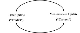
Figure 1: The estimate process of the discrete-time Kalman filter.

The estimate process alluded to above is delineated in Fig. 1. As shown, the Kalman filter performs two operations: time update and measurement update. The time update equations are (9a) and (9b), while the measurement update equations are (9c)–(9e). The time update equations “predict” the state and estimate errors at time $k+1$ from those at time $k$, while the measurement update equations adjust the priori estimate by using the measurement $z_{i}(k)$ according to the Kalman gain $k_{i}(k)$, which is obtained by minimizing $p_{i}(k)$.

Substituting the input (4) into system (3) leads to the closed-loop system

$$\begin{split}&x_{i}^{1}(k+1)\\ =\,&x_{i}^{1}(k)-\epsilon\sum_{j=1}^{N}\theta_{ij}a_{ij}\left(\hat{x}_{i}^{1}(k|k-\tau)-\hat{x}_{j}^{1}(k|k-\tau)\right)\\ &+\alpha\left(\hat{r}_{i}(k|k-\tau)-\hat{x}_{i}^{1}(k|k-\tau)\right)\\ &x_{i}^{2}(k+1)\\ =\,&x_{i}^{2}(k)-\epsilon\sum_{j=1}^{N}\theta_{ij}a_{ij}\left(\hat{x}_{i}^{2}(k|k-\tau)-\hat{x}_{j}^{2}(k|k-\tau)\right)\\ &+\alpha\left(\hat{x}_{i}^{1}(k|k-\tau)-\hat{x}_{i}^{2}(k|k-\tau)\right)\\ &\hskip 86.72267pt\vdots\\ &x_{i}^{n}(k+1)\\ =\,&x_{i}^{n}(k)-\epsilon\sum_{j=1}^{N}\theta_{ij}a_{ij}\left(\hat{x}_{i}^{n}(k|k-\tau)-\hat{x}_{j}^{n}(k|k-\tau)\right)\\ &+\alpha\left(\hat{x}_{i}^{n-1}(k|k-\tau)-\hat{x}_{i}^{n}(k|k-\tau)\right),\end{split}$$ (10)

which can be written in a vector format as

$$\begin{split}\boldsymbol{x}^{1}(k+1)=\,&\boldsymbol{x}^{1}(k)-\epsilon\widetilde{L}\hat{\boldsymbol{x}}^{1}(k|k-\tau)\\ &+\alpha\left(\hat{\boldsymbol{r}}(k|k-\tau)-\hat{\boldsymbol{x}}^{1}(k|k-\tau)\right)\\ \boldsymbol{x}^{2}(k+1)=\,&\boldsymbol{x}^{2}(k)-\epsilon\widetilde{L}\hat{\boldsymbol{x}}^{2}(k|k-\tau)\\ &+\alpha\left(\hat{\boldsymbol{x}}^{1}(k|k-\tau)-\hat{\boldsymbol{x}}^{2}(k|k-\tau)\right)\\ &\vdots\\ \boldsymbol{x}^{n}(k+1)=\,&\boldsymbol{x}^{n}(k)-\epsilon\widetilde{L}\hat{\boldsymbol{x}}^{n}(k|k-\tau)\\ &+\alpha\left(\hat{\boldsymbol{x}}^{n-1}(k|k-\tau)-\hat{\boldsymbol{x}}^{n}(k|k-\tau)\right),\end{split}$$ (11)

where

$$\begin{split}\boldsymbol{x}^{p}(k)=\,&[{x_{1}^{p}(k)},{x_{2}^{p}(k)},\dots,{x_{N}^{p}(k)}]^{\mathrm{T}}\\ \hat{\boldsymbol{x}}^{p}(k|k-\tau)=\,&[{\hat{x}_{1}^{p}(k|k-\tau)},{\hat{x}_{2}^{p}(k|k-\tau)},\dots,{\hat{x}_{N}^{p}(k|k-\tau)}]^{\mathrm{T}}\\ \hat{\boldsymbol{r}}(k|k-\tau)=\,&[{\hat{r}_{1}(k|k-\tau)},{\hat{r}_{2}(k|k-\tau)},\dots,{\hat{r}_{N}(k|k-\tau)}]^{\mathrm{T}}.\end{split}$$

Here, $\widetilde{L}$ is a stochastic Laplacian matrix, changing within the possible set $\{L_{1},L_{2},\dots,L_{s}\}$, where $L_{m}=\left[l_{ij}\right]_{m}$ is the Laplacian matrix associated with $\mathcal{G}_{m}$, i.e.,

$$[\l_{ij}]_{m}=\left\{\begin{array}[]{lr}\sum\limits_{q=1}^{N}[\theta_{iq}]_{m}a_{iq},&i=j,\\ -[\theta_{ij}]_{m}a_{ij},&i\neq j.\end{array}\right.$$

For future use, let

$$\begin{split}[\overline{l}_{ij}]_{m}=\mathbb{E}[[l_{ij}]_{m}]=\left\{\begin{array}[]{lr}\sum\limits_{q=1}^{N}(1-p_{iq})a_{iq},&i=j,\\ -(1-p_{ij})a_{ij},&i\neq j.\end{array}\right.\end{split}$$

The following gives a useful result regarding the expecation of the Laplacian matrix $\tilde{L}$. The result will be employed in the convergence analysis in the next section.

Lemma 1 ([33])

For multi-agent system (10) with a connected communication network, the expected Laplacian matrix, $\overline{L}\triangleq\mathbb{E}[\widetilde{L}]$, has only one zero eigenvalue, i.e.,

$$0=\lambda_{\overline{L},1}<\lambda_{\overline{L},2}\leq\dots\leq\lambda_{\overline{L},N}.$$

The advantages of the multi-stage DAT system (10) are as follows: firstly, it does not involve integral control actions or input derivatives, thus exhibits robustness to initialization errors; secondly, the proposed multi-state scheme enables the possibility of making a trade-off among the communication/computation cost (i.e., the number of stages), the tracking error and the convergence time; thirdly, the proposed scheme takes input delay, packet-drops, and reference noise into consideration, making it more feasible for practical applications.

5 Convergence Analysis

In this section, the convergence of the proposed algorithm embedded in system (10) is analyzed. It is first to show that the Kalman filter (9) is stable.

Lemma 2

If the second part of Assumption 1 holds, then the Kalman filter (9) is stable, i.e.,

$$\lim_{k\to\infty}\mathbb{E}[\hat{r}_{i}(k)-r_{i}(k)]=0.$$ (12)

Proof 5.1.

It follows from (ii) of Assumption 1 that the reference (4) is uniformly observable and uniformly controllable. That is, the matrix pair $[1,\psi_{i}^{-\frac{1}{2}}(k)h_{i}]$ is uniformly observable, and the matrix pair $[1,\phi_{i}^{\frac{1}{2}}(k)]$ is uniformly controllable. The stability result (12) then follows immediately from [32].

In what follows, the performance of the multi-stage DAT system (10) is analyzed. Let

$$\boldsymbol{r}^{*}\triangleq\lim_{k\to\infty}\mathbb{E}[\boldsymbol{r}(k)]=[r_{1}^{*},r_{2}^{*},\dots,r_{N}^{*}]^{\mathrm{T}},~{}\boldsymbol{r}^{*}\in\mathbb{R}^{N},$$

where $r_{i}^{*}\triangleq\lim_{k\to\infty}\mathbb{E}[r_{i}(k)],i={1,\dots,N}$. Note that $\boldsymbol{r}^{*}$ is well defined due to Assumption 1. The following result characterizes agents’ stationary states in terms of $\boldsymbol{r}^{*}$.

Lemma 5.2.

For the multi-agent system (10) with a connected communication network, if Assumption 1 holds, $\epsilon\in(0,\frac{1}{2\overline{d}_{\max}})$, $\alpha\in(0,1-\epsilon\overline{d}_{\max})$, and $k_{x},k_{r}\in(0,1)$, then $\boldsymbol{x}^{p,*}\triangleq\lim_{k\to\infty}\mathbb{E}[\boldsymbol{x}^{p}(k)]$ exists and is given by

$$\boldsymbol{x}^{p,*}=(\alpha\boldsymbol{\mathrm{I}}+\epsilon\overline{L})^{-p}\alpha^{p}\boldsymbol{r}^{*}.$$

Proof 5.3.

Without loss of generality, only the first-stage state is analyzed here. The proof for the other stages is similar and is hence omitted.

Replacing $k-\tau$ with $k$ in (7) yields

$$\begin{split}\hat{x}_{i}^{1}(k+1|k)&=\hat{x}_{i}^{1}(k|k-1)+k_{x}(x_{i}^{1}(k)\\ &\quad-\hat{x}_{i}^{1}(k|k-1))+u_{i}^{1}(k).\end{split}$$ (13)

Let $e_{i}^{1}(k)=x_{i}^{1}(k)-\hat{x}_{i}^{1}(k|k-1)$. Subtracting (13) from (10) leads to

$$e_{i}^{1}(k+1)=e_{i}^{1}(k)-k_{x}e_{i}^{1}(k)=(1-k_{x})e_{i}^{1}(k).$$ (14)

Applying (8) recursively gives

$$\begin{split}&\hat{x}_{i}^{1}(k|k-\tau)\\ =\,&\hat{x}_{i}^{1}(k-1|k-\tau)+u_{i}^{1}(k-1)\\ =\,&\hat{x}_{i}^{1}(k-\tau+1|k-\tau)+\sum_{l=2}^{\tau}u_{i}^{1}(k-\tau+l-1)\\ =\,&\hat{x}_{i}^{1}(k-\tau|k-\tau-1)+\sum_{l=2}^{\tau}u_{i}^{1}(k-\tau+k-1)\\ &+u_{i}^{1}(k-\tau)+k_{x}(x_{i}^{1}(k-\tau)\\ &-\hat{x}_{i}^{1}(k-\tau|k-\tau-1))\\ =\,&\hat{x}_{i}^{1}(k-\tau|k-\tau-1)+\sum_{l=1}^{\tau}u_{i}^{1}(k-\tau+l-1)\\ &+k_{x}(x_{i}^{1}(k-\tau)-\hat{x}_{i}^{1}(k-\tau|k-\tau-1)).\end{split}$$ (15)

Similarly, applying (10) recursively yields

$$\begin{split}x_{i}^{1}(k)=x_{i}^{1}(k-\tau)+\sum_{l=1}^{\tau}u_{i}^{1}(k-\tau+l-1).\end{split}$$ (16)

Subtracting (16) from (15) leads to

$$\begin{split}&\hat{x}_{i}^{1}(k|k-\tau)\\ =\,&x_{i}^{1}(k)+k_{x}(x_{i}^{1}(k-\tau)-\hat{x}_{i}^{1}(k-\tau|k-\tau-1))\\ &+\hat{x}_{i}^{1}(k-\tau|k-\tau-1)-x_{i}^{1}(k-\tau)\\ =\,&x_{i}^{1}(k)+k_{x}e_{i}^{1}(k-\tau)-e_{i}^{1}(k-\tau)\\ =\,&x_{i}^{1}(k)+(k_{x}-1)e_{i}^{1}(k-\tau).\end{split}$$ (17)

It follows from (14) and (17) that

$$\hat{x}_{i}^{1}(k|k-\tau)=x_{i}^{1}(k)-e_{i}^{1}(k-\tau+1).$$ (18)

For the reference signals, define $e^{\prime}_{i}(k)=\hat{r}_{i}(k)-\hat{r}_{i}(k|k-1)$. It then follows that

$$e^{\prime}_{i}(k+1)=e^{\prime}_{i}(k)-k_{r}e^{\prime}_{i}(k)=(1-k_{r})e^{\prime}_{i}(k),$$ (19)

and

$$\hat{r}_{i}(k|k-\tau)=\hat{r}_{i}(k)-e^{\prime}_{i}(k-\tau+1).$$ (20)

Using (18) and (20), it follows from (10) that

$$\begin{split}&x_{i}^{1}(k+1)\\ =\,&x_{i}^{1}(k)-\epsilon\sum_{j=1}^{N}\theta_{ij}a_{ij}\left(x_{i}^{1}(k)-x_{j}^{1}(k)\right)\\ &+\epsilon\sum_{j=1}^{N}\theta_{ij}a_{ij}\left(e_{i}^{1}(k-\tau+1)-e_{j}^{1}(k-\tau+1)\right)\\ &+\alpha\left(\hat{r}_{i}(k)-e^{\prime}_{i}(k-\tau+1)\right)\\ &-\alpha\left(x_{i}^{1}(k)-e_{i}^{1}(k-\tau+1)\right).\end{split}$$ (21)

Since $x_{i}^{1}(k)$ and $e_{i}^{1}(k-\tau+1)$ are independent of $\theta_{ij}$ at time $k$, taking mathematical expectation on both sides of (21) yields

$$\begin{split}&\mathbb{E}[x_{i}^{1}(k+1)]\\ =\,&\mathbb{E}[x_{i}^{1}(k)]-\epsilon\sum_{j=1}^{N}\mathbb{E}[\theta_{ij}]a_{ij}\mathbb{E}\left[x_{i}^{1}(k)-x_{j}^{1}(k)\right]\\ &+\epsilon\sum_{j=1}^{N}\mathbb{E}[\theta_{ij}]a_{ij}\mathbb{E}\left[e_{i}^{1}(k-\tau+1)-e_{j}^{1}(k-\tau+1)\right]\\ &+\alpha\left(\mathbb{E}[\hat{r}_{i}(k)]-\mathbb{E}[e^{\prime}_{i}(k-\tau+1)]\right)\\ &-\alpha\left(\mathbb{E}[x_{i}^{1}(k)]-\mathbb{E}[e_{i}^{1}(k-\tau+1)]\right).\end{split}$$ (22)

It then follows from (2) that $\mathbb{E}[\theta_{ij}]=1-p_{ij}$, which together with (22) leads to

$$\begin{split}&\mathbb{E}[x_{i}^{1}(k+1)]\\ =\,&\mathbb{E}[x_{i}^{1}(k)]-\epsilon\sum_{j=1}^{N}(1-p_{ij})a_{ij}\left(\mathbb{E}[x_{i}^{1}(k)]-\mathbb{E}[x_{j}^{1}(k)]\right)\\ &+\epsilon\sum_{j=1}^{N}(1-p_{ij})a_{ij}\left(\mathbb{E}[e_{i}^{1}(k-\tau+1)]-\mathbb{E}[e_{j}^{1}(k-\tau+1)]\right)\\ &+\alpha\left(\mathbb{E}[\hat{r}_{i}(k)]-\mathbb{E}[e^{\prime}_{i}(k-\tau+1)]\right)\\ &-\alpha\left(\mathbb{E}[x_{i}^{1}(k)]-\mathbb{E}[e_{i}^{1}(k-\tau+1)]\right).\end{split}$$

Let

$$\begin{split}\mathbb{E}[\Delta x_{i}^{1}(k)]&\triangleq\mathbb{E}[x_{i}^{1}(k)]-\mathbb{E}[x_{i}^{1}(k-1)]\\ \mathbb{E}[\Delta e_{i}^{1}(k)]&\triangleq\mathbb{E}[e_{i}^{1}(k)]-\mathbb{E}[e_{i}^{1}(k-1)]\\ \mathbb{E}[\Delta\hat{r}_{i}(k)]&\triangleq\mathbb{E}[\hat{r}_{i}(k)]-\mathbb{E}[\hat{r}_{i}(k-1)]\\ \mathbb{E}[\Delta e^{\prime}_{i}(k)]&\triangleq\mathbb{E}[e^{\prime}_{i}(k)]-\mathbb{E}[e^{\prime}_{i}(k-1)].\\ \end{split}$$

It follows that

$$\begin{split}&\mathbb{E}[\Delta x_{i}^{1}(k+1)]\\ =\,&\mathbb{E}[\Delta x_{i}^{1}(k)]-\epsilon\sum_{j=1}^{N}(1-p_{ij})a_{ij}(\mathbb{E}[\Delta x_{i}^{1}(k)]-\mathbb{E}[\Delta x_{j}^{1}(k)])\\ &-\epsilon\sum_{j=1}^{N}(1-p_{ij})a_{ij}(\Delta\mathbb{E}[e_{j}^{1}(k-\tau+1)]\\ &-\mathbb{E}[\Delta e_{i}^{1}(k-\tau+1)])\\ &+\alpha\mathbb{E}[\Delta\hat{r}_{i}(k)]-\alpha\mathbb{E}[\Delta e^{\prime}_{i}(k-\tau+1)]\\ &-\alpha\mathbb{E}[\Delta x_{i}^{1}(k)]+\alpha\mathbb{E}[\Delta e_{i}^{1}(k-\tau+1)].\end{split}$$ (23)

Define

$$\begin{split}\mathbb{E}[\Delta\boldsymbol{x}^{1}(k)]=[\mathbb{E}[\Delta x_{1}^{1}(k)],\mathbb{E}[\Delta x_{2}^{1}(k)],\dots,\mathbb{E}[\Delta x_{N}^{1}(k)]]^{\mathrm{T}}\\ \mathbb{E}[\Delta{\boldsymbol{e}}^{1}(k-\tau+1)]=[\mathbb{E}[\Delta e_{1}^{1}(k-\tau+1)],\mathbb{E}[\Delta e_{2}^{1}(k-\tau+1)],\\ \qquad\dots,\mathbb{E}[\Delta e_{N}^{1}(k-\tau+1)]]^{\mathrm{T}}\\ \mathbb{E}[\Delta\hat{\boldsymbol{r}}(k)]=[\mathbb{E}[\Delta\hat{r}_{1}(k)],\mathbb{E}[\Delta\hat{r}_{2}(k)],\dots,\mathbb{E}[\Delta\hat{r}_{N}(k)]]^{\mathrm{T}}\\ \mathbb{E}[\Delta\boldsymbol{e^{\prime}}(k-\tau+1)]=[\mathbb{E}[\Delta e^{\prime}_{1}(k-\tau+1)],\mathbb{E}[\Delta e^{\prime}_{2}(k-\tau+1)],\\ \qquad\dots,\mathbb{E}[\Delta e^{\prime}_{N}(k-\tau+1)]]^{\mathrm{T}}.\end{split}$$

Eq. (23) can be written as

$$\begin{split}\mathbb{E}[\Delta\boldsymbol{x}^{1}(k+1)]=&\,[(1-\alpha)\boldsymbol{\mathrm{I}}-\epsilon\overline{L}]\mathbb{E}[\Delta\boldsymbol{x}^{1}(k)]\\ &+(\alpha\boldsymbol{\mathrm{I}}+\epsilon\overline{L})\mathbb{E}[\Delta\boldsymbol{e}^{1}(k-\tau+1)]\\ &+\alpha\mathbb{E}[\Delta\hat{\boldsymbol{r}}(k)]-\alpha\mathbb{E}[\Delta\boldsymbol{e^{\prime}}(k-\tau+1)].\end{split}$$ (24)

Using (14) and (19), Eq. (24) can be rewritten in a compact form as

$$\begin{split}&\left[\begin{array}[]{ccc}\mathbb{E}[\Delta\boldsymbol{x}^{1}(k+1)]\\ \mathbb{E}[\Delta\boldsymbol{e}^{1}(k-\tau+2)]\\ \mathbb{E}[\Delta\boldsymbol{e^{\prime}}(k-\tau+2)]\end{array}\right]\\ =&M\left[\begin{array}[]{ccc}\mathbb{E}[\Delta\boldsymbol{x}^{1}(k)]\\ \mathbb{E}[\Delta\boldsymbol{e}^{1}(k-\tau+1)]\\ \mathbb{E}[\Delta\boldsymbol{e^{\prime}}(k-\tau+1)]\end{array}\right]+\alpha\left[\begin{array}[]{ccc}\mathbb{E}[\Delta\hat{\boldsymbol{r}}(k)]\\ 0\\ 0\end{array}\right],\end{split}$$ (25)

where

$$\begin{split}M\triangleq\left[\begin{array}[]{ccc}(1-\alpha)\boldsymbol{\mathrm{I}}-\epsilon\overline{L}&\alpha\boldsymbol{\mathrm{I}}+\epsilon\overline{L}&-\alpha\\ 0&(1-k_{x})\boldsymbol{\mathrm{I}}&0\\ 0&0&(1-k_{r})\boldsymbol{\mathrm{I}}\end{array}\right].\end{split}$$ (26)

Taking mathematical expectation on both sides of (4) leads to

$$\mathbb{E}[r_{i}(k+1)]=\mathbb{E}[r_{i}(k)]+\mathbb{E}[v_{i}(k)].$$

Based on Assumption 1 and (12), one has

$$\lim_{k\to\infty}\mathbb{E}[\hat{r}_{i}(k)]\to r_{i}^{*}(k),$$ (27)

which further leads to $\lim_{k\to\infty}\mathbb{E}[\Delta\hat{\boldsymbol{r}}(k)]\to 0$.

Due to (27), as $k\to\infty$, Eq. (25) becomes

$$\begin{split}&\left[\begin{array}[]{ccc}\mathbb{E}[\Delta\boldsymbol{x}^{1}(k+1)]\\ \mathbb{E}[\Delta\boldsymbol{e}^{1}(k-\tau+2)]\\ \mathbb{E}[\Delta\boldsymbol{e^{\prime}}(k-\tau+2)]\end{array}\right]=M\left[\begin{array}[]{ccc}\mathbb{E}[\Delta\boldsymbol{x}^{1}(k)]\\ \mathbb{E}[\Delta\boldsymbol{e}^{1}(k-\tau+1)]\\ \mathbb{E}[\Delta\boldsymbol{e^{\prime}}(k-\tau+1)]\end{array}\right].\end{split}$$ (28)

It follows that the system (28) is asymptotically stable if and only if all the eigenvalues of the matrix $M$ lie within the unit circle. Furthermore, (26) suggests that the eigenvalues of the matrix $M$ coincide with the eigenvalues of the matrices $(1-\alpha)\boldsymbol{\mathrm{I}}-\epsilon\overline{L}$, $(1-k_{x})\boldsymbol{\mathrm{I}}$ and $(1-k_{r})\boldsymbol{\mathrm{I}}$.

For the matrices $(1-k_{x})\boldsymbol{\mathrm{I}}$ and $(1-k_{r})\boldsymbol{\mathrm{I}}$, by choosing $k_{x},k_{r}\in(0,1)$, all the eigenvalues of the two matrices are within the unit circle. For the matrix $(1-\alpha)\boldsymbol{\mathrm{I}}-\epsilon\overline{L}$, it follows from (3) that $\overline{L}=\sum_{m=1}^{s}\mathbb{P}(\widetilde{\mathcal{G}}=\mathcal{G}_{m})L_{m}$. Denote the $i$th eigenvalue of $\overline{L}$ by $\lambda_{\overline{L},i}$. According to the Gerschgorin disc theorem, the expected Laplacian matrix has all its eigenvalues located within $[0,2\overline{d}_{\max}]$, where $\overline{d}_{\max}$ is the maximum degree of the expected graph $\overline{\mathcal{G}}$. It thus follows that

$$0=\lambda_{\overline{L},1}<\lambda_{\overline{L},2}\leq\dots\leq\lambda_{\overline{L},N}\leq 2\overline{d}_{\max}.$$

Since $\overline{L}$ is a symmetric matrix, the matrix $(1-\alpha)\boldsymbol{\mathrm{I}}_{N}-\epsilon\overline{L}$ is symmetric. Consequently, all the eigenvalues are real and are given by

$$\lambda_{i}=1-\alpha-\epsilon\lambda_{\overline{L},i}.$$ (29)

Since $\alpha\in(0,1-\epsilon\overline{d}_{\max})$ and $\epsilon\in(0,\frac{1}{2\overline{d}_{\max}})$, it follows that the eigenvalues of (29) satisfy $\lambda_{i}\in(0,1),~{}i\in\{1,\dots,N\}$. As all eigenvalues of $M$ are within the unit circle, the dynamical system (28) is asymptotically stable.

Let $\boldsymbol{x}^{1,*}$ denote the expected steady state. That is,

$$\boldsymbol{x}^{1,*}\triangleq\lim_{k\to\infty}\mathbb{E}[\boldsymbol{x}^{1}(k)]=[x_{1}^{1,*},x_{2}^{1,*},\dots,x_{N}^{1,*}]^{T},$$

where $x_{i}^{1,*}\triangleq\lim_{K\to\infty}\mathbb{E}[x_{i}^{1}(k)],i=1,2,\dots,N$, represents the expected steady state at stage $1$ of agent $i$. As the asymptotic convergence of (28) is ensured, $\boldsymbol{x}^{1,*}$ is well defined. The system (28) is asymptotically stable, i.e., $\mathbb{E}[\Delta\boldsymbol{e}^{1}(k-\tau+2)]\to 0$, $\mathbb{E}[\Delta\boldsymbol{e^{\prime}}(k-\tau+2)]\to 0$, $\mathbb{E}[\Delta\boldsymbol{x}^{1}(k)]\to 0$ as $k\to\infty$. As a result,

$$\lim_{k\to\infty}\mathbb{E}[\boldsymbol{x}^{1}(k+1)]\to\mathbb{E}[\boldsymbol{x}^{1}(k)]\to\boldsymbol{x}^{1,*}.$$ (30)

It follows from (17) and (19) that $\mathbb{E}[e_{i}^{1}(k)]\to 0$ and $\mathbb{E}[e^{\prime}_{i}(k)]\to 0$ as $k\to\infty$, which further leads (18) and (20) to

$$\begin{split}\mathbb{E}[\hat{x}_{i}^{1}(k|k-\tau)]&\to\mathbb{E}[x_{i}^{1}(k)]\\ \mathbb{E}[\hat{r}_{i}(k|k-\tau)]&\to\mathbb{E}[\hat{r}_{i}(k)],~{}\text{as $k\to\infty$}.\end{split}$$ (31)

Eq. (11) gives

$$\begin{split}\mathbb{E}[\boldsymbol{x}^{1}(k+1)]=&\mathbb{E}[\boldsymbol{x}^{1}(k)]-\epsilon\overline{L}\mathbb{E}[\hat{\boldsymbol{x}}^{1}(k|k-\tau)]\\ &+\alpha\left(\mathbb{E}[\hat{\boldsymbol{r}}(k)]-\mathbb{E}[\hat{\boldsymbol{x}}^{1}(k|k-\tau)]\right).\end{split}$$ (32)

Using (27), (30) and (31), it follows from (32) that

$$\begin{split}\boldsymbol{x}^{1,*}=\boldsymbol{x}^{1,*}-\epsilon\overline{L}\boldsymbol{x}^{1,*}+\alpha\left(\boldsymbol{r}^{*}-\boldsymbol{x}^{1,*}\right).\end{split}$$

The expected steady-state equilibrium at the first stage is then given by

$$\boldsymbol{x}^{1,*}=(\alpha\boldsymbol{\mathrm{I}}+\epsilon\overline{L})^{-1}\alpha\boldsymbol{r}^{*}.$$ (33)

For the remaining $n-1$ stages, it can be shown similarly that

$$\boldsymbol{x}^{p,*}=(\alpha\boldsymbol{\mathrm{I}}+\epsilon\overline{L})^{-1}\alpha\boldsymbol{x}^{p-1,*},$$ (34)

where $\boldsymbol{x}^{p,*}\triangleq[x_{1}^{p,*},x_{2}^{p,*},\dots,x_{N}^{p,*}]^{\mathrm{T}}\in\mathbb{R}^{N},p=1,2,\dots,n$, represents the expected steady state at stage $p$ and $x_{i}^{p,*}\triangleq\lim_{k\to\infty}\mathbb{E}[x_{i}^{p}(k)],i=1,2,\dots,N$. Combining (33) and (34) gives

$$\boldsymbol{x}^{p,*}=(\alpha\boldsymbol{\mathrm{I}}+\epsilon\overline{L})^{-p}\alpha^{p}\boldsymbol{r}^{*}.$$

The proof is thus completed.

The main result of this section is the following theorem.

Theorem 5.4.

For the system (10) with a connected communication network, if Assumption 1 holds, $\epsilon\in(0,\frac{1}{2\overline{d}_{\max}})$, $\alpha\in(0,1-\epsilon\overline{d}_{\max})$, and $k_{x},k_{r}\in(0,1)$, then

$$\limsup_{k\to\infty}\left\|\bar{r}^{*}\boldsymbol{1}_{N}-\boldsymbol{x}^{n,*}\right\|_{2}\leq\left(\frac{\alpha}{\alpha+\epsilon\lambda_{\overline{L},2}}\right)^{n}\|\widetilde{\boldsymbol{r}}^{*}\|_{2},$$

where $\widetilde{\boldsymbol{r}}^{*}\triangleq(\boldsymbol{r}^{*}-\bar{r}^{*}\boldsymbol{1}_{N})$ and $\bar{r}^{*}\triangleq\frac{1}{N}\sum_{i=1}^{N}r_{i}^{*}$.

Proof 5.5.

It follows from Lemma 5.2 that

$$\boldsymbol{x}^{p,*}=(\alpha\boldsymbol{\mathrm{I}}+\epsilon\overline{L})^{-p}\alpha^{p}\boldsymbol{r}^{*}.$$

The eigenvalues of the matrix $(\alpha\boldsymbol{\mathrm{I}}+\epsilon\overline{L})^{-p}$ are given by

$$\lambda_{i}^{\prime}=\left(\frac{1}{\alpha+\epsilon\lambda_{\overline{L},i}}\right)^{p},$$

where $\lambda_{\overline{L},i}$ denotes the $i$th eigenvalue of the matrix $\overline{L}$, and $\boldsymbol{v}_{i}$ is the corresponding eigenvector. The columns of the matrix $V=[\boldsymbol{v}_{1},\boldsymbol{v}_{2},\dots,\boldsymbol{v}_{N}]$ are orthonormal. Consequently, $\overline{L}$ can be expressed as $\overline{L}=V\Lambda_{\overline{L}}V^{T}=\sum_{i=1}^{N}\lambda_{\overline{L},i}\boldsymbol{v}_{i}\boldsymbol{v}_{i}^{T}$, where $\Lambda_{\overline{L}}=\text{diag}\{\lambda_{\overline{L},1},\lambda_{\overline{L},2},\dots,\lambda_{\overline{L},N}\}$ and $\boldsymbol{v}_{1}=\frac{1}{\sqrt{N}}\boldsymbol{1}_{N}$. Hence,

$$\begin{split}\boldsymbol{x}^{p,*}=&(\alpha\boldsymbol{\mathrm{I}}+\epsilon\overline{L})^{-p}\alpha^{p}\boldsymbol{r}^{*}\\ =&(\alpha V\boldsymbol{\mathrm{I}}V^{T}+\epsilon V\Lambda_{\overline{L}}V^{T})^{-p}\alpha^{p}\boldsymbol{r}^{*}\\ =&(V(\alpha\boldsymbol{\mathrm{I}}+\epsilon\Lambda_{\overline{L}})V^{T})^{-p}\alpha^{p}\boldsymbol{r}^{*}\\ =&\sum_{i=1}^{N}\left(\frac{1}{\alpha+\epsilon\lambda_{\overline{L},i}}\right)^{p}\boldsymbol{v}_{i}\boldsymbol{v}_{i}^{T}\alpha^{p}\boldsymbol{r}^{*}\\ =&\sum_{i=1}^{N}\left(\frac{\alpha}{\alpha+\epsilon\lambda_{\overline{L},i}}\right)^{p}\boldsymbol{v}_{i}\boldsymbol{v}_{i}^{T}\boldsymbol{r}^{*}\\ =&\sum_{i=2}^{N}\left(\frac{\alpha}{\alpha+\epsilon\lambda_{\overline{L},i}}\right)^{p}\boldsymbol{v}_{i}\boldsymbol{v}_{i}^{T}\boldsymbol{r}^{*}+\boldsymbol{v}_{1}\boldsymbol{v}_{1}^{T}\boldsymbol{r}^{*}\\ =&\sum_{i=2}^{N}\left(\frac{\alpha}{\alpha+\epsilon\lambda_{\overline{L},i}}\right)^{p}\boldsymbol{v}_{i}\boldsymbol{v}_{i}^{T}\boldsymbol{r}^{*}+\frac{1}{N}\boldsymbol{1}_{N\times N}\boldsymbol{r}^{*}\\ =&\sum_{i=2}^{N}\left(\frac{\alpha}{\alpha+\epsilon\lambda_{\overline{L},i}}\right)^{p}\boldsymbol{v}_{i}\boldsymbol{v}_{i}^{T}\boldsymbol{r}^{*}+\bar{r}^{*}\boldsymbol{1}_{N}.\end{split}$$ (35)

It follows from (35) that

$$\begin{split}&\quad\limsup_{k\to\infty}\|\bar{r}^{*}\boldsymbol{1}_{N}-\boldsymbol{x}^{n,*}\|_{2}\\ &=\left\|\sum_{i=2}^{N}\left(\frac{\alpha}{\alpha+\epsilon\lambda_{\overline{L},i}}\right)^{n}\boldsymbol{v}_{i}\boldsymbol{v}_{i}^{T}\boldsymbol{r}^{*}\right\|_{2}\\ &\leq\left(\frac{\alpha}{\alpha+\epsilon\lambda_{\overline{L},2}}\right)^{n}\left\|\sum_{i=2}^{N}\boldsymbol{v}_{i}\boldsymbol{v}_{i}^{T}\boldsymbol{r}^{*}\right\|_{2}\\ &\leq\left(\frac{\alpha}{\alpha+\epsilon\lambda_{\overline{L},2}}\right)^{n}\left\|\sum_{i=1}^{N}\boldsymbol{v}_{i}\boldsymbol{v}_{i}^{T}\boldsymbol{r}^{*}-\boldsymbol{v}_{1}\boldsymbol{v}_{1}^{T}\boldsymbol{r}^{*}\right\|_{2}\\ &\leq\left(\frac{\alpha}{\beta}\right)^{n}\|\widetilde{\boldsymbol{r}}^{*}\|_{2},\end{split}$$

where $\widetilde{\boldsymbol{r}}^{*}:=(\boldsymbol{r}^{*}-\bar{r}^{*}\boldsymbol{1}_{N})$.

On the one hand, Theorem 5.4 shows the possibility of achieving mean-squared DAT in the presence of input delay, reference noise, and packet-drops. As the stage number $n$ goes to infinity, the tracking error will approach zero, i.e, the control objective (5) will be achieved. On the other hand, a larger stage number $n$ will induce a higher communication/computation cost for the agents, indicating that there exists trade-off between the tracking error and communication/computation cost.

6 Simulation

In this section, a numerical example is presented to verify Theorem 5.4.

A system consisting of $N=4$ nodes is considered. The communication network topology is given in Fig. 2.

Figure 2: The communication network topology

Assume that the packet-drop probability $p_{ij}=0.5$, $\forall\,(i,j)\in\mathcal{E}$. The actual network topology can vary from one of the eight network topologies shown in Fig. 3 due to packet-drops.

(a) $\mathcal{G}_{1}$

(b) $\mathcal{G}_{2}$

(c) $\mathcal{G}_{3}$

(d) $\mathcal{G}_{4}$

(e) $\mathcal{G}_{5}$

(f) $\mathcal{G}_{6}$

(g) $\mathcal{G}_{7}$

(h) $\mathcal{G}_{8}$

Figure 3: The possible actual network topologies

Their corresponding Laplacian matrices are given respectively by

$$L_{1} =\left[\begin{array}[]{cccc}1&-1&0&0\\ -1&2&-1&0\\ 0&-1&2&-1\\ 0&0&-1&1\end{array}\right], L_{2} =\left[\begin{array}[]{cccc}0&0&0&0\\ 0&0&0&0\\ 0&0&0&0\\ 0&0&0&0\end{array}\right]$$ (44)

$$L_{3} =\left[\begin{array}[]{cccc}0&0&0&0\\ 0&1&-1&0\\ 0&-1&2&-1\\ 0&0&-1&1\end{array}\right], L_{4} =\left[\begin{array}[]{cccc}0&0&0&0\\ 0&0&0&0\\ 0&0&1&-1\\ 0&0&-1&1\end{array}\right]$$ (53)

$$L_{5} =\left[\begin{array}[]{cccc}1&-1&0&0\\ -1&1&0&0\\ 0&0&1&-1\\ 0&0&-1&1\end{array}\right], L_{6} =\left[\begin{array}[]{cccc}1&-1&0&0\\ -1&1&0&0\\ 0&0&0&0\\ 0&0&0&0\end{array}\right]$$ (62)

$$L_{7} =\left[\begin{array}[]{cccc}1&-1&0&0\\ -1&2&-1&0\\ 0&-1&1&0\\ 0&0&0&0\end{array}\right], L_{8} =\left[\begin{array}[]{cccc}0&0&0&0\\ 0&1&-1&0\\ 0&-1&1&0\\ 0&0&0&0\end{array}\right].$$ (71)

The expected Laplacian matrix $\overline{L}$ is given by

$$\overline{L}=\mathbb{P}(\widetilde{\mathcal{G}}=\mathcal{G}_{1})L_{1}+\mathbb{P}(\widetilde{\mathcal{G}}=\mathcal{G}_{2})L_{2}+\dots+\mathbb{P}(\widetilde{\mathcal{G}}=\mathcal{G}_{8})L_{8}.$$

Fig. 4 shows the expected network topology $\overline{\mathcal{G}}$, the network topology corresponding to $\overline{L}$.

Figure 4: The expected network topology

The reference signals are governed by (4), with $\phi_{i}=0.01$ and $\psi_{i}=1$. Finally, the parameters are chosen as $\epsilon=\frac{1}{8}$, $\alpha=\frac{1}{2}$, and $k_{x}=k_{r}=\frac{1}{2}$. The input delay is set to $\tau=5$.

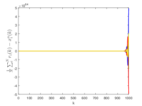
(a) n=10.

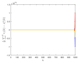
(b) n=100.

Figure 5: Tracking error of the $n$th stage of $x_{i}(k)$ under the DAT algorithm (4).

Fig. 5 shows the tracking error $\frac{1}{N}\sum_{i=1}^{N}r_{i}(k)-x_{i}^{n}(k)$ under the proposed algorithm embedded in system (10) without employing the Kalman filter and state predictor to handle the input delays, packet-drops, and noisy reference signals. It can be observed that the system cannot track the average of the reference signals; instead, the tracking error diverges eventually.

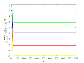
(a) n=10.

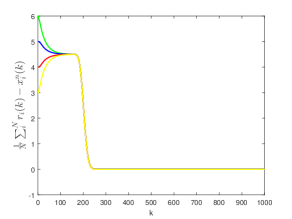
(b) n=100.

Figure 6: Tracking error of the $n$th stage of $x_{i}(k)$ under the DAT algorithm (4).

Fig. 6 shows the tracking error of the proposed DAT algorithm with the Kalman filter and state predictor for different stage number $n$. It can be seen that in both cases the tracking error will finally reach a steady value. Furthermore, as the stage number gets larger, the tracking error gets smaller, which is consistent with Theorem 5.4.

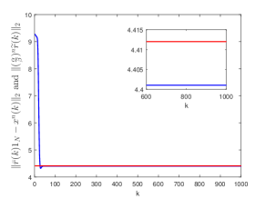
(a) n=10.

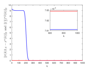
(b) n=100.

Figure 7: The trajectories of $\|\bar{r}(k)\boldsymbol{1}_{N}-\boldsymbol{x}^{n}(k)\|_{2}$ and $\delta=\left(\frac{\alpha}{\beta}\right)^{n}\|\widetilde{\boldsymbol{r}}(k)\|_{2}$.

Fig. 7 shows respectively the trajectories of $\|\bar{r}(k)\boldsymbol{1}_{N}-\boldsymbol{x}^{n}(k)\|_{2}$ and $\delta=\left(\frac{\alpha}{\beta}\right)^{n}\|\widetilde{\boldsymbol{r}}(k)\|_{2}$. The red line corresponds to the trajectory of $\left(\frac{\alpha}{\beta}\right)^{n}\|\widetilde{\boldsymbol{r}}(k)\|_{2}$, while the blue line to the trajectory of $\|\bar{r}(k)\boldsymbol{1}_{N}-\boldsymbol{x}^{n}(k)\|_{2}$. It can be seen that as $k\to\infty$, the inequality $\limsup\|\bar{r}(k)\boldsymbol{1}_{N}-\boldsymbol{x}^{n}(k)\|_{2}\leq\left(\frac{\alpha}{\beta}\right)^{n}\|\widetilde{\boldsymbol{r}}(k)\|_{2}$ holds eventually.

7 Conclusion

This paper demonstrates that DAT algorithms can be seriously hampered by reference noise, packet-drops, and input delays; however, it is still possible to achieve practical DAT by employing appropriate control techniques, such as Kalman filtering and predictive control, to deal with those negative effects.

In summary, the following statements are drawn from this work.

• An explicit expression of the expected stationary states of the agents is obtained and given in terms of the expected values of the references, which also depends on the control gains as well as the number of processing stages.

• The mean-squared tracking error is ultimately upper bounded by the average difference among the reference signals, and as the number of stages goes to infinity, the tracking error will varnish, achieving practical DAT in the sense of mean square.

These results shed new lights on the studies of distributed average tracking and cooperative control of multi-agent systems.

References

- [1] C. Chen and F. Chen, “Discrete-time distributed average tracking for noisy reference signals,” in 2019 Chinese Control Conference (CCC). IEEE, 2019, pp. 5405–5410.
- [2] D. P. Spanos, R. Olfati-Saber, and R. M. Murray, “Distributed sensor fusion using dynamic consensus,” in Proceedings of the 16th IFAC World Congress, 2005, paper code. We-E04-TP/3.
- [3] R. Olfati-Saber and J. S. Shamma, “Consensus filters for sensor networks and distributed sensor fusion,” in Proceedings of the 44th IEEE Conference on Decision and Control (CDC), 2005, pp. 6698–6703.
- [4] H. Bai, R. A. Freeman, and K. M. Lynch, “Distributed kalman filtering using the internal model average consensus estimator,” in Proceedings of the American Control Conference (ACC), 2011, pp. 1500–1505.
- [5] S. Rahili and W. Ren, “Distributed continuous-time convex optimization with time-varying cost functions,” IEEE Transactions on Automatic Control, vol. 62, no. 4, pp. 1590–1605, 2017.
- [6] P. Yang, R. A. Freeman, and K. M. Lynch, “Multi-agent coordination by decentralized estimation and control,” IEEE Transactions on Automatic Control, vol. 53, no. 11, pp. 2480–2496, 2008.
- [7] Y. Sun and M. Lemmon, “Swarming under perfect consensus using integral action,” in Proceedings of the American Control Conference(ACC), 2007, pp. 4594–4599.
- [8] F. Chen and W. Ren, “A connection between dynamic region-following formation control and distributed average tracking,” IEEE transactions on cybernetics, vol. 48, no. 6, pp. 1760–1772, 2017.
- [9] F. Chen and J. Chen, “Minimum-energy distributed consensus control of multi-agent systems: A network approximation approach,” IEEE Transactions on Automatic Control, to be published. [Online]. Available: https://doi.org/10.1109/TAC.2019.2917279
- [10] J. Mei, W. Ren, and J. Chen, “Distributed consensus of second-order multi-agent systems with heterogeneous unknown inertias and control gains under a directed graph,” IEEE Transactions on Automatic Control, vol. 61, no. 8, pp. 2019–2034, 2015.
- [11] D. P. Spanos, R. Olfati-Saber, and R. M. Murray, “Dynamic consensus on mobile networks,” in Proceedings of the 16th IFAC world congress, 2005, paper code. We-A18-TO/1.
- [12] R. A. Freeman, P. Yang, and K. M. Lynch, “Stability and convergence properties of dynamic average consensus estimators,” in Proceedings of the 45th IEEE Conference on Decision and Control (CDC), 2006, pp. 338–343.
- [13] H. Bai, R. A. Freeman, and K. M. Lynch, “Robust dynamic average consensus of time-varying inputs,” in Proceedings of the 49th IEEE Conference on Decision and Control (CDC), 2010, pp. 3104–3109.
- [14] H. Bai, “A two-time-scale dynamic average consensus estimator,” in Proceedings of the 55th IEEE Conference on Decision and Control (CDC), 2016, pp. 75–80.
- [15] F. Chen, Y. Cao, and W. Ren, “Distributed average tracking of multiple time-varying reference signals with bounded derivatives,” IEEE Transactions on Automatic Control, vol. 57, no. 12, pp. 3169–3174, 2012.
- [16] S. Ghapani, W. Ren, F. Chen, and Y. Song, “Distributed average tracking for double-integrator multi-agent systems with reduced requirement on velocity measurements,” Automatica, vol. 81, pp. 1–7, 2017.
- [17] F. Chen, W. Ren, W. Lan, and G. Chen, “Distributed average tracking for reference signals with bounded accelerations,” IEEE Transactions on Automatic Control, vol. 60, no. 3, pp. 863–869, 2015.
- [18] Y. Zhao, Y. Liu, Z. Li, and Z. Duan, “Distributed average tracking for multiple signals generated by linear dynamical systems: An edge-based framework,” Automatica, vol. 75, pp. 158–166, 2017.
- [19] F. Chen, G. Feng, L. Liu, and W. Ren, “Distributed average tracking of networked euler-lagrange systems,” IEEE Transactions on Automatic Control, vol. 60, no. 2, pp. 547–552, 2014.
- [20] Y. Zhao, Y. Liu, G. Wen, X. Yu, and G. Chen, “Distributed average tracking for lipschitz-type of nonlinear dynamical systems,” IEEE transactions on cybernetics, vol. 49, no. 12, pp. 4140–4152, 2018.
- [21] B. Van Scoy, R. A. Freeman, and K. M. Lynch, “Optimal worst-case dynamic average consensus,” in Proceedings of the American Control Conference (ACC), 2015, pp. 5324–5329.
- [22] F. R. A. Van Scoy, Bryan and K. M. Lynch, “Exploiting memory in dynamic average consensus,” in Proceedings of the 53rd Annual Allerton Conference on Communication, Control, and Computing (Allerton), 2015, pp. 258–265.
- [23] Y. Yuan, J. Liu, R. M. Murray, and J. Gonçalves, “Decentralised minimal-time dynamic consensus,” in Proceedings of the American control conference (ACC), 2012, pp. 800–805.
- [24] S. S. Kia, J. Cortés, and S. Martinez, “Dynamic average consensus under limited control authority and privacy requirements,” International Journal of Robust and Nonlinear Control, vol. 25, no. 13, pp. 1941–1966, 2015.
- [25] C. Li, H. Xin, J. Wang, M. Yu, and X. Gao, “Dynamic average consensus with topology balancing under a directed graph,” International Journal of Robust and Nonlinear Control, vol. 29, no. 10, pp. 3014–3026, 2019.
- [26] S. Li and Y. Guo, “Dynamic consensus estimation of weighted average on directed graphs,” International Journal of Systems Science, vol. 46, no. 10, pp. 1839–1853, 2015.
- [27] E. Montijano, J. I. Montijano, C. Sagüés, and S. Martínez, “Robust discrete time dynamic average consensus,” Automatica, vol. 50, no. 12, pp. 3131–3138, 2014.
- [28] M. Franceschelli and A. Gasparri, “Multi-stage discrete time and randomized dynamic average consensus,” Automatica, vol. 99, pp. 69–81, 2019.
- [29] S. S. Kia, B. Van Scoy, J. Cortes, R. A. Freeman, K. M. Lynch, and S. Martinez, “Tutorial on dynamic average consensus: The problem, its applications, and the algorithms,” IEEE Control Systems Magazine, vol. 39, no. 3, pp. 40–72, 2019.
- [30] H. Moradian and S. S. Kia, “On robustness analysis of a dynamic average consensus algorithm to communication delay,” IEEE Transactions on Control of Network Systems, vol. 6, no. 2, pp. 633–641, 2018.
- [31] S.-I. Niculescu, “On delay robustness analysis of a simple control algorithm in high-speed networks,” Automatica, vol. 38, no. 5, pp. 885–889, 2002.
- [32] T. Karvonen, “Stability of linear and non-linear kalman filters,” Master’s thesis, University of Helsinki, 2014.
- [33] W.-M. Zhou and J.-W. Xiao, “Dynamic average consensus and consensusability of general linear multiagent systems with random packet dropout,” Abstract and Applied Analysis, vol. 2013, 2013, article no. 412189.