Optimal estimation of sparse topic models

Abstract

Topic models have become popular tools for dimension reduction and exploratory analysis of text data which consists in observed frequencies of a vocabulary of $p$ words in $n$ documents, stored in a $p\times n$ matrix. The main premise is that the mean of this data matrix can be factorized into a product of two non-negative matrices: a $p\times K$ word-topic matrix $A$ and a $K\times n$ topic-document matrix $W$.

This paper studies the estimation of $A$ that is possibly element-wise sparse, and the number of topics $K$ is unknown. In this under-explored context, we derive a new minimax lower bound for the estimation of such $A$ and propose a new computationally efficient algorithm for its recovery. We derive a finite sample upper bound for our estimator, and show that it matches the minimax lower bound in many scenarios. Our estimate adapts to the unknown sparsity of $A$ and our analysis is valid for any finite $n$, $p$, $K$ and document lengths.

Empirical results on both synthetic data and semi-synthetic data show that our proposed estimator is a strong competitor of the existing state-of-the-art algorithms for both non-sparse $A$ and sparse $A$, and has superior performance is many scenarios of interest.

Keywords: Topic models, minimax estimation, sparse estimation, adaptive estimation, high dimensional estimation, non-negative matrix factorization, separability, anchor words.

1 Introduction

Topic modeling has been a popular and powerful statistical model during the last two decades in machine learning and natural language processing for discovering thematic structures from a corpus of documents. Topic models have wide applications beyond the context in which was originally introduced, to genetics, neuroscience and social science (Blei, 2012), to name just a few areas in which they have been successfully employed.

In the computer science and machine learning literature, topic models were first introduced as latent semantic indexing models by Deerwester et al. (1990); Papadimitriou et al. (1998); Hofmann (1999); Papadimitriou et al. (2000). For uniformity and clarity, we explain our methodology in the language typically associated with this set-up. A corpus of $n$ documents is assumed to follow generative models based on the bag-of-word representation. Specifically, each document $X_{i}\in\mathbb{R}^{p}$ is a vector containing empirical (observed) frequencies of $p$ words from a pre-specified dictionary, generated as

$$X_{i}\sim{1\over N_{i}}\text{Multinomial}_{p}\left(N_{i},\Pi_{i}\right),\quad\text{ for each }i\in[n]:=\{1,2,\ldots,n\}.$$ (1)

Here $N_{i}$ denotes the length (or the number of sampled words) in the $i$th document. The expected frequency vector $\Pi_{i}\in\mathbb{R}^{p}$ is called the word-document vector, and is a convex combination of $K$ word-topic vectors with weights corresponding to the allocation of $K$ topics. Mathematically, one postulates that

$$\Pi_{i}=\sum_{k=1}^{K}A_{\cdot k}W_{ki}$$ (2)

where $A_{\cdot k}=(A_{1k},\ldots,A_{pk})$ is the word-topic vector for the $k$th topic and $W_{\cdot i}=(W_{1i},\ldots,W_{Ki})$ is the allocation of $K$ topics in this $i$th document. From a probabilistic point of view, equation (2) has the conditional probability interpretation

$$\underbrace{\mathbb{P}(\text{word }j\ |\text{ document }i)}_{\Pi_{ji}}=\sum_{k=1}^{K}\underbrace{\mathbb{P}(\text{word }j\ |\text{ topic }k)}_{A_{jk}}\cdot\underbrace{\mathbb{P}(\text{topic }k\ |\text{ document }i)}_{W_{ki}}$$ (3)

for each $j\in[p]$, justified by Bayes’ theorem. As a result, the (expected) word-document frequency matrix $\Pi=(\Pi_{1},\ldots,\Pi_{n})\in\mathbb{R}^{p\times n}$ has the following decomposition

$$\Pi=AW=A(W_{1},\ldots,W_{n}).$$ (4)

The entries of the columns of $\Pi,A$ and $W$ are probabilities, so they are non-negative and sum to one:

$$\sum_{j=1}^{p}\Pi_{ji}=1,\quad\sum_{j=1}^{p}A_{jk}=1,\quad\sum_{k=1}^{K}W_{ki}=1,\quad\text{for any $k\in[K]$ and $i\in[n]$.}$$ (5)

Since the number of topics, $K$, is typically much smaller than $p$ and $n$, the matrix $\Pi$ exhibits a low-rank structure. In the topic modeling literature, the main interest is to recover the matrix $A$ when only the $p\times n$ frequency matrix $X=(X_{1},\ldots,X_{n})$ and the document lengths $N_{1},\ldots,N_{n}$ are observed.

One direction of a large body of work is of Bayesian nature, and the most commonly used prior distribution on $W$ is the Dirichlet distribution (Blei et al., 2003). Posterior inference on $A$ is then typically conducted via variational inference (Blei et al., 2003), or sampling techniques involving MCMC-type solvers (Griffiths and Steyvers, 2004). We refer to Blei (2012) for a in-depth review.

The computational intensive nature of Bayesian approaches, in high dimensions, motivated a separate line of recent work that develops efficient algorithms, with theoretical guarantees, from a frequentist perspective. Anandkumar et al. (2012) proposes an estimation method, with provable guarantees, that employs the third moments of $\Pi$ via a tensor-decomposition. However, the success of this approach requires the topics not be correlated, and in many situations there is strong evidence suggesting the contrary (Blei and Lafferty, 2007; Li and McCallum, 2006).

This motivated another line of work, similar in spirit with the work presented in this paper, which relies on the following separability condition on $A$, and allows for correlated topics.

Assumption 1 (separability)

For each topic $k\in[K]$, there exists at least one word $j$ such that $A_{jk}>0$ and $A_{j\ell}=0$ for any $\ell\neq k$.

The separability condition was first introduced by Donoho and Stodden (2004) to ensure uniqueness in the Non-negative Matrix Factorization (NMF) framework. Arora et al. (2012) introduce the separability condition to the topic model literature with the interpretation that, for each topic, there exist some words which only occur in this topic. These special words are called anchor words (Arora et al., 2012) and guarantee recovery of $A$, coupled with the following condition on $W$ (Arora et al., 2012).

Assumption 2

Assume the matrix $n^{-1}WW^{\top}$ is strictly positive definite.

Finding anchor words is the first step towards the recovery of the desired target $A$. Many algorithms are developed for this purpose, see, for instance, Arora et al. (2012); Bittorf et al. (2012); Arora et al. (2013); Ding et al. (2013); Ke and Wang (2017). All these works require the number of topics $K$ be known, yet in practice $K$ is rarely known. This motivated us Bing et al. (2018) to develop a method that estimates $K$ consistently from the data under the incoherence Condition 3 on the topic-document matrix $W$ given in Section 5. We defer to this for further discussion of other existing methods for finding anchor words.

Despite the wide-spread interest and usage of topic models, most of the existing works are mainly devoted to the computational aspects of estimation, and relatively few works provide statistical guarantees for estimators of $A$. An exception is Arora et al. (2012, 2013) that provide upper bounds for the $\ell_{1}$-loss $\|\widehat{A}-A\|_{1}=\sum_{j=1}^{p}\sum_{k=1}^{K}|\widehat{A}_{jk}-A_{jk}|$ of their estimator. Their analysis allows $K$, $p$ and $N_{i}$ to grow with $n$. Unfortunately, the convergence rate of their estimator is not optimal (Ke and Wang, 2017; Bing et al., 2018). The recent work of Ke and Wang (2017) is the first to establish the minimax lower bound for the estimator of $A$ in topic models for known, fixed $K$. Their estimator provably achieves the minimax optimal rate under appropriate conditions. When $K$ is allowed to grow with $n$, the minimax optimal rate of $\|\widehat{A}-A\|_{1}$ is established in Bing et al. (2018) and an optimal estimation procedure is proposed.

Despite these recent advances, all the aforementioned results are established for a fully dense matrix $A$. In the modern big data era, the dictionary size $p$, the number of documents $n$ and the number of topics $K$ are large, as evidenced by real data in Section 6. Sparsity is likely to happen for large dictionaries ($p$) and when the number of topics $K$ is large, one should expect that there are many words not occurring in all topics, that is, $A_{jk}=\mathbb{P}(\text{word }j\ |\text{ topic }k)=0$ for some $k$.

To the best of our knowledge, the minimax lower bound of $\|\widehat{A}-A\|_{1}$ in the topic model is unknown when the word-topic matrix $A$ is element-wise sparse and no estimation procedure exists tailored to this scenario of sparse $A$ and unknown $K$.

1.1 Our contributions

We summarize our contributions in this paper.

New minimax lower bound for $\|\widehat{A}-A\|_{1}$, when $A$ is sparse.

To understand the difference of estimating a dense $A$ and a entry-wise sparse $A$ in topic models, we first establish the minimax lower bound of estimators of $A$ in Theorem 1 of Section 2. It shows that

$$\inf_{\widehat{A}}\sup_{A}\mathbb{P}_{A}\left\{\|\widehat{A}-A\|_{1}\geq c_{0}\|A\|_{1}\sqrt{\|A\|_{0}\over nN}\right\}\geq c_{1}.$$

for some constants $c_{0}>0$ and $c_{1}\in(0,1]$, by assuming $N=N_{1}=N_{2}=\cdots=N_{n}$ for ease of presentation. The infimum is taken over all estimators $\widehat{A}$ while the supremum is over a prescribed parameter space $\mathcal{A}$ defined in (7) below. We have $\|A\|_{1}=K$ by (5) for all $A$. The term $\|A\|_{0}$ characterizes the overall sparsity of $A$, and the minimax rate of $A$ becomes faster as $A$ gets more sparse. When the rows $A_{j\cdot}$ of non-anchor words $j$ are dense in the sense $\|A_{j\cdot}\|_{0}=K$, our result reduces to that in Bing et al. (2018). Our minimax lower bound is valid for all $p$, $K$, $N$ and $n$ and, to the best of our knowledge, the lower bound with dependency on the sparsity of $A$ is new in the topic model literature.

A new estimation procedure for sparse $A$.

To the best of our knowledge, the only minimax-optimal estimation procedure, for dense $A$ and $K$ large and unknown, is offered in Bing et al. (2018). While the procedure is computationally very fast, it is impractical to adjust it in simple ways in order to obtain a sparse estimator of $A$, that would hopefully be minimax-optimal.

For instance, simply thresholding an estimator $\widehat{A}$ to encourage sparsity will require threshold levels that vary from row to row, resulting in too many tuning parameters. We propose a new estimation procedure in Section 3 that adapts to this unknown sparsity. To motivate our procedure, we start with the recovery of $A$ in the noise-free case in Section 3.1, under Assumptions 1 and 2. Since several existing algorithms, including Bing et al. (2018), provably select the anchor words, we mainly focus on the estimation of the portion of $A$ corresponding to non-anchor words.

In the presence of noise, we propose our estimator in Section 3.2 and summarize the procedure in Algorithm 1. The new algorithm requires the solution of a quadratic program for each non-anchor row. Except for a ridge-type tuning parameter (which can often be set to zero), the procedure is devoid of any (further) tuning parameters. We give detailed comparisons with other methods in the topic model literature in Section 3.3.

Adaption to sparsity.

We provide finite sample upper bounds on the $\ell_{1}$ loss of our new estimator in Section 4, valid for all $p$, $K$, $n$ and $N$. As shown in Theorem 2, our estimator adapts to the unknown sparsity of $A$. To the best of our knowledge, our estimator is the first computationally fast estimator shown to adapt to the unknown sparsity of $A$. We further show in Corollary 3 that it is minimax optimal under reasonable scenarios.

Simulation study.

In Section 6, we provide experimental results based on both synthetic data and semi-synthetic data. We compare our new estimator with existing state-of-the-art algorithms. The effect of sparsity on the estimation of $A$ is verified in Section 6.1 for synthetic data, while we analyze two semi-synthetic datasets based on a corpus of NIPs articles and a corpus of New York Times (NYT) articles in Section 6.2.

1.2 Notation

We introduce notation that we use throughout the paper. The integer set $\{1,\ldots,n\}$ is denoted by $[n]$. We use $\bm{1}_{d}$ to denote the $d$-dimensional vector with entries equal to $1$ and use $\{e_{1},\ldots,e_{K}\}$ to denote the canonical basis vectors in $\mathbb{R}^{K}$. For a generic set $S$, we denote $|S|$ as its cardinality. For a generic vector $v\in\mathbb{R}^{d}$, we let $\|v\|_{q}$ denote the vector $\ell_{q}$ norm, for $q=0,1,2,\ldots,\infty$, and let $\textrm{supp}(v)$ denote its support. We write $\|v\|_{2}=\|v\|$ for brevity. We denote by $\textrm{diag}(v)$ a $d\times d$ diagonal matrix with diagonal elements equal to $v$. For a generic matrix $Q\in\mathbb{R}^{d\times m}$, we write $\|Q\|_{{1}}=\sum_{1\leq i\leq d,1\leq j\leq m}|Q_{ij}|$ and $\|Q\|_{{\infty,1}}=\max_{1\leq i\leq d}\sum_{1\leq j\leq m}|Q_{ij}|$. For the submatrix of $Q$, we let $Q_{i\cdot}$ and $Q_{\cdot j}$ be the $i$th row and $j$th column of $Q$. For a set $S$, we let $Q_{S}$ and $Q_{\cdot S}$ denote its $|S|\times m$ and $m\times|S|$ submatrices. For a symmetric matrix $Q$, we denote its smallest eigenvalue by $\lambda_{\min}(Q)$. We use $a_{n}\lesssim b_{n}$ to denote there exists an absolute constant $c>0$ such that $a_{n}\leq cb_{n}$, and write $a_{n}\asymp b_{n}$ if there exists two absolute constants $c,c^{\prime}>0$ such that $cb_{n}\leq a_{n}\leq c^{\prime}b_{n}$. In the probabilities of our results, we might write $c^{\prime\prime}a_{n}$ as $O(a_{n})$ for some absolute constant $c^{\prime\prime}>0$. Finally, we write $a_{n}=o_{p}(b_{n})$ if $a_{n}/b_{n}\to 0$ with probability tending to $1$.

For a given word-topic matrix $A$, we let $I:=I(A)$ be the set of anchor words, and $\mathcal{I}$ be its partition relative to the $K$ topics. That is,

$$I_{k}:=\{j\in[p]:A_{jk}>0,\ A_{j\ell}=0\ \text{ for all }\ell\neq k\},\quad I:=\bigcup_{k=1}^{K}I_{k},\quad\mathcal{I}:=\left\{I_{1},\ldots,I_{K}\right\}.$$ (6)

We further write $J:=[p]\setminus I$ to denote the set of non-anchor words. For the convenience of our analysis, we assume all documents have the same number of sampled words, that is, $N:=N_{1}=\cdots=N_{n}$, while our results can be extended to the general case.

2 Minimax lower bounds of $\|\widehat{A}-A\|_{1}$

In this short section, we establish the minimax lower bound of $\|\widehat{A}-A\|_{1}$ based on model (4) for any estimator $\widehat{A}$ of $A$ over the parameter space

$$\mathcal{A}:=\Bigl{\{}A\in\mathbb{R}_{+}^{p\times K}: \ A^{\top}\bm{1}_{p}=\bm{1}_{K},~{}\text{$A$ satisfies Assumption \ref{ass_sep} with $\|A\|_{0}\leq nN$}\Bigr{\}}.$$ (7)

To prove the lower bound, it suffices to choose one particular $W$. We let

$$W^{0}=\{\underbrace{e_{1},\ldots,e_{1}}_{n_{1}},\underbrace{e_{2},\ldots,e_{2}}_{n_{2}},\ldots,\underbrace{e_{K},\ldots,e_{K}}_{n_{K}}\}$$ (8)

with $\sum_{k=1}^{K}n_{k}=n$ and $|n_{k}-n_{k^{\prime}}|\leq 1$ for $k,k^{\prime}\in[K]$. Note that $W^{0}$ satisfies Assumption 2. Denote by $\mathbb{P}_{A}$ the joint distribution of $(X_{1},\ldots,X_{n})$ under model (4), for the chosen $W^{0}$.

Theorem 1

Under topic model (4), assume (1). Then, there exist constants $c_{0}>0$ and $c_{1}\in(0,1]$ such that

$$\inf_{\widehat{A}}\sup_{A\in\mathcal{A}}\mathbb{P}_{A}\left\{\|\widehat{A}-A\|_{1}\geq c_{0}\|A\|_{1}\sqrt{\|A\|_{0}\over nN}\right\}\geq c_{1}.$$ (9)

The infimum is taken over all estimators $\widehat{A}$ of $A$.

Remark 1

The estimate constructed in the next section achieves this lower bound in many scenarios. The lower bound rate of $\|\widehat{A}-A\|_{1}$ in (9) becomes faster as $\|A\|_{0}$ decreases, that is, if $A$ becomes more sparse. Since each of the $K$ columns of $A$ sum to one, we always have $\|A\|_{1}=K$. If the submatrix $A_{J}$, corresponding to the non-anchor words, is dense in the sense that $\|A_{J}\|_{0}=K|J|$, Theorem 1 reduces to the result in (Bing et al., 2018, Theorem 6) for $K=K(n)$, and the result in (Ke and Wang, 2017, Theorem 2.2) for fixed $K$.

3 Estimation of $A$

In this section, we present our procedure for estimating $A$ when a subset of anchor words $L=\bigcup_{k=1}^{K}L_{k}$ and its partition $\mathcal{L}=\{L_{1},\ldots,L_{K}\}$ are given. Moreover, we assume that, for each $k\in[K]$, $L_{k}\subseteq I_{\pi(k)}$ for some group permutation $\pi:[K]\to[K]$. For simplicity of presentation, we assume $\pi$ is identity such that

$$L_{k}\subseteq I_{k},\qquad\text{for each }k\in[K].$$ (10)

We discuss methods for selecting $L$ and $\mathcal{L}$ in Section 5. We start with the noise-free case, that is, we observe the expected word-document frequency matrix $\Pi$, in Section 3.1. Motivated by the developed algorithm in the noise-free case that recovers $A$, we propose the estimation procedure of $A$ in Section 3.2 when we have access to $X$ only.

3.1 Recovery of $A$ in the noise-free case

Suppose that $\Pi$ is given and write $D_{\Pi}:=n^{-1}\textrm{diag}(\Pi\bm{1}_{n})$ and $D_{W}:=n^{-1}\textrm{diag}(W\bm{1}_{n})$. We recover $A$ via its row-wisely normalized version

$$B=D_{\Pi}^{-1}AD_{W}$$ (11)

as $B$ enjoys the following three properties:

$$\textrm{supp}(B)=\textrm{supp}(A),\quad B_{jk}\in[0,1],\quad\|B_{j\cdot}\|_{1}=1,\qquad\text{for all }j\in[p],k\in[K].$$ (12)

The row-wise sum-to-one property is critical in the later estimation step to adapt to the unknown sparsity of $B$ (or equivalently, the sparsity of $A$). From $\mathcal{L}=\{L_{1},\ldots,L_{K}\}$ and (12), we can directly recover $B_{L}$ by setting

$$B_{i\cdot}=e_{k},\qquad\text{for any }i\in L_{k},k\in[K].$$

To recover $B_{L^{c}}$ with $L^{c}:=[p]\setminus L$, let

$$R:=D_{\Pi}^{-1}\Theta D_{\Pi}^{-1}=B\left(D_{W}^{-1}{1\over n}WW^{\top}D_{W}^{-1}\right)B^{\top}:=BMB^{\top}$$

be a normalized version of

$$\Theta:=n^{-1}\Pi\Pi^{\top}.$$

Since $R$ has the decomposition

$$R_{LL}=B_{L}MB_{L}^{\top},\qquad R_{L^{c}L}=B_{L^{c}}MB_{L}^{\top}.$$

and Assumption 2 implies $M$ is invertible, we arrive at the expressions

$$M = (B_{L}^{\top}B_{L})^{-1}B_{L}^{\top}R_{LL}B_{L}(B_{L}^{\top}B_{L})^{-1},$$ (13)

$$B_{L^{c}} = R_{L^{c}L}B_{L}(B_{L}^{\top}B_{L})^{-1}M^{-1}.$$ (14)

Display (14) implies that

$$MB_{L^{c}}^{\top}=(B_{L}^{\top}B_{L})^{-1}B_{L}^{\top}R_{LL^{c}}:=H,$$

whence $M\beta=h$ for each column $\beta$ of $B_{L^{c}}^{\top}$ (which is a row of $B_{L^{c}}$) and corresponding column $h$ of $H$. Given $M$ and $H$, the solution $\beta$ of the equation $M\beta=h$ is the minimizer of $\beta^{\top}M\beta-2\beta^{\top}h$ over $\beta\geq 0$ and $\|\beta\|_{1}=1$. This formulation will be used in the next subsection.

After recovering $B^{\top}=(B_{L}^{\top},B_{L^{c}}^{\top})$, display (11) implies that $A$ can be recovered by normalizing columns of $D_{\Pi}B$ to unit sums.

3.2 Estimation of $A$ in the noisy case

The estimation procedure of $A$ follows the same idea of the noise-free case. We first estimate $B$ defined in (11) by using the estimate

$$\widehat{R}=D_{X}^{-1}\widehat{\Theta}D_{X}^{-1}$$ (15)

of $R$, based on $D_{X}=n^{-1}\textrm{diag}(X\bm{1}_{n})$ and the unbiased estimator

$$\widehat{\Theta}={1\over n}\sum_{i=1}^{n}\left[{N_{i}\over N_{i}-1}X_{i}X_{i}^{\top}-{1\over N_{i}-1}\textrm{diag}(X_{i})\right]$$ (16)

of the matrix $\Theta$. We estimate $B_{L}$ by

$$\widehat{B}_{i\cdot}=e_{k},\quad\text{for any }i\in L_{k},k\in[K].$$ (17)

Based on

$$\widehat{M}=(\widehat{B}_{L}^{\top}\widehat{B}_{L})^{-1}\widehat{B}_{L}^{\top}\widehat{R}_{LL}\widehat{B}_{L}(\widehat{B}_{L}^{\top}\widehat{B}_{L})^{-1},\qquad\widehat{H}=(\widehat{B}_{L}^{\top}\widehat{B}_{L})^{-1}\widehat{B}_{L}^{\top}\widehat{R}_{LL^{c}},$$ (18)

we estimate row-by-row the remainder of the matrix $B$. We compute, for each $j\in L^{c}$,

$$\widehat{B}_{j\cdot} =0, \quad\text{if }(D_{X})_{jj}\leq 7\log(n\vee p)/(nN),$$ (19)

$$\widehat{B}_{j\cdot} =\arg\min_{\beta\geq 0,\ \|\beta\|_{1}=1}\beta^{\top}(\widehat{M}+\lambda\bm{I}_{K})\beta-2\beta^{\top}\widehat{h}^{(j)},$$ otherwise, (20)

where $\widehat{h}^{(j)}$ is the corresponding column of $\widehat{H}$. We set $\lambda=0$ whenever $\widehat{M}$ is invertible and otherwise choose $\lambda$ large enough such that $\widehat{M}+\lambda\bm{I}_{K}$ is invertible. We detail the exact rate of $\lambda$ when $\widehat{M}$ is not invertible in Section 4. Finally, we estimate $A$ via normalizing $D_{X}\widehat{B}$ to unit column sums.

Remark 2

In our procedure, the hard-thresholding step in (19) is critical to obtain the optimal rate of the final estimator that does not rely on a lower bound condition on the word-frequencies. In contrast, the analysis of Arora et al. (2013) requires a lower bound for all word-frequencies. The thresholding level in (19) is carefully chosen from the element-wise control of the difference $D_{X}-D_{\Pi}$.

For the reader’s convenience, the estimation procedure is summarized in Algorithm 1.

Algorithm 1 Sparse Topic Model solver (STM)

1:frequency data matrix $X\in\mathbb{R}^{p\times n}$ with document lengths $N_{1},\ldots,N_{n}$; the partition of anchor words $\mathcal{L}$

2:procedure 

3:     compute $D_{X}=n^{-1}\textrm{diag}(X\bm{1}_{n})$, $\widehat{\Theta}$ from (16) and $\widehat{R}$ from (15)

4:     compute $\widehat{B}_{L}$ from (17)

5:     compute $\widehat{M}$ and $\widehat{H}$ from (18)

6:     solve $\widehat{B}_{L^{c}}$ from (19) – (20) by using $\lambda$ in (29)

7:     compute $\widehat{A}$ by normalizing $D_{X}\widehat{B}$ to unit column sums

8:     return $\widehat{A}$

3.3 Comparison with existing methods

In this section, we provide comparisons between our estimation procedure and two existing methods, which are seemingly close to our procedure.

Comparison with Arora et al. (2013).

This algorithm also estimates the same target $B$ defined in (11) first. For a given set $L$ of anchor words, there are two main differences for estimating $B$.

1. The algorithm in Arora et al. (2013) uses only one anchor word per topic to estimate $B$ whereas our estimation procedure utilizes all anchor words. The benefit of using multiple anchor words per topic is substantial and verified in our simulation in Section 6.

2. The algorithm in Arora et al. (2013) is based on different quadratic programs with more parameters ($pK$ versus $K^{2}$). This makes it more computationally intensive and less accurate than the algorithm proposed here. This is verified in our simulations in Section 6.2. Specifically, write $\widetilde{\Theta}:=D_{\Theta}^{-1}\Theta=D_{\Theta}^{-1}A(n^{-1}WW^{\top})A^{\top}$, $Q:=(n^{-1}WW^{\top})A^{\top}$ and $\widetilde{Q}:=D_{Q}^{-1}Q$ with $D_{\Theta}=\textrm{diag}(\Theta\bm{1}_{p})$ and $D_{Q}=\textrm{diag}(Q\bm{1}_{p})$. Arora et al. (2013) utilizes the following observation

   $$\widetilde{\Theta}=D_{\Theta}^{-1}AQ=D_{\Theta}^{-1}AD_{Q}\widetilde{Q}=B\widetilde{Q}$$

   by noting that $D_{\Theta}=D_{\Pi}$ and $D_{Q}=D_{W}$ from (5). Based on the observation that $\widetilde{\Theta}_{j\cdot}\in\mathbb{R}^{p}$ is a convex combination of $\widetilde{\Theta}_{\widetilde{L}}=\widetilde{Q}\in\mathbb{R}^{K\times p}$ for any $j\in[p]\setminus\widetilde{L}$, Arora et al. (2013) proposes to estimate $B_{j\cdot}$ by solving

   $$\widehat{B}_{j\cdot}=\arg\min_{\beta\geq 0,\|\beta\|_{1}=1}\left\|\widehat{\widetilde{\Theta}}_{j\cdot}-\beta^{\top}\widehat{\widetilde{Q}}\right\|^{2}$$ (21)

   where $\widehat{\widetilde{\Theta}}_{j\cdot}$ and $\widehat{\widetilde{Q}}$ are the corresponding estimates of $\widetilde{\Theta}_{j\cdot}$ and $\widetilde{Q}$. The matrix $\widetilde{Q}$ contains $p\times K$ entries, while our estimation procedure in (20) only requires to estimate $M\in\mathbb{R}^{K\times K}$ which has fewer parameters. The analysis of Arora et al. (2013) only holds for invertible estimates $\widetilde{Q}\widetilde{Q}^{\top}$ and the rate of the estimator from (21) depends on $\lambda_{\min}(\widetilde{Q}\widetilde{Q}^{\top})$. Our result holds as long as $\lambda_{\min}(M)>0$ due to the ridge-type estimator in (20) and the rate of our estimator in (20) depends on $\lambda_{\min}(M)$. Lemma 20 in the Appendix shows that

   $$\lambda_{\min}(M)\lambda_{\min}(n^{-1}WW^{\top})\min_{k\in[K],i\in I_{k}}A_{ik}^{2}\leq\lambda_{\min}(\widetilde{Q}\widetilde{Q}^{\top})\leq\lambda_{\min}(M).$$

   Since $0<\lambda_{\min}(n^{-1}WW^{\top})\leq 1/K$ as shown in Lemma 21 and $0<\min_{i\in I_{k},k\in[K]}A_{ik}^{2}<1$, it is easy to see that $\lambda_{\min}(\widetilde{Q}\widetilde{Q}^{\top})$ could be much smaller comparing to $\lambda_{\min}(M)$. This suggests that our procedure in (20) should be more accurate than (21), which is confirmed in our simulations in Section 6.2.

Comparison with Bing et al. (2018).

Although both methods are based on the normalized second moment $R$, they differ significantly in estimating $A$.

1. The algorithm in Bing et al. (2018) uses $R$ only to estimate the anchor words and relies on $\Theta$ for the estimation of $B$. Specifically, by observing

   $$\Theta_{\cdot\widetilde{L}}:=ACA_{\widetilde{L}}=AA_{\widetilde{L}}^{-1}A_{\widetilde{L}}CA_{\widetilde{L}}=AA_{\widetilde{L}}^{-1}\Theta_{\widetilde{L}\widetilde{L}}:=\widetilde{A}\Theta_{\widetilde{L}\widetilde{L}}$$

   with $\widetilde{L}$ being a set that contains one anchor word per topic and $A_{\widetilde{L}}\in\mathbb{R}^{K\times K}$ being a diagonal matrix, Bing et al. (2018) proposes to first estimate $\widetilde{A}$ by $\widehat{\Theta}_{\cdot\widetilde{L}}\widehat{\Omega}$. Here $\widehat{\Omega}$ is an estimator of $\Theta_{\widetilde{L}\widetilde{L}}^{-1}$ obtained via solving a linear program. Instead of $\widetilde{A}$, we propose here to first estimate $B$ defined in (11). This is a different scaled version of $A$ with more desirable structures (12).

2. Furthermore, our estimation of $B$ is done row-by-row via quadratic programming instead of simple matrix multiplication. While this is more computationally expensive than estimating $\Theta_{\widetilde{L}\widetilde{L}}^{-1}$, it gives more accurate row-wise control of $\widehat{B}-B$. This control is the key to obtain a faster rate of $\|\widehat{A}-A\|_{1}$ that adapts to the unknown sparsity.

3. Finally, we emphasize that it is impractical to modify the estimator of Bing et al. (2018) to adapt to the sparsity of $A$. For instance, further thresholding the estimator of $\widetilde{A}$ to encourage sparsity, will require the thresholding levels to vary row-by-row. This would involve too many tuning parameters.

4 Upper bounds of $\|\widehat{A}-A\|_{1}$

To simplify notation and properly adjust the scales, for each $j\in[p]$ and $k\in[K]$, we define

$$\mu_{j}:={p\over n}\sum_{i=1}^{n}\Pi_{ji},\qquad{\gamma_{k}}:={K\over n}\sum_{i=1}^{n}W_{ki},\qquad\alpha_{j}:=p\max_{1\leq k\leq K}A_{jk},$$ (22)

such that $\sum_{j=1}^{p}\mu_{j}=p$, $\sum_{k=1}^{K}\gamma_{k}=K$ and $p\leq\sum_{j=1}^{p}\alpha_{j}\leq pK$ from (5). For given set $L$ satisfying (10), we further set

$$\underline{\mu}_{L}=\min_{i\in L}\mu_{i},\quad\overline{\gamma}=\max_{1\leq k\leq K}\gamma_{k},\quad\underline{\gamma}=\min_{1\leq k\leq K}\gamma_{k},\quad\underline{\alpha}_{L}=\min_{i\in L}\alpha_{i},\quad\rho_{j}=\alpha_{j}/\underline{\alpha}_{L}.$$ (23)

For future reference, we note that

$$\overline{\gamma}\geq 1\geq\underline{\gamma}.$$

As our procedure depends whether the inverse of $\widehat{M}$ defined in (18) exists, we first give a critical bound on the control for the operator norm of $\widehat{M}-M$ and provide insight on the choice of $\lambda$ in (20).

Lemma 3

Consider the topic model (4) under assumption 1 and

$$\min_{i\in L}{1\over n}\sum_{i=1}^{n}\Pi_{ji}\geq{c_{0}\log(n\vee p)\over N},\qquad\min_{i\in L}\max_{1\leq i\leq n}\Pi_{ji}\geq{c_{1}\log^{2}(n\vee p)\over N}$$ (24)

for some sufficiently large constants $c_{0},c_{1}>0$. Then, with probability $1-O((n\vee p)^{-1})$, we have

$$\|\widehat{M}-M\|_{\rm{\rm{\rm{op}}}}\lesssim{K\over\underline{\gamma}}\sqrt{pK\log(n\vee p)\over\underline{\mu}_{L}nN}.$$ (25)

Remark 4

Arora et al. (2013) observe that the smallest frequency of anchor words plays an important role in the estimation of $A$. Condition (24) prevents the frequency of anchor words from being too small and also appeared in Bing et al. (2018).

In case the matrix $\widehat{M}$ cannot be inverted, we select $\lambda\geq\|\widehat{M}-M\|_{\rm{\rm{op}}}$ in (20). Lemma 3 thus suggests to choose $\lambda$ as

$$\lambda=c\cdot{K\over\underline{\gamma}}\sqrt{pK\log(n\vee p)\over\underline{\mu}_{L}nN},$$ (26)

for some absolute constant $c>0$. Let $\widehat{A}$ be obtained via choosing $\lambda$ as (26). The following theorem states the upper bound of $\|\widehat{A}-A\|_{1}$. Our procedure, its theoretical performance and its proof differ from those in Bing et al. (2018). While the proof borrows some preliminary lemmas from Bing et al. (2018), it requires a more refined analysis (see Lemmas 15 – 19 in the Appendix).

We define $s_{j}=\|A_{j\cdot}\|_{0}$ for $j\in[p]$, $s_{J}=\sum_{j\in J}s_{j}$ and $\widetilde{s}_{J}:=\sum_{j\in L^{c}}(\alpha_{j}/\underline{\alpha}_{L})s_{j}=\sum_{j\in L^{c}}\rho_{j}s_{j}$.

Theorem 2

Under model (4), assume Assumptions 1, 2 with $\lambda_{\min}:=\lambda_{K}(n^{-1}WW^{\top})>0$ and (24). Then, with probability $1-O((n\vee p)^{-1})$, we have

$$\|\widehat{A}-A\|_{1}\lesssim{\rm I+II+III},$$

where

$${\rm I} ={K\over\underline{\gamma}}\sqrt{p\log(n\vee p)\over nN}+{pK\log(n\vee p)\over\underline{\gamma}nN}$$

$${\rm II} ={\overline{\gamma}^{2}\over\underline{\gamma}K\lambda_{\min}}\Biggl{\{}\max\left\{s_{J}+|I|-|L|,\widetilde{s}_{J}\right\}\left({K\log(n\vee p)\over\underline{\gamma}nN}+\sqrt{p\log^{4}(n\vee p)\over\underline{\mu}_{L}nN^{3}}\right)$$

$$~{}\quad\qquad\qquad+K\sqrt{\max\left\{s_{J}+|I|-|L|,\widetilde{s}_{J}\right\}{\log(n\vee p)\over\underline{\gamma}nN}}\Biggr{\}}$$

$${\rm III} =K\sqrt{K\widetilde{s}_{J}\cdot{\overline{\gamma}\over\underline{\gamma}}\cdot{\log(n\vee p)\over\underline{\gamma}nN}}$$

Furthermore, if

$$\lambda_{\min}\geq c_{2}{\overline{\gamma}^{2}\over\underline{\gamma}}\sqrt{p\log(n\vee p)\over\underline{\mu}_{L}KnN}$$ (27)

for some sufficiently large constant $c_{2}>0$, then, with probability $1-O((n\vee p)^{-1})$, $\widehat{A}$ obtained via $\lambda=0$ enjoys the same rate with ${\rm III}=0$.

Remark 5

The estimation error of $A$ consists of three parts: I, II and III. Each part reflects errors made at different stages of our estimation procedure. Recall that $\widehat{A}$ first uses a hard-thresholding step in (19) and then relies on the estimates $\widehat{B}$ and $D_{X}$ of $B$ and $D_{\Pi}$, respectively. The first term in ${\rm I}$ quantifies the error of $D_{X}-D_{\Pi}$, while the second term is due to the hard-thresholding step. The second term ${\rm II}$ is due to the error of $\widehat{B}_{j}-B_{j}$ for those $j\in[p]\setminus L$ that pass the test (19). Finally, ${\rm III}$ stems from the error incurred by the regularization choice of $\lambda$.

Remark 6

Condition (27) is a lower bound for the smallest eigenvalue of the matrix $n^{-1}WW^{\top}$. If it holds, we can set $\lambda=0$ with high probability and the rate of $\|\widehat{A}-A\|_{1}$ is improved by (at most) a factor of $\sqrt{K(\overline{\gamma}/\underline{\gamma})}$. Under (24), inequality (27) follows from

$$\lambda_{\min}\geq{c_{2}\over\sqrt{c_{0}}}{\overline{\gamma}^{2}\over\underline{\gamma}}\sqrt{1\over Kn}.$$

The following corollary provides sufficient conditions that guarantee that our estimator $\widehat{A}$ constructed in Section 3.2 achieves the optimal minimax rate.

Corollary 3 (Attaining the minimax rate)

Consider the topic model (4) with Assumptions 1 and 2. Suppose further that

1. $\|A\|_{0}\log(n\vee p)\lesssim nN$;

2. $\overline{\gamma}\asymp\underline{\gamma}$, $\lambda_{\min}\asymp 1/K$;

3. $\sum_{j\in L^{c}}\rho_{j}s_{j}\lesssim s_{J}+|I|$

hold. Further, assume (24) holds with the condition on $\min_{i\in L}n^{-1}\sum_{i=1}^{n}\Pi_{ji}$ replaced by

$$\min_{i\in L}{1\over n}\sum_{i=1}^{n}\Pi_{ji}\geq c_{0}\max\left\{1,{(s_{J}+|I|-|L|)\log^{2}(n\vee p)\over K^{2}N}\right\}{\log(n\vee p)\over N}.$$ (28)

Then, with probability $1-O((n\vee p)^{-1})$, we have

$$\|\widehat{A}-A\|_{1}\lesssim\|A\|_{1}\sqrt{\|A\|_{0}\log(n\vee p)\over nN}.$$

Remark 7 (Conditions in Corollary 3)

1. Condition $(i)$ is natural (up to the multiplicative logarithmic factor) as $\|A\|_{0}$ is the effective number of parameters to estimate while $nN$ is the total sample size.

2. The first part of condition $(ii)$, $\underline{\gamma}\asymp\overline{\gamma}$, requires that all topics have similar frequency. The ratio $\overline{\gamma}/\underline{\gamma}$ is called the topic imbalance (Arora et al., 2012) and is expected to affect the estimation rate of $A$.

3. The second part of condition $(ii)$, $\lambda_{\min}\asymp 1/K$, requires that topics are not too correlated. This is expected even for known $W$, playing the same role of the design matrix in the classical regression setting.

4. Condition $(iii)$ puts a mild constraint on the word-topic matrix $A$ between the selected anchor words and the other words (anchor and non-anchor). It is implied by

   $$\sum_{j\in L^{c}}{s_{j}\over\sum_{j\in L^{c}}s_{j}}\|A_{j\cdot}\|_{\infty}\lesssim\min_{i\in L}\|A_{i\cdot}\|_{1},$$

   which in turn is implied by

   $$\max_{1\leq k\leq K}\mathbb{P}\left\{\text{word }j\ |\ \text{topic }k\right\}~{}\lesssim~{}\sum_{k=1}^{K}\mathbb{P}\left\{\text{word }i\ |\ \text{topic k}\right\}$$

   for any $i\in L$ and $j\notin L$. The latter condition prevents the selected anchor words from being much less frequent than the other words.

5. Finally, condition (28) strengthens (24) by requiring a slightly larger lower bound for the frequency of selected anchor words. It is implied by

   $$N\geq{\|A\|_{0}\log^{2}(n\vee p)\over K^{2}}\geq{(s_{J}+|I|-|L|)\log^{2}(n\vee p)\over K^{2}}$$

   under (24). As discussed in Arora et al. (2012, 2013); Bing et al. (2018), usage of infrequent anchor words often leads to inaccurate estimation of $A$.

5 Practical aspects of the algorithm

We discuss two practical concerns of our proposed algorithm in Section 3.2:

1. Selection of the number of topics $K$ and subset of anchor words $L$

2. Data-driven choice of the tuning parameter $\lambda$ in (26).

Selection of $K$ and $L$.

Several existing algorithms with theoretical guarantees for finding anchor words in the topic model exist. Most methods rely on finding the vertices of a simplex structure, provided that the number of topics $K$ is known beforehand. For known $K$, Bittorf et al. (2012) make clever use of the appropriately defined simplex structure on $\Theta=n^{-1}\Pi\Pi^{\top}$ implied by Assumption 1. However, their method needs to solve a linear program in dimension $p\times p$, which becomes rapidly computationally intractable. Arora et al. (2013) proposes a faster combinatorial algorithm which returns one anchor word per topic. The returned anchor words are shown to be close to anchor words within a specified tolerance level. Recently, Ke and Wang (2017) proposes another algorithm for finding anchor words by utilizing the simplex structure of the singular vectors of the word-document frequency matrix. However, their algorithm runs much slower than that of Arora et al. (2013).

In practice, $K$ is rarely known in advance. This situation is addressed in Bing et al. (2018). This work proposes a method that provably estimates $K$ from the data, provided that the topic-document matrix $W$ satisfies the following incoherence condition.

Assumption 3

The inequality

$$\cos\left(\angle(W_{i\cdot},W_{j\cdot})\right)<\frac{\zeta_{i}}{\zeta_{j}}\wedge\frac{\zeta_{j}}{\zeta_{i}}\qquad\text{for all $1\leq i\neq j\leq K$},$$

holds, with $\zeta_{i}:=\|W_{i\cdot}\|_{2}/\|W_{i\cdot}\|_{1}$.

This additional assumption is not needed in the aforementioned work when $K$ is known. When columns of $W$ are i.i.d. samples of Dirichlet distribution, Assumption 3 holds with high probability under mild conditions on the hyper-parameter of Dirichlet distribution (Bing et al., 2018, Lemma 25 in the Supplement). In addition to the estimation of $K$, the algorithm in Bing et al. (2018) estimates both the set and the partition of all anchor words for each topic. This sets it further apart from Arora et al. (2013), as the latter only recovers one approximate anchor word for each topic. The algorithm of finding anchor words in Bing et al. (2018) is optimization-free and runs as fast as that in Arora et al. (2013).

Hence, for selecting $L$, we can use Algorithm 4 in Arora et al. (2013) when $K$ is known and Algorithm 2 in Bing et al. (2018) if $K$ is known or needs to be estimated.

Data-driven choice of $\lambda$.

The precise rate for $\lambda$ in (26) contains unknown quantities $\bar{\gamma}$, $\underline{\gamma}$ and $\underline{\mu}_{L}$. We proceed via cross-validation over a specified grid. We prove in Lemma 22 in the Appendix that $|\min_{i\in L}(D_{X})_{ii}-\underline{\mu}_{L}/p|=o_{p}(\sqrt{\log(n\vee p)/(nN)})$ with $D_{X}=n^{-1}\textrm{diag}(X\bm{1}_{n})$. We recommend the following procedure for selecting $\lambda$. For some constant $c_{0}$ (our empirical study suggests the choice $c_{0}=0.01$), we take

$$t^{*}=\arg\min\left\{t\in\{0,1,2,\ldots\}:\,\widehat{M}+\lambda(t)\text{ is invertible}\right\},$$

with

$$\lambda(t)=t\cdot c_{0}\cdot K\left({K\log(n\vee p)\over[\min_{i\in L}(D_{X})_{ii}]n}\cdot\frac{1}{n}\sum_{i=1}^{n}{1\over N_{i}}\right)^{1/2}.\\$$ (29)

6 Experimental results

In this section, we report on the empirical performance of the new algorithm proposed and compare it with existing competitors on both synthetic and semi-synthetic data.

Notation.

Recall that $n$ denotes the number of documents, $N$ denotes the number of words drawn from each document, $p$ denotes the dictionary size, $K$ denotes the number of topics, and $|I_{k}|$ denotes the cardinality of anchor words for topic $k$. We write $\xi:=\min_{k\in[K],i\in I_{k}}A_{ik}$ for the minimal frequency of anchor words. Larger values of $\xi$ are more favorable for estimation.

Methodology.

For competing algorithms, we consider Latent Dirichlet Allocation (LDA) (Blei et al., 2003), the algorithm (AWR) proposed in Arora et al. (2013) and the TOP algorithm proposed in Bing et al. (2018). We use the default values of hyper-parameters for all algorithms. Both LDA and AWR need to specify the number of topics $K$. In our proposed Algorithm 1 (STM), we choose $\lambda$ according to (29) and we select the anchor words either via AWR with specified $K$ or via TOP (Bing et al., 2018), and proceed with the estimation of $A$ as described in Section 3.2. We name the resulting estimates STM-AWR and STM-TOP, respectively.

6.1 Synthetic data

In this section, we use synthetic data to demonstrate the effect of the sparsity of $A$ on the estimation error $\|\widehat{A}-A\|_{1}/K$ for AWR, TOP, STM-AWR and STM-TOP. Both AWR and STM-AWR are given the correct $K$, while TOP and STM-TOP estimate $K$.

To simulate synthetic data, we generate $A$ satisfying Assumption 1 by the following strategy.

• Generate anchor words by $A_{ik}:=\xi$ for any $i\in I_{k}$ and $k\in[K]$.

• Each entry of non-anchor words is sampled from Uniform$(0,1)$.

• Normalize each sub-column $A_{Jk}\subset A_{\cdot k}$ to have sum $1-\sum_{i\in I}A_{ik}$.

• Draw columns of $W$ from the symmetric Dirichlet distribution with parameter $0.3$.

• Simulate $N$ words from $\text{Multinomial}_{p}(N;AW)$.

To change the sparsity of $A$, we randomly set $s=\lfloor\eta K\rfloor$ entries of each row in $A_{J}$ to zero, for a given sparsity proportion $\eta\in(0,1)$. Normalizing the thresholded matrix gives $A(\eta)$ and the sparsity of $A(\eta)$ is calculated as $s(\eta)=\|A(\eta)\|_{0}/(pK)$. We set

• $N=1500,\ p=n=1000,\ K=20,\ |I_{k}|=p/200$ and $\xi=K/p$.

For each $\eta\in\{0,0.1,0.2,\ldots,0.9\}$, we generate $50$ datasets based on $A(\eta)$ and report in Figure 1 the average estimation errors $\|\widehat{A}-A(\eta)\|_{1}/K$ of the four different algorithms. The x-axis represents the corresponding sparsity level $s(\eta)$. Since the selected anchor words are up to a group permutation, we align the columns of $\widehat{A}$ before calculating the estimation error.

Conclusion. STM-TOP has the best performance overall. Both STM-AWR and STM-TOP perform increasingly better as $A$ becomes sparser. The performance of AWR improves only if the sparsity level is sufficiently large, say $s(\eta)<0.5$. As expected, TOP does not adapt to the sparsity.

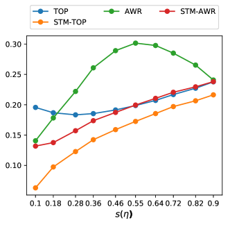
Figure 1: Plots of the estimation error $\|\widehat{A}-A(\eta)\|_{1}/K$ for $\eta\in\{0,0.1,0.2,\ldots,0.9\}$.

6.2 Semi-synthetic data

We evaluate two real-world datasets, a corpus of NIPs articles and a corpus of New York Times (NYT) articles (Dheeru and Karra Taniskidou, 2017). Following (Arora et al., 2013),

1. We removed common stopping words and rare words occurring in less than 150 documents.

2. For each preprocessed dataset, we apply LDA with $K=100$ and obtain an estimated word-topic matrix $A^{(0)}$.

3. For each document $i\in[n]$, we generate the topics $W_{i}$ from a specified distribution.

4. We sample $N$ words from Multinomial${}_{p}(N;A^{(0)}W)$.

6.2.1 NIPs corpus

After this preprocessing stop, the NIPs dataset consists of $n=1,500$ documents with dictionary size $p=1,253$ and mean document length $847$.

1. We set $N=850$ and vary $n\in\{2000,4000,6000,8000,10000\}$ for generating semi-synthetic data.

2. While the estimated $A^{(0)}$ from LDA does not have exact zero entries, we calculate the approximate sparsity level of $A$ by

   $$\textbf{sparsity}={1\over pK}\sum_{j=1}^{p}\sum_{k=1}^{K}1{\left\{A_{jk}\geq 10^{-3}p^{-1}\right\}}\approx 0.696.$$ (30)

   The calculated sparsity indicates that the posterior $A^{(0)}$ from LDA has many entries close to $0$.

3. As in Arora et al. (2013), we manually add $|I_{k}|=m$ anchor words for each topic with $m\in\{1,5\}$. After adding $m$ anchor words, we re-normalize the columns to obtain $A^{(m)}$.

4. The columns of $W$ are generated from the symmetric Dirichlet distribution with parameter 0.03. We sample $N$ words from Multinomial${}_{p}(N;A^{(m)}W)$.

For each combination of $n$ and $m$, we generate $20$ datasets and the average estimation errors $\|\widehat{A}-A\|_{1}/K$ of different algorithms are shown in Figure 2. The bars represent the standard deviations across 20 repetitions. Again, LDA, AWR and STM-AWR are given the correct $K$, while TOP and STM-TOP estimate $K$.

Conclusion. STM-TOP has best overall performance and STM-AWR has the second best result. LDA is dominated by all other algorithms, although increasing the number of iterations might boost the performance of LDA. Both STM-TOP and TOP have better performance when one has more anchor words.

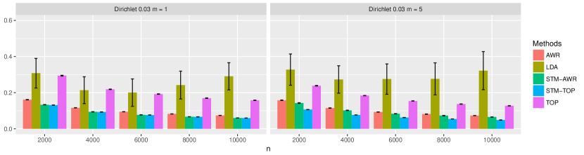
Figure 2: Plots of the estimation errors $\|\widehat{A}-A\|_{1}/K$

We also investigate the effect of the correlation among topics on the estimation of $A$. Following Arora et al. (2013), we simulate $W$ from a log-normal distribution with block diagonal covariance matrix and different within-block correlation. To construct the block diagonal covariance structure, we divide 100 topics into 10 groups. For each group, the off-diagonal elements of the covariance matrix of topics is set to $\rho$, while the diagonal entries are set to 1. The parameter $\rho\in\{0.03,0.3\}$ reflects the magnitude of correlation among topics. We take the case $m=1$ and the estimation errors of the algorithms are shown in Figure 3.

Conclusion. STM-TOP has the best performance in all settings. As long as the number of documents $n$ is large, STM-AWR is more robust to the correlation among topics than AWR. LDA and AWR are comparable.

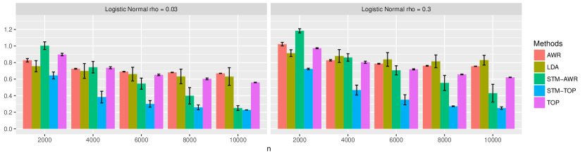
Figure 3: Plots of the estimation errors $\|\widehat{A}-A\|_{1}/K$ for $\rho=0.03$ and $\rho=0.3$.

Finally, we report the running times of the various algorithms in Table 1. As one can see, LDA is the slowest and does not scale well with $n$. On the other hand, TOP is the fastest and the other three algorithms (AWR, STM-AWR and STM-TOP) have comparable running times.

Table 1: Running time (seconds) of different algorithms.

	TOP	STM-TOP	AWR	STM-AWR	LDA
n = 2000	35.2	614.3	393.8	500.7	1918.7
n = 4000	32.8	611.2	447.0	466.2	3724.5
n = 6000	41.8	610.9	455.0	416.7	5616.6
n = 8000	44.7	605.1	458.4	463.5	7358.8
n = 10000	52.0	609.0	482.8	517.9	9130.6

6.2.2 New York Times (NYT) dataset

After the same preprocessing step, the NYT dataset cotains $n=299,419$ documents with dictionary size $p=3,079$ and mean document length $210$. We choose $N=300$ and vary $n\in\{30000,40000,\ldots,70000\}$. The estimated $A^{(0)}$ from LDA has $\textbf{sparsity}\approx 0.679$ calculated from (30). As in the NIPs corpus earlier, we manually add $|I_{k}|=m\in\{1,5\}$ anchor words per topic. For each $m$ and $n$, we generate $20$ datasets where columns of $W$ are generated from the symmetric Dirichlet distribution with parameter $0.03$. The average estimation errors $\|\widehat{A}-A\|_{1}/K$ are shown in Figure 4. We also study the effect of correlation among topics on the estimation errors for the case $m=1$ and with the columns of $W$ generated from the log-normal distribution with block diagonal correlation and $\rho=\{0.1,0.3\}$. The result is shown in Figure 5.

Conclusion. From Figure 4, in the presence of anchor words, we see that STM-TOP has the best overall performance and STM-AWR outperforms AWR. The errors of STM-TOP and TOP decrease if more anchor words are introduced. In Figure 5, STM-TOP outperforms the other algorithms in all cases. TOP has the second best performance while the other three algorithms are comparable.

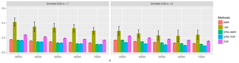
Figure 4: Plots of the estimation errors $\|\widehat{A}-A\|_{1}/K$

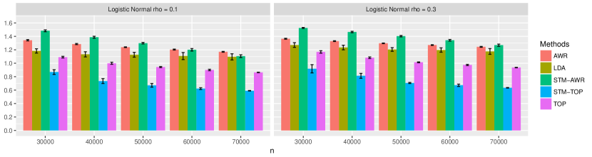
Figure 5: Plots of the estimation errors $\|\widehat{A}-A\|_{1}/K$ for $\rho=0.1$ and $\rho=0.3$.

7 Conclusion

We have studied estimation of the word-topic matrix $A$ when it is possibly entry-wise sparse and the number of topics $K$ is unknown, under the separability condition. A new minimax lower bound of $\|\widehat{A}-A\|_{1}$ is derived and a computationally efficient procedure (STM) for estimating $A$ is proposed. The estimator provably achieves the minimax lower bound (modulo a logarithmic factor) and adapts to the unknown sparsity. Extensive simulations corroborate the superior performance of our new estimation procedure in tandem with the existing algorithm in Bing et al. (2018) for selecting anchor words.

A Proofs

The proofs rely on some lemmas in Bing et al. (2018). For the reader’s convenience, we restate them in Section A.2 and use similar notations for simplicity.

A.1 Notations and two useful expressions

From the topic model specifications, the matrices $\Pi$, $A$ and $W$ are all scaled as

$$\sum_{j=1}^{p}\Pi_{ji}=1,\quad\sum_{j=1}^{p}A_{jk}=1,\quad\sum_{k=1}^{K}W_{ki}=1$$ (31)

for any $1\leq j\leq p$, $1\leq i\leq n$ and $1\leq k\leq K$. In order to adjust their scales properly, we denote

$$m_{j}=p\max_{1\leq i\leq n}\Pi_{ji},~{}~{}\mu_{j}={p\over n}\sum_{i=1}^{n}\Pi_{ji},~{}~{}\alpha_{j}=p\max_{1\leq k\leq K}A_{jk},~{}~{}\gamma_{k}={K\over n}\sum_{i=1}^{n}W_{ki},$$ (32)

so that

$$\sum_{k=1}^{K}\gamma_{k}=K,\qquad\sum_{j=1}^{p}\mu_{j}=p.$$ (33)

Recall that $\rho_{j}=\alpha_{j}/\underline{\alpha}_{L}$ and $\widetilde{s}_{J}:=\sum_{j\in L^{c}}\rho_{j}s_{j}$. We define

$${\widehat{\mu}_{j}\over p}={1\over n}\sum_{t=1}^{n}X_{jt},\qquad\text{for all }1\leq j\leq p.$$ (34)

We write $d:=n\vee p$ throughout the proof. Finally, note that Assumption 3 implies $K<n$.

From model specifications (31) and (32), we derive three useful facts that are later repeatedly invoked.

• For any $j\in[p]$, by using (32),

  $$\mu_{j}={p\over n}\sum_{i=1}^{n}\Pi_{ji}={p\over n}\sum_{i=1}^{n}\sum_{k=1}^{K}A_{jk}W_{ki}={p\over K}\sum_{k=1}^{K}A_{jk}\gamma_{k}~{}~{}\Rightarrow~{}~{}{p\over K}\sum_{k=1}^{K}A_{jk}\cdot\underline{\gamma}\leq\mu_{j}\leq\alpha_{j}.$$ (35)

  In particular, for any $j\in I_{k}$ with any $k\in[K]$,

  $$\mu_{j}={p\over n}\sum_{i=1}^{n}\sum_{k=1}^{K}A_{jk}W_{ki}={p\over K}A_{jk}\gamma_{k}\overset{(\ref{def_uag})}{=}{\alpha_{j}\gamma_{k}\over K}.$$ (36)

• For any $j\in[p]$,

  $$m_{j}\overset{(\ref{def_uag})}{=}{p}\max_{1\leq i\leq n}\Pi_{ji}={p}\max_{1\leq i\leq n}\sum_{k=1}^{K}A_{jk}W_{ki}\leq p\max_{1\leq k\leq K}A_{jk}\overset{(\ref{def_uag})}{=}\alpha_{j}~{}~{}\Rightarrow~{}~{}\mu_{j}\leq m_{j}\leq\alpha_{j},$$ (37)

  by using $0\leq W_{ki}\leq 1$ and $\sum_{k}W_{ki}=1$ for any $k\in[K]$ and $i\in[n]$.

• For any $j\in[p]$ and $k\in[K]$, define

  $$\psi_{jk}=\sum_{a=1}^{K}A_{ja}C_{ak}\text{ with }C=n^{-1}WW^{\top}.$$ (38)

  We have

  $$\sum_{j=1}^{p}\psi_{jk}=\sum_{j=1}^{p}\sum_{a=1}^{K}A_{ja}C_{ak}=\sum_{a=1}^{K}C_{ak}={1\over n}\sum_{t=1}^{n}\sum_{a=1}^{K}W_{kt}W_{at}\overset{(\ref{orig_sum_to_one})}{=}{1\over n}\sum_{t=1}^{n}W_{kt}\overset{(\ref{def_uag})}{=}{\gamma_{k}\over K}.$$ (39)

A.2 Useful results from Bing et al. (2018)

Let $\varepsilon_{ji}:=X_{ji}-\Pi_{ji}$, for $1\leq i\leq n$ and $1\leq j\leq p$ and assume $N_{1}=\ldots=N_{n}=N$ for ease of presentation since similar results for different $N$ can be derived by using the same arguments.

Lemma 8

With probability $1-2d^{-1}$, we have

$${1\over n}\left|\sum_{i=1}^{n}\varepsilon_{ji}\right|>2{\sqrt{\mu_{j}\log(d)\over npN}}+{4\log(d)\over nN},\quad\text{uniformly in $1\leq j\leq p$.}$$ (40)

If $\min_{1\leq j\leq p}\mu_{j}/p\geq\log(d)/(nN)$ holds, with probability $1-2d^{-1}$,

$${1\over n}\left|\sum_{i=1}^{n}\varepsilon_{ji}\right|\leq 6\sqrt{\mu_{j}\log(d)\over npN},\quad\text{uniformly in $1\leq j\leq p$.}$$

Lemma 9

Recall $\Theta=n^{-1}\Pi\Pi^{\top}$. With probability $1-2d^{-1}$,

$${1\over n}\left|\sum_{i=1}^{n}\Pi_{\ell i}\varepsilon_{ji}\right|\leq{\sqrt{6m_{\ell}\Theta_{j\ell}\log(d)\over npN}}+{2m_{\ell}\log(d)\over npN},\quad\text{uniformly in $1\leq j,\ell\leq p$.}$$

Lemma 10

If $\min_{1\leq j\leq p}\mu_{j}/p\geq 2\log(d)/(3N)$, then with probability $1-4d^{-1}$,

$${1\over n}\left|\sum_{i=1}^{n}\left(\varepsilon_{ji}\varepsilon_{\ell i}-\mathbb{E}[\varepsilon_{ji}\varepsilon_{\ell i}]\right)\right|\leq 12\sqrt{6}\sqrt{\Theta_{j\ell}+{(\mu_{j}+\mu_{\ell})\log(d)\over pN}}\sqrt{\log^{3}(d)\over nN^{2}}+4d^{-3},$$

holds, uniformly in $1\leq j,\ell\leq p$.

Lemma 11

Assume model (4) and

$$\min_{1\leq j\leq p}{1\over n}\sum_{i=1}^{n}\Pi_{ji}\geq{c\log(d)\over nN}$$ (41)

for some sufficiently large constant $c>0$. With probability greater than $1-O(d^{-1})$,

$$|\widehat{\Theta}_{j\ell}-\Theta_{j\ell}|\leq c_{0}\eta_{j\ell},\qquad|\widehat{R}_{j\ell}-R_{j\ell}|\leq c_{1}\delta_{j\ell},\quad\text{ for all $1\leq j,\ell\leq p$}$$

for some constant $c_{0},c_{1}>0$, where

$$\eta_{j\ell} =\sqrt{\Theta_{j\ell}\log(d)\over nN}\sqrt{{m_{j}+m_{\ell}\over p}\vee{\log^{2}(d)\over N}}+{(m_{j}+m_{\ell})\over p}{\log(d)\over nN}$$

$$\qquad+\sqrt{\log^{4}(d)\over nN^{3}}\sqrt{{\mu_{j}+\mu_{\ell}\over p}\vee{\log(d)\over N}}$$ (42)

and

$$\delta_{j\ell}:={p^{2}\eta_{j\ell}\over\mu_{j}\mu_{\ell}}+{p^{2}\Theta_{j\ell}\over\mu_{j}\mu_{\ell}}\left(\sqrt{p\over\mu_{j}}+\sqrt{p\over\mu_{\ell}}\right)\sqrt{\log(d)\over nN}.$$ (43)

A.3 Proof of Theorem 1 in Section 2

We first choose $\{I_{1},\ldots,I_{K}\}$ such that $||I_{k}|-|I_{k^{\prime}}||\leq 1$ for any $k,k^{\prime}\in[K]$. This also implies $|I_{k}|\leq 2|I|/K$. Further choose the integer set $\{g_{1},\ldots,g_{K}\}$ such that $\sum_{k=1}^{K}g_{k}=s_{J}$ and $|g_{k}-g_{k^{\prime}}|\leq 1$ for any $k,k^{\prime}\in[K]$, further implying $g_{k}\leq 2s_{J}/K$. We first choose $A^{(0)}$. Let

$$\widetilde{A}^{(0)}=\begin{bmatrix}\bm{1}_{|I_{1}|}&&&\\ &\bm{1}_{|I_{2}|}&&\\ &&\ddots&\\ &&&\bm{1}_{|I_{K}|}\\ \widetilde{\bm{1}}_{g_{1}}&\widetilde{\bm{1}}_{g_{2}}&\cdots&\widetilde{\bm{1}}_{g_{K}}\end{bmatrix}$$ (44)

where, for any $k\in[K]$, $\widetilde{\bm{1}}_{g_{k}}=\bm{1}_{g_{k}}$ if $g_{k}=|J|$ and $\widetilde{\bm{1}}_{g_{k}}=(\bm{1}_{g_{k}}^{\top},0^{\top})^{\top}$ otherwise. We then set

$$A^{(0)}=\widetilde{A}^{(0)}\begin{bmatrix}{1\over|I_{1}|+g_{1}}&&&\\ &{1\over|I_{2}|+g_{2}}&&\\ &&\ddots&\\ &&&{1\over|I_{K}|+g_{K}}\\ \end{bmatrix}.$$

We start by constructing a set of “hypotheses” of $A$. Assume $|I_{k}|+g_{k}$ is even for $1\leq k\leq K$. Let

$$\mathcal{M}:=\{0,1\}^{(|I|+s_{J})/2}.$$

Following the Varshamov-Gilbert bound in Lemma 2.9 in Tsybakov (2009), there exists $w^{(j)}\in\mathcal{M}$ for $j=0,1,\ldots,T$, such that

$$\left\|w^{(i)}-w^{(j)}\right\|_{1}\geq{|I|+s_{J}\over 16},\quad\text{for any }0\leq i\neq j\leq T,$$ (45)

with $w^{(0)}=0$ and

$$\log(T)\geq{\log(2)\over 16}(|I|+s_{J}).$$ (46)

For each $w^{(j)}\in\mathcal{M}$, we divide it into $K$ chunks as $w^{(j)}=\left(w^{(j)}_{1},w^{(j)}_{2},\ldots,w^{(j)}_{K}\right)$ with $w^{(j)}_{k}\in\mathbb{R}^{(|I_{k}|+g_{k})/2}$. For each $w^{(j)}_{k}$, we write $\widetilde{w}^{(j)}_{k}\in\mathbb{R}^{p}$ as its augumented counterpart such that $[\widetilde{w}^{(j)}_{k}]_{S_{k}}=[w^{(j)}_{k},-w^{(j)}_{k}]$ and $[\widetilde{w}^{(j)}_{k}]_{\ell}=0$ for any $\ell\notin S_{k}$, where $S_{k}:=\textrm{supp}(A^{(0)}_{k})$. For $1\leq j\leq T$, we choose $A^{(j)}$ as

$$A^{(j)}=A^{(0)}+\gamma\begin{bmatrix}\widetilde{w}^{(j)}_{1}&\cdots&\widetilde{w}^{(j)}_{K}\end{bmatrix}$$ (47)

with

$$\gamma=\sqrt{\log(2)\over 4^{5}(1+c_{0})}\sqrt{K^{2}\over nN(|I|+s_{J})}$$ (48)

for some constant $c_{0}>0$. Under $|I|+s_{J}\leq nN$, it is easy to verify that $A^{(j)}\in\mathcal{A}(|I|,s_{J})$ for all $0\leq j\leq T$.

In order to apply Theorem 2.5 in Tsybakov (2009), we need to check the following conditions:

• $\textrm{KL}(\mathbb{P}_{A^{(j)}},\mathbb{P}_{A^{(0)}})\leq\log(T)/16$, for each $i=1,\ldots,T$.

• $\|A^{(i)}-A^{(j)}\|_{1}\geq c_{1}K\sqrt{(|I|+s_{J})/(nN)}$, for $0\leq i<j\leq T$ and some constant $c_{1}>0$.

We first show part (a). Fix $1\leq j\leq T$ and choose $D^{(j)}=A^{(j)}W^{0}$ where $W^{0}$ is defined in (8). Let $m_{k}$ be the set such that $|m_{k}|=n_{k}$ and $W_{i}^{0}=e_{k},$ for all $i\in m_{k}$ and $k\in[K]$. Since $|I_{k}|+g_{k}\leq 2(|I|+s_{J})/K$, it follows that

$$D^{(0)}_{\ell i}=\sum_{k=1}^{K}A^{(0)}_{\ell k}W_{ki}^{0}=\left\{\begin{array}[]{ll}1/(|I_{k}|+g_{k})\geq 2^{-1}K/(|I|+s_{J}),&\text{ if }\ell\in S_{k},i\in m_{k},k\in[K]\\ 0,&\text{ otherwise}\end{array}\right..$$ (49)

for any $i\in[n]$ and $\ell\in[p]$. Similarly, we have

$$\left|D^{(j)}_{\ell i}-D^{(0)}_{\ell i}\right|=\gamma\left|\sum_{k=1}^{K}[\widetilde{w}_{k}^{(j)}]_{\ell}W_{ki}^{0}\right|\leq\left\{\begin{array}[]{ll}\gamma,&\text{ if }\ell\in S_{k},i\in m_{k},k\in[K]\\ 0,&\text{ otherwise}\end{array}\right..$$ (50)

Thus, by $|I|+s_{J}\leq nN$, we have

$$\max_{(\ell,i)\in\mathcal{T}^{c}}{|D^{(j)}_{\ell i}-D_{\ell i}^{(0)}|\over D_{\ell i}^{(0)}}\leq 2\gamma{|I|+s_{J}\over K}<1,\qquad\text{for any $1\leq j\leq T$}$$

where $\mathcal{T}:=\{(\ell,i)\in[p]\times[n]:D_{\ell i}^{(0)}=0\}$ and $\mathcal{T}^{c}:=[p]\times[n]\setminus\mathcal{T}$. Observe that $D^{(j)}_{\ell i}=0$ for any $(\ell,i)\in\mathcal{T}$ and $1\leq j\leq T$, and invoke Lemma 12 to get

$$\textrm{KL}(\mathbb{P}_{A^{(j)}},\mathbb{P}_{A^{(0)}}) ~{}\leq~{}\left(1+c_{0}\right)N\sum_{(\ell,i)\in\mathcal{T}}{|D^{(j)}_{\ell i}-D^{(0)}_{\ell i}|^{2}\over D^{(0)}_{\ell i}}$$

$$~{}\leq~{}\left(1+c_{0}\right)N\sum_{k=1}^{K}\sum_{i\in m_{k}}\sum_{\ell\in S_{k}}\gamma^{2}(|I_{k}|+g_{k})$$

$$~{}=~{}\left(1+c_{0}\right)N\sum_{k=1}^{K}\sum_{i\in m_{k}}\gamma^{2}(|I_{k}|+g_{k})^{2}\qquad(\text{by }|S_{k}|=|I_{k}|+g_{k})$$

$$~{}\leq~{}4\left(1+c_{0}\right)Nn\gamma^{2}{(|I|+s_{J})^{2}\over K^{2}}$$

$$\overset{(\ref{eq_T})}{\leq}{1\over 16}\log T.$$

The second inequality uses (49) and (50) and the fourth line uses $|I_{k}|+g_{k}\leq 2(|I|+s_{J})/K$. This verifies (a).

To show (b), (47) yields

$$\|A^{(j)},A^{(\ell)}\|_{1} =\sum_{k=1}^{K}\left\|A^{(j)}_{\cdot k}-A^{(\ell)}_{\cdot k}\right\|_{1}$$

$$=2\gamma\sum_{k=1}^{K}\left\|w^{(j)}_{k}-w^{(\ell)}_{k}\right\|_{1}$$

$$=2\gamma\left\|w^{(j)}-w^{(\ell)}\right\|_{1}$$

$$\overset{(\ref{eq_w})}{\geq}{\gamma\over 8}(|I|+s_{J}).$$

After we plug this into the expression of $\gamma$, we obtain (b). Invoking (Tsybakov, 2009, Theorem 2.5) concludes the proof when $|I_{k}|+g_{k}$ is even for all $k\in[K]$. The complementary case is easy to derive with slight modifications. Specifically, denote by $\mathcal{S}_{odd}:=\{1\leq k\leq K:|I_{k}|+g_{k}\text{ is odd}\}$. Then we change $\mathcal{M}:=\{0,1\}^{Card}$ with

$$Card=\sum_{k\in\mathcal{S}_{odd}}{|I_{k}|+g_{k}-1\over 2}+\sum_{k\in\mathcal{S}_{odd}^{c}}{|I_{k}|+g_{k}\over 2}.$$

For each $w^{(j)}$, we write it as $w^{(j)}=(w^{(j)}_{1},\ldots,w^{(j)}_{K})$ and each $w^{(j)}_{k}$ has length $(|I_{k}|+g_{k}-1)/2$ if $k\in\mathcal{S}_{odd}$ and $(|I_{k}|+g_{k})/2$ otherwise. We then construct $A^{(j)}_{k}=A_{k}^{(0)}+\gamma\widetilde{w}^{(j)}_{k}$ where $\widetilde{w}^{(j)}_{k}\in\mathbb{R}^{p}$ is the same augumented ccounterpart of $w^{(j)}_{k}$. The result follows from the same arguments and the proof is complete.  

The upper bound of Kullback-Leibler divergence between two multinomial distributions is studied in (Ke and Wang, 2017, Lemma 6.7). We use the following modification of their bound.

Lemma 12

Let $D$ and $D^{\prime}$ be two $p\times n$ matrices such that each column of them is a weight vector. Under model (4), let $\mathbb{P}$ and $\mathbb{P}^{\prime}$ be the probability measures associated with $D$ and $D^{\prime}$, respectively. Let $\mathcal{T}$ be the set such that

$$\mathcal{T}:=\left\{(j,i)\in[p]\times[n]:D_{ji}=D^{\prime}_{ji}=0\right\}$$

Let $\mathcal{T}^{c}:=([p]\times[n])\setminus\mathcal{T}$ and

$$\eta=\max_{(j,i)\in\mathcal{T}^{c}}{|D^{\prime}_{ji}-D_{ji}|\over D_{ji}}$$

and assume $\eta<1$. There exists a universal constant $c_{0}>0$ such that

$$\textrm{KL}(\mathbb{P}^{\prime},\mathbb{P})\leq(1+c_{0}\eta)N\sum_{(j,i)\in\mathcal{T}^{c}}{|D^{\prime}_{ji}-D_{ji}|^{2}\over D_{ji}}.$$

Proof  With the convention that $0/0=1$, we have

$$KL(\mathbb{P}^{\prime},\mathbb{P})=N\sum_{i=1}^{n}\sum_{j=1}^{p}D^{\prime}_{ji}\log\left(D^{\prime}_{ji}\over D_{ji}\right)=N\sum_{(j,i)\in\mathcal{T}^{c}}D^{\prime}_{ji}\log\left(1+\eta_{ji}\right).$$

Then the proof follows by the same arugments in Ke and Wang (2017).  

A.4 Proofs of Section 4

We first give the proof of Lemma 3 and then prove our main Theorem 2.

A.4.1 Proof of Lemma 3

From (18), we have

$$\widehat{M}_{ab}={1\over|L_{a}||L_{b}|}\sum_{i\in L_{a},j\in L_{b}}\widehat{R}_{ij}.$$

Further notice that

$${1\over|L_{a}||L_{b}|}\sum_{i\in L_{a},j\in L_{b}}R_{ij}=M_{ab}.$$

Using the fact that $\|Q\|_{\rm{\rm{\rm{op}}}}\leq\|Q\|_{{\infty,1}}$ for any symmetric matrix $Q$, yields

$$\|\widehat{M}-M\|_{\rm{\rm{\rm{op}}}} \leq\|\widehat{M}-M\|_{\infty,1}$$

$$=\max_{1\leq k\leq K}\sum_{a=1}^{K}\left|{1\over|L_{a}||L_{b}|}\sum_{i\in L_{a},j\in L_{b}}(\widehat{R}_{ij}-R_{ij})\right|$$

$$\leq\max_{1\leq k\leq K}\max_{i\in L_{k}}\sum_{a=1}^{K}\max_{j\in L_{a}}|\widehat{R}_{ij}-R_{ij}|.$$

Invoking Lemma 11 for all $i,j\in L$ under condition (24), with probability $1-O(d^{-1})$, we have

$$\|\widehat{M}-M\|_{\rm{\rm{\rm{op}}}} \leq\max_{1\leq k\leq K}\max_{i\in L_{k}}\sum_{a=1}^{K}\max_{j\in L_{a}}\delta_{ij}.$$

The result follows by invoking Lemma 14.  

A.4.2 Proof of Theorem 2

As our estimation procedure uses a thresholding step in (19), we first define

$$T:=\left\{j\in L^{c}:{1\over n}\sum_{i=1}^{n}\Pi_{ji}<{\log(d)\over nN}\right\},\quad\widehat{T}:=\left\{j\in L^{c}:{1\over n}\sum_{i=1}^{n}X_{ji}<{7\log(d)\over nN}\right\}$$ (51)

and write $T^{c}:=[p]\setminus T$ and $\widehat{T}^{c}:=[p]\setminus\widehat{T}$.
Recall that our final estimator $\widehat{A}$ is obtained by normalizing $\widehat{\bar{B}}=D_{X}\widehat{B}$ to unit column sums with $D_{X}=\textrm{diag}\left({\widehat{u}_{1}/p},\ldots,{\widehat{u}_{p}/p}\right)$ where $\widehat{u}_{j}/p$ is defined in (34) for $1\leq j\leq p$. For any $j\in[p]$ and $k\in[K]$, we have

$$\widehat{A}_{jk}-A_{jk}={\widehat{\bar{B}}_{jk}\over\|\widehat{\bar{B}}_{k}\|_{1}}-{\bar{B}_{jk}\over\|\bar{B}_{k}\|_{1}}$$

where $\bar{B}=D_{\Pi}B$. Summing over $1\leq j\leq p$ yields

$$\|\widehat{A}_{k}-A_{k}\|_{1} =\sum_{j=1}^{p}\left|{\widehat{\bar{B}}_{jk}\over\|\widehat{\bar{B}}_{k}\|_{1}}-{\widehat{\bar{B}}_{jk}\over\|\bar{B}_{k}\|_{1}}+{\widehat{\bar{B}}_{jk}-\bar{B}_{jk}\over\|\bar{B}_{k}\|_{1}}\right|$$

$$\leq{|\|\bar{B}_{k}\|_{1}-\|\widehat{\bar{B}}_{k}\|_{1}|\over\|\bar{B}_{k}\|_{1}}+{\|\widehat{\bar{B}}_{k}-\bar{B}_{k}\|_{1}\over\|\bar{B}_{k}\|_{1}}$$

$$\leq{2\|\widehat{\bar{B}}_{k}-\bar{B}_{k}\|_{1}\over\|\bar{B}_{k}\|_{1}}$$

$$={2K\over\gamma_{k}}\|\widehat{\bar{B}}_{k}-\bar{B}_{k}\|_{1}.$$

In the last equality, we use

$$\|\bar{B}_{k}\|_{1}=\sum_{j=1}^{p}A_{jk}{1\over n}\sum_{t=1}^{n}W_{kt}={\gamma_{k}\over K},$$

by observing that $\bar{B}=D_{\Pi}B=AD_{W}$. Further recall that $\widehat{\bar{B}}_{jk}=\widehat{\mu}_{j}\widehat{B}_{jk}/p$ for $j\in[p]$ and $\widehat{B}_{j\cdot}=0$ for any $j\in\widehat{T}$. We have

$$\|\widehat{A}_{k}-A_{k}\|_{1} ={2K\over\gamma_{k}}\sum_{j=1}^{p}\left|{\widehat{\mu}_{j}\over p}\widehat{B}_{jk}-{\mu_{j}\over p}B_{jk}\right|$$

$$\leq{2K\over\gamma_{k}}\sum_{j=1}^{p}\left\{\widehat{B}_{jk}{|\widehat{\mu}_{j}-\mu_{j}|\over p}+{\mu_{j}\over p}|\widehat{B}_{jk}-B_{jk}|\right\}$$

$$={2K\over\gamma_{k}}\left\{\sum_{j\in\widehat{T}^{c}}\left(\widehat{B}_{jk}{|\widehat{\mu}_{j}-\mu_{j}|\over p}+{\mu_{j}\over p}|\widehat{B}_{jk}-B_{jk}|\right)+\sum_{j\in\widehat{T}}{\mu_{j}B_{jk}\over p}\right\}$$

$$={2K\over\gamma_{k}}\sum_{j\in\widehat{T}^{c}}\left(\widehat{B}_{jk}{|\widehat{\mu}_{j}-\mu_{j}|\over p}+{\mu_{j}\over p}|\widehat{B}_{jk}-B_{jk}|\right)+2\sum_{j\in\widehat{T}}A_{jk}.$$

We use $A_{jk}=(\mu_{j}/p)B_{jk}(K/\gamma_{k})$ in the last line. Summing over $1\leq k\leq K$ gives

$$\|\widehat{A}-A\|_{1} \leq{2K\over\underline{\gamma}}\sum_{j\in\widehat{T}^{c}}\left({|\widehat{\mu}_{j}-\mu_{j}|\over p}+{\mu_{j}\over p}\|\widehat{B}_{j\cdot}-B_{j\cdot}\|_{1}\right)+2\sum_{j\in\widehat{T}}\|A_{j\cdot}\|_{1}$$

$$={2K\over\underline{\gamma}}\left\{\sum_{j\in\widehat{T}^{c}}{|\widehat{\mu}_{j}-\mu_{j}|\over p}+\sum_{j\in\widehat{T}^{c}\setminus L}{\mu_{j}\over p}\|\widehat{B}_{j\cdot}-B_{j\cdot}\|_{1}\right\}+2\sum_{j\in\widehat{T}}\|A_{j\cdot}\|_{1}.$$

We use $\|\widehat{B}_{jk}\|_{1}=1$ in the first line and the fact $\widehat{B}_{j\cdot}=B_{j\cdot}$ for all $j\in L$ in the second line.

Next, we study the three terms on the right hand side. To bound the first term, we observe that

$$\mathbb{P}\{T\subseteq\widehat{T}\}=\mathbb{P}\{\widehat{T}^{c}\subseteq T^{c}\}=1-2d^{-1},$$

by Lemma 13. This fact, the second part of Lemma 8 and the inequality

$$\min_{j\in T^{c}}{\mu_{j}\over p}\geq{\log(d)\over nN}.$$ (52)

yield

$$\mathbb{P}\left\{\sum_{j\in\widehat{T}^{c}}{|\widehat{\mu}_{j}-\mu_{j}|\over p}\leq\sum_{j\in T^{c}}{|\widehat{\mu}_{j}-\mu_{j}|\over p}\leq\sum_{j\in T^{c}}6\sqrt{\mu_{j}\log(d)\over npN}\right\}\geq 1-4d^{-1}.$$

Further, the Cauchy-Schwarz inequality and $\sum_{j\in T^{c}}\mu_{j}/p\leq\sum_{j=1}^{p}\mu_{j}/p=1$ yield

$$\mathbb{P}\left\{\sum_{j\in\widehat{T}^{c}}{|\widehat{\mu}_{j}-\mu_{j}|\over p}\leq 6\sqrt{|T^{c}|\log(d)\over nN}\leq 6\sqrt{p\log(d)\over nN}\right\}\geq 1-4d^{-1}.$$ (53)

To bound the third term, Lemma 13 yields

$$\mathbb{P}\left\{\sum_{j\in\widehat{T}}\|A_{j\cdot}\|_{1}\leq{20K|\widehat{T}|\log(d)\over\underline{\gamma}nN}\leq{20Kp\log(d)\over\underline{\gamma}nN}\right\}\geq 1-2d^{-1}.$$ (54)

The proof of the upper bound for the second term is more involved. We work on the intersection of the event $\{\widehat{T}^{c}\subseteq T^{c}\}$ with

$$\mathcal{E}_{M}:=\left\{\lambda_{\min}(\widehat{M}+\lambda\bm{I}_{K})\geq\lambda_{\min}(M)+\lambda-\|\widehat{M}-M\|_{\rm{\rm{op}}}\geq\lambda_{\min}(M)\right\}$$

to establish an upper bound for

$$\sum_{j\in T^{c}\setminus L}{\mu_{j}\over p}\|\widehat{B}_{j\cdot}-B_{j\cdot}\|_{1}.$$

Lemma 3 and the choice of $\lambda$ guarantee $\mathbb{P}(\mathcal{E}_{M})=1-O(d^{-1})$. Pick any $j\in T^{c}\setminus L$ and recall that $\widehat{B}_{j\cdot}$ is estimated via (20). Starting with

$$\widehat{B}_{j\cdot}^{\top}(\widehat{M}+\lambda\bm{I}_{K})\widehat{B}_{j\cdot}-2\widehat{B}_{j\cdot}^{\top}\widehat{h}^{(j)}\leq B_{j\cdot}^{\top}(\widehat{M}+\lambda\bm{I}_{K})^{-1}B_{j\cdot}-2B_{j\cdot}^{\top}\widehat{h}^{(j)},$$

standard arguments yield

$$(\Delta^{(j)})^{\top}(\widehat{M}+\lambda\bm{I}_{K})\Delta^{(j)} \leq 2\left|(\Delta^{(j)})^{\top}(\widehat{h}^{(j)}-\widehat{M}B_{j\cdot}-\lambda B_{j\cdot})\right|$$

$$\leq 2\left\{|(\Delta^{(j)})^{\top}(\widehat{h}^{(j)}-h^{(j)})|+|(\Delta^{(j)})^{\top}(h^{(j)}-\widehat{M}B_{j\cdot})|+\lambda\|\Delta^{(j)}\|\|B_{j\cdot}\|\right\}$$

by writing $\Delta^{(j)}:=\widehat{B}_{j\cdot}-B_{j\cdot}$. Hence, on the event $\mathcal{E}_{M}$, we have

$$\|\Delta^{(j)}\| \leq{2\over\lambda_{\min}(M)}\left\{{|(\Delta^{(j)})^{\top}(\widehat{h}^{(j)}-h^{(j)})|\over\|\Delta^{(j)}\|}+{|(\Delta^{(j)})^{\top}(h^{(j)}-\widehat{M}B_{j\cdot})|\over\|\Delta^{(j)}\|}+\lambda\|B_{j\cdot}\|\right\}.$$ (55)

Let $s_{j}=\|B_{j\cdot}\|_{0}$ and $S_{j}=\textrm{supp}(B_{j\cdot})$. Since

$$0=\|B_{j\cdot}\|_{1}-\|\widehat{B}_{j\cdot}\|_{1}=\|B_{jS_{j}}\|_{1}-\|\widehat{B}_{jS_{j}}\|_{1}-\|\widehat{B}_{jS_{j}^{c}}\|_{1}\leq\|\Delta^{(j)}_{S_{j}}\|_{1}-\|\Delta^{(j)}_{S_{j}^{c}}\|_{1},$$

we have

$$\|\Delta^{(j)}\|_{1}\leq 2\|\Delta^{(j)}_{S_{j}}\|_{1}\leq 2\sqrt{s_{j}}\|\Delta^{(j)}_{S_{j}}\|\leq 2\sqrt{s_{j}}\|\Delta^{(j)}\|.$$ (56)

Combination of (56) with (55) gives

$$\sum_{j\in T^{c}\setminus L}{\mu_{j}\over p}\|\widehat{B}_{j\cdot}-B_{j\cdot}\|_{1}$$

$$\leq 2\sum_{j\in T^{c}\setminus L}{\mu_{j}\over p}\sqrt{s_{j}}\|\Delta^{(j)}\|$$

$$\leq{4\over\lambda_{\min}(M)}\sum_{j\in T^{c}\setminus L}\sqrt{s_{j}}\cdot{\mu_{j}\over p}\left\{{|(\Delta^{(j)})^{\top}(\widehat{h}^{(j)}-h^{(j)})|\over\|\Delta^{(j)}\|}+{|(\Delta^{(j)})^{\top}(h^{(j)}-\widehat{M}B_{j\cdot})|\over\|\Delta^{(j)}\|}+\lambda\|B_{j\cdot}\|\right\}$$ (57)

The results of Lemmas 15 and 16 and the inequality $\lambda_{\min}(M)\geq\lambda_{\min}K^{2}/\overline{\gamma}^{2}$ give

$$\sum_{j\in T^{c}\setminus L}{\mu_{j}\over p}\|\widehat{B}_{j\cdot}-B_{j\cdot}\|_{1}$$

$$\quad\lesssim{\overline{\gamma}^{2}\over K^{2}\lambda_{\min}}\Biggl{\{}\max\left\{s_{J}+|I|-|L|,\widetilde{s}_{J}\right\}\left({K\log(d)\over\underline{\gamma}nN}+\sqrt{p\log^{4}(d)\over\underline{\mu}_{L}nN^{3}}\right)$$

$$\quad+K\sqrt{\max\left\{s_{J}+|I|-|L|,\widetilde{s}_{J}\right\}{\log(d)\over\underline{\gamma}nN}}+\lambda\sum_{j\in T^{c}\setminus L}\sqrt{s_{j}}{\mu_{j}\over p}\|B_{j\cdot}\|\Biggr{\}}.$$ (58)

Finally, (53), (54) and (A.4.2) together imply that

$$\|\widehat{A}-A\|_{1} \lesssim{K\over\underline{\gamma}}\sqrt{p\log(d)\over nN}+{pK\log(d)\over\underline{\gamma}nN}$$

$$\quad+{\overline{\gamma}^{2}\over\underline{\gamma}K\lambda_{\min}}\Biggl{\{}\max\left\{s_{J}+|I|-|L|,\widetilde{s}_{J}\right\}\left({K\log(d)\over\underline{\gamma}nN}+\sqrt{p\log^{4}(d)\over\underline{\mu}_{L}nN^{3}}\right)$$

$$\quad+K\sqrt{\max\left\{s_{J}+|I|-|L|,\widetilde{s}_{J}\right\}{\log(d)\over\underline{\gamma}nN}}+\lambda\sum_{j\in T^{c}\setminus L}\sqrt{s_{j}}{\mu_{j}\over p}\|B_{j\cdot}\|\Biggr{\}}.$$ (59)

holds with probability $1-O(d^{-1})$. After we invoke the result of Lemma 17, the proof of the first result follows. The second result follows by setting $\lambda=0$ in (A.4.2) as

$$\mathbb{P}\left\{\lambda_{\min}(\widehat{M})\geq\lambda_{\min}(M)-\|\widehat{M}-M\|_{\rm{\rm{op}}}\geq c\lambda_{\min}(M)\right\}\geq 1-O(d^{-1}).$$

A.5 Lemmas used in the proof of Theorem 2

Lemma 13

Let $T$ and $\widehat{T}$ be defined in (51). With probability $1-2d^{-1}$, we have $T\subseteq\widehat{T}$ and, for any $1\leq j\leq p$, if

$${1\over n}\sum_{i=1}^{n}X_{ji}<{7\log(d)\over nN},$$

we further have

$$\|A_{j\cdot}\|_{1}\leq{19K\log(d)\over\underline{\gamma}nN}.$$

Proof  Recall that $X_{ji}=\Pi_{ji}+\varepsilon_{ji}$ such that $\widehat{\mu}_{j}/p=\mu_{j}/p+n^{-1}\sum_{i=1}^{n}\varepsilon_{ji}$. We work on the event

$$\mathcal{E}_{1}:=\bigcap_{j=1}^{p}\left\{{1\over n}\left|\sum_{i=1}^{n}\varepsilon_{ji}\right|<2\sqrt{\mu_{j}\log(d)\over npN}+{4\log(d)\over nN}\right\}$$

which holds with probability $1-2d^{-1}$ from Lemma 8. Since, for any $j\in T$,

$${\widehat{u}_{j}\over p}\leq{\mu_{j}\over p}+{|\widehat{\mu}_{j}-\mu_{j}|\over p}\overset{\mathcal{E}_{1}}{<}{\log(d)\over nN}+2\sqrt{\mu_{j}\log(d)\over npN}+{4\log(d)\over nN}<{7\log(d)\over nN},$$

we have $j\in\widehat{T}$, hence $T\subseteq\widehat{T}$.

To prove the second statement, for any $j$ such that $\widehat{u}_{j}/p\leq 7\log(d)/(nN)$, we have

$${\mu_{j}\over p}\leq{\widehat{\mu}_{j}\over p}+{1\over n}\left|\sum_{i=1}^{n}\varepsilon_{ji}\right|<{7\log(d)\over nN}+{1\over n}\left|\sum_{i=1}^{n}\varepsilon_{ji}\right|.$$

For this $j$, since

$$\mathbb{P}\left\{{1\over n}\left|\sum_{i=1}^{n}\varepsilon_{ji}\right|<2\sqrt{\mu_{j}\log(d)\over npN}+{4\log(d)\over nN}\right\}\geq\mathbb{P}(\mathcal{E}_{1})=1-2d^{-1},$$

we have, with probability $1-2d^{-1}$,

$${\mu_{j}\over p}<2\sqrt{\mu_{j}\log(d)\over npN}+{11\log(d)\over nN},$$

which implies $\mu_{j}/p\leq 19\log(d)/(nN)$. The result then follows by using (35).  

Lemma 14

Let $\delta_{ij}$ be defined in (43) for any $i,j\in[p]$. Let $\psi_{jk}$ be defined in (38) for any $j\in[p]$, $k\in[K]$. Under condition (24), we have

$$\max_{1\leq k\leq K}\max_{i\in L_{k}}\sum_{a=1}^{K}\max_{j\in L_{a}}\delta_{ij} \lesssim{K\over\underline{\gamma}}\sqrt{pK\log(d)\over\underline{\mu}_{L}nN}$$

and, for any $k\in[K]$ and $j\in[p]$,

$$\sqrt{p\log(d)\over\underline{\mu}_{L}nN}\max_{i\in L_{k}}\sum_{a=1}^{K}{A_{ja}\gamma_{a}\over K}\max_{\ell\in L_{a}}\delta_{i\ell}\lesssim K\sqrt{\rho_{j}\psi_{jk}\log(d)\over\underline{\gamma}\gamma_{k}nN}+\sqrt{\|A_{j\cdot}\|_{1}}\sqrt{\rho_{j}\log(d)\over\gamma_{k}nN}.$$

For any $j\in[p]$, if

$${1\over n}\sum_{t=1}^{n}\Pi_{jt}\geq{c\log(d)\over nN},$$

for some constant $c>0$, we further have

$${\mu_{j}\over p}\max_{i\in L_{k}}\delta_{ij}\lesssim\left(1+\rho_{j}\right){K\log(d)\over\gamma_{k}nN}+\sqrt{p\log^{4}(d)\over\underline{\mu}_{L}nN^{3}}+{K\over\gamma_{k}}\sqrt{\left(1+\rho_{j}\right){\psi_{jk}\log(d)\over nN}}+\sqrt{{\mu_{j}\over p}{K\log(d)\over\gamma_{k}nN}}.$$

Proof  For any $i\in L_{k}$ and $j\in L_{a}$ with $a,k\in[K]$, we start with the expressions in (11) and (43). Note that (35), (37) and (64) imply

$${m_{i}+m_{j}\over p}\geq{2c_{1}\log^{2}(d)\over p},\quad{\mu_{i}+\mu_{j}\over p}={1\over n}\sum_{t=1}^{n}(\Pi_{it}+\Pi_{jt})\geq{2c_{0}\log(d)\over N}.$$ (60)

Also, using $m_{i}\leq\alpha_{i}$ from (37) and $\mu_{i}=\alpha_{i}\gamma_{k}/K$ from (36), together with

$$\Theta_{ij}={1\over n}\sum_{t=1}^{n}A_{ik}W_{kt}W_{at}A_{ja}=A_{ik}A_{ja}C_{ka}\overset{(\ref{def_alpha_gamma})}{=}{\alpha_{i}\alpha_{j}C_{ka}\over p^{2}},$$ (61)

we obtain

$$\delta_{ij} \lesssim{K^{2}\over\gamma_{k}\gamma_{a}}\Biggl{\{}\sqrt{C_{ka}\left({1\over\alpha_{i}}+{1\over\alpha_{j}}\right){p\log(d)\over nN}}+\left({1\over\alpha_{i}}+{1\over\alpha_{j}}\right){p\log(d)\over nN}$$

$$\qquad+\sqrt{\alpha_{i}\gamma_{k}+\alpha_{j}\gamma_{a}\over\alpha_{i}^{2}\alpha_{j}^{2}}\sqrt{p^{3}\log^{4}(d)\over KnN^{3}}+C_{ka}\left(\sqrt{1\over\alpha_{i}\gamma_{k}}+\sqrt{1\over\alpha_{j}\gamma_{k}}\right)\sqrt{pK\log(d)\over nN}\Biggr{\}}.$$ (62)

Using the Cauchy-Schwarz inequality and the fact that

$$\sum_{a=1}^{K}C_{ka}={1\over n}\sum_{t=1}^{n}\sum_{a=1}^{K}W_{kt}W_{at}={1\over n}\sum_{t=1}^{n}W_{kt}\overset{(\ref{def_alpha_gamma})}{=}{\gamma_{k}\over K},$$ (63)

we further have, after a bit of algebra,

$$\max_{i\in L_{k}}\sum_{a=1}^{K}\max_{j\in L_{a}}\delta_{ij}\lesssim{K^{2}\over\underline{\gamma}}\Biggl{\{}\sqrt{p\log(d)\over\underline{\alpha}_{L}\underline{\gamma}nN}+{pK\log(d)\over\underline{\alpha}_{L}\underline{\gamma}nN}+\sqrt{p\log(d)\over\underline{\alpha}_{L}\underline{\gamma}KnN}+\sqrt{p^{3}K\log^{4}(d)\over\underline{\alpha}_{L}^{3}\underline{\gamma}^{2}nN^{3}}\Biggr{\}}$$

where we also use $\alpha_{i}\geq\underline{\alpha}_{L}$, $\gamma_{a}\geq\underline{\gamma}$. Note that the first term on the right-hand side dominates the other three as

$${pK^{2}\log(d)\over\underline{\alpha}_{L}\underline{\gamma}nN}\leq{1\over c_{0}},\quad{p^{2}K\log^{3}(d)\over\underline{\alpha}_{L}^{2}\underline{\gamma}N^{2}}\leq{p\log^{2}(d)\over c_{0}\underline{\alpha}_{L}N}\leq{1\over c_{0}c_{1}}$$

by using $K<n$ and the following observation from (24),

$${\underline{\alpha}_{L}\over p}\overset{(\ref{eq_m})}{\geq}\min_{i\in L}{m_{i}\over p}\geq{c_{1}\log^{2}(d)\over N},\qquad{\underline{\alpha}_{L}\over pK}\geq{\underline{\alpha}_{L}\underline{\gamma}\over pK}\overset{(\ref{eq_mu_I})}{=}{\underline{\mu}_{L}\over p}\geq{c_{0}\log(d)\over N}.$$ (64)

The first result then follows by using $\underline{\mu}_{L}=\underline{\alpha}_{L}\underline{\gamma}/K$ from (36).

To prove the second result, we argue

$$\sum_{a=1}^{K}{A_{ja}\gamma_{a}\over K}\max_{i\in L_{k},\ell\in L_{a}}\delta_{i\ell}$$

$$\lesssim{K\over\gamma_{k}}\sum_{a=1}^{K}A_{ja}\Biggl{\{}\sqrt{C_{ka}p\log(d)\over\underline{\alpha}_{L}nN}+\sqrt{p^{3}\overline{\gamma}\log^{4}(d)\over K\underline{\alpha}_{L}^{3}nN^{3}}+C_{ka}\sqrt{pK\log(d)\over\underline{\alpha}_{L}\underline{\gamma}nN}+{p\log(d)\over\underline{\alpha}_{L}nN}\Biggr{\}}$$

$$\lesssim{K\over\gamma_{k}}\sum_{a=1}^{K}A_{ja}\Biggl{\{}\sqrt{C_{ka}p\log(d)\over\underline{\alpha}_{L}nN}+C_{ka}\sqrt{pK\log(d)\over\underline{\alpha}_{L}\underline{\gamma}nN}+{p\log(d)\over\underline{\alpha}_{L}nN}\Biggr{\}}$$

$$\leq{K\over\gamma_{k}}\sqrt{\rho_{j}\psi_{jk}K\log(d)\over nN}+K\sqrt{\rho_{j}\psi_{jk}K\log(d)\over\underline{\gamma}\gamma_{k}nN}+\|A_{j\cdot}\|_{1}{pK\log(d)\over\underline{\alpha}_{L}\gamma_{k}nN}$$

$$\leq 2K\sqrt{\rho_{j}\psi_{jk}K\log(d)\over\underline{\gamma}\gamma_{k}nN}+\|A_{j\cdot}\|_{1}{pK\log(d)\over\underline{\alpha}_{L}\gamma_{k}nN}$$

The second line follows from (A.5), the third line uses

$${p^{2}\log^{2}(d)\over\underline{\alpha}_{L}^{2}n^{2}N^{2}}\bigg{/}{p^{3}\overline{\gamma}\log^{4}(d)\over K\underline{\alpha}_{L}^{3}nN^{3}}={\underline{\alpha}_{L}KN\over\overline{\gamma}p\log^{2}(d)}\overset{(\ref{lb_uL_mL})}{\geq}c_{1}{K\over\overline{\gamma}}\geq c_{1},$$

and the fourth line uses the Cauchy-Schwarz inequality together with $\rho_{j}=\alpha_{j}/\underline{\alpha}_{L}$, $C_{ka}\leq\gamma_{k}/K$ and (38). Since

$$\sqrt{p\log(d)\over\underline{\mu}_{L}nN}\overset{(\ref{lb_uL_mL})}{\geq}\sqrt{1\over c_{0}n}\geq\sqrt{1\over c_{0}K},$$

we have

$$\sqrt{p\log(d)\over\underline{\mu}_{L}nN}K\sqrt{\rho_{j}\psi_{jk}K\log(d)\over\underline{\gamma}\gamma_{k}nN}\leq K\sqrt{\rho_{j}\psi_{jk}\log(d)\over c_{0}\underline{\gamma}\gamma_{k}nN}.$$

The result now follows after observing that

$$\|A_{j\cdot}\|_{1}{pK\log(d)\over\underline{\alpha}_{L}\gamma_{k}nN}\sqrt{p\log(d)\over\underline{\mu}_{L}nN} \leq\|A_{j\cdot}\|_{1}{pK\log(d)\over\underline{\alpha}_{L}\underline{\gamma}nN}\sqrt{pK\log(d)\over\underline{\alpha}_{L}\gamma_{k}nN}$$

$$\leq\sqrt{\|A_{j\cdot}\|_{1}{K\alpha_{j}\over p}}{p\log(d)\over\underline{\mu}_{L}nN}\sqrt{pK\log(d)\over\underline{\alpha}_{L}\gamma_{k}nN}$$

$$\overset{(\ref{lb_uL_mL})}{\leq}\sqrt{\|A_{j\cdot}\|_{1}{K\alpha_{j}\over p}}{1\over c_{0}n}\sqrt{pK\log(d)\over\underline{\alpha}_{L}\gamma_{k}nN}$$

$$\leq\sqrt{\|A_{j\cdot}\|_{1}}\sqrt{\rho_{j}\log(d)\over\gamma_{k}nN}\quad(\text{by }K<n).$$

We proceed to prove the third result. Fix any $j\in[p]$ and $i\in L_{k}$ with $k\in[K]$ and note that (60) still holds by replacing the constants $2$ by $1$. Since

$$\Theta_{ij}=A_{ik}{1\over n}\sum_{t=1}^{n}W_{kt}\sum_{a=1}^{K}A_{ja}W_{at}\overset{(\ref{def_psi})}{=}A_{ik}\psi_{jk},$$ (65)

and $m_{j}\leq\alpha_{j}$ (37), $\mu_{i}=\alpha_{i}\gamma_{k}/K$ from (36) and $\rho_{j}=\alpha_{j}/\underline{\alpha}_{L}$, the expressions of (11) and (43) yield

$${\mu_{j}\over p}\delta_{ij} \lesssim{K\over\gamma_{k}}\sqrt{\left(1+\rho_{j}\right){\psi_{jk}\log(d)\over nN}}+\left(1+\rho_{j}\right){K\log(d)\over\gamma_{k}nN}+\sqrt{p\log^{4}(d)\over\underline{\mu}_{L}nN^{3}}$$

$$\quad+{K\over\gamma_{k}}\sqrt{{\mu_{j}\over p}{p^{2}\log^{4}(d)\over\underline{\alpha}_{L}^{2}nN^{3}}}+{K\psi_{jk}\over\gamma_{k}}\sqrt{pK\log(d)\over\underline{\alpha}_{L}\gamma_{k}nN}+{K\psi_{jk}\over\gamma_{k}}\sqrt{p\log(d)\over\mu_{j}nN}.$$

We now simplify the three terms in the second line. Since

$$\psi_{jk}={1\over n}\sum_{t=1}^{n}\sum_{a=1}^{K}A_{ja}W_{at}W_{kt}\leq{1\over n}\sum_{t=1}^{n}\sum_{a=1}^{K}A_{ja}W_{at}={1\over n}\sum_{t=1}^{n}\Pi_{jt}={\mu_{j}\over p},$$

we have

$${K\psi_{jk}\over\gamma_{k}}\sqrt{p\log(d)\over\mu_{j}nN}\leq{K\over\gamma_{k}}\sqrt{\psi_{jk}\log(d)\over nN}.$$

Also note that (72) yields

$${K\psi_{jk}\over\gamma_{k}}\sqrt{pK\log(d)\over\underline{\alpha}_{L}\gamma_{k}nN}\leq{K\over\gamma_{k}}\sqrt{\alpha_{j}\psi_{jk}\log(d)\over\underline{\alpha}_{L}nN}={K\over\gamma_{k}}\sqrt{\rho_{j}\psi_{jk}\log(d)\over nN}.$$

Finally, by using

$${p^{2}\log^{4}(d)\over\underline{\alpha}_{L}^{2}nN^{3}}\leq{p\log^{2}(d)\over c_{1}\underline{\alpha}_{L}nN^{2}}\leq{\gamma_{k}\log(d)\over c_{0}c_{1}KnN}$$

from (64) and $\gamma_{k}\geq\underline{\gamma}$, we can upper bound $\max_{i\in L_{k}}(\mu_{j}/p)\delta_{ij}$ by

$$\left(1+\rho_{j}\right){K\log(d)\over\gamma_{k}nN}+\sqrt{p\log^{4}(d)\over\underline{\mu}_{L}nN^{3}}+{K\over\gamma_{k}}\sqrt{\left(1+\rho_{j}\right){\psi_{jk}\log(d)\over nN}}+\sqrt{{\mu_{j}\over p}{K\log(d)\over\gamma_{k}nN}},$$ (66)

which completes the proof.  

The following three lemmas provide upper bounds for the three terms on the right-hand-side of (A.4.2). Recall that $\rho_{j}=\alpha_{j}/\underline{\alpha}_{L}$, $\widetilde{s}_{J}=\sum_{j\in L^{c}}\rho_{j}s_{j}$ and $\psi_{jk}=\sum_{a=1}^{K}A_{ja}C_{ak}$ for any $j\in[p]$ and $k\in[K]$.

Lemma 15

Under conditions of Theorem 2, with probability $1-O(d^{-1})$,

$$\sum_{j\in T^{c}\setminus L}\sqrt{s_{j}}\cdot{\mu_{j}\over p}{|(\Delta^{(j)})^{\top}(\widehat{h}^{(j)}-h^{(j)})|\over\|\Delta^{(j)}\|}$$

$$\quad\lesssim\max\left\{s_{J}+|I|-|L|,\widetilde{s}_{J}\right\}\left\{{K\log(d)\over\underline{\gamma}nN}+\sqrt{p\log^{4}(d)\over\underline{\mu}_{L}nN^{3}}\right\}$$

$$\quad+K\sqrt{\max\left\{s_{J}+|I|-|L|,\widetilde{s}_{J}\right\}{\log(d)\over\underline{\gamma}nN}}.$$

Proof  Pick any $j\in T^{c}\setminus L$. From the definition of $\widehat{h}^{(j)}$ in (18), we have

$${\mu_{j}\over p}|(\Delta^{(j)})^{\top}(\widehat{h}^{(j)}-h^{(j)})| \leq\sum_{k=1}^{K}|\Delta^{(j)}_{k}|\cdot{\mu_{j}\over p}\left|\widehat{h}^{(j)}_{k}-h^{(j)}_{k}\right|$$

$$\leq\sum_{k=1}^{K}|\Delta^{(j)}_{k}|\cdot{\mu_{j}\over p}\left|{1\over|L_{k}|}\sum_{i\in L_{k}}\left(\widehat{R}_{ij}-R_{ij}\right)\right|$$

$$\leq c_{1}\sum_{k=1}^{K}|\Delta^{(j)}_{k}|\cdot{\mu_{j}\over p}\max_{i\in L_{k}}\delta_{j\ell},$$

with probability $1-O(d^{-1})$, invoking Lemma 11 and inequality (52). Application of the third part of Lemma 14 further gives

$${\mu_{j}\over p}|(\Delta^{(j)})^{\top}(\widehat{h}^{(j)}-h^{(j)})| \leq c_{1}\|\Delta^{(j)}\|\left[\sum_{k=1}^{K}\left(T_{2}^{(jk)}\right)^{2}\right]^{1/2}+c_{1}\|\Delta^{(j)}\|_{1}\max_{1\leq k\leq K}T_{1}^{(jk)}$$

$$\overset{(\ref{eq_Delta})}{\leq}c_{1}\|\Delta^{(j)}\|\left[\sum_{k=1}^{K}\left(T_{2}^{(jk)}\right)^{2}\right]^{1/2}+2c_{1}\sqrt{s_{j}}\|\Delta^{(j)}\|\max_{1\leq k\leq K}T_{1}^{(jk)},$$

where

$$T_{1}^{(jk)} =\left(1+\rho_{j}\right){K\log(d)\over\gamma_{k}nN}+\sqrt{p\log^{4}(d)\over\underline{\mu}_{L}nN^{3}}$$ (67)

$$T_{2}^{(jk)} ={K\over\gamma_{k}}\sqrt{\left(1+\rho_{j}\right){\psi_{jk}\log(d)\over nN}}+\sqrt{{\mu_{j}\over p}{K\log(d)\over\gamma_{k}nN}}.$$ (68)

Hence, by the Cauchy-Schwarz inequality,

$$\sum_{j\in T^{c}\setminus L}\sqrt{s_{j}}\cdot{\mu_{j}\over p}{|(\Delta^{(j)})^{\top}(\widehat{h}^{(j)}-h^{(j)})|\over\|\Delta^{(j)}\|}$$

$$\lesssim\sqrt{\sum_{j\in T^{c}\setminus L}(1+\rho_{j})s_{j}}\left\{\sum_{j\in T^{c}\setminus L}\sum_{k=1}^{K}\left({K^{2}\psi_{jk}\log(d)\over\gamma_{k}^{2}nN}+{\mu_{j}K\log(d)\over\gamma_{k}npN}\right)\right\}^{1\over 2}$$

$$\quad+\sum_{j\in T^{c}\setminus L}s_{j}\max_{k\in[K]}T_{1}^{(jk)}.$$

We conclude our proof by observing that

$$\sum_{j\in T^{c}\setminus L}s_{j} \leq s_{J}+|I|-|L|$$

$$\sum_{j\in T^{c}\setminus L}\sum_{k=1}^{K}{K^{2}\psi_{jk}\over\gamma_{k}^{2}} \leq\sum_{k=1}^{K}{K^{2}\over\gamma_{k}^{2}}\sum_{j=1}^{p}{\psi_{jk}}\overset{(\ref{eq_psi_jk})}{\leq}{K^{2}\over\underline{\gamma}},$$

$$\sum_{j\in T^{c}\setminus L}\sum_{k=1}^{K}{\mu_{j}\over p}{K\log(d)\over\gamma_{k}nN} \leq{K^{2}\log(d)\over\underline{\gamma}nN}$$

by $\sum_{j=1}^{p}\mu_{j}=p$.  

Lemma 16

Under conditions of Theorem 2, with probability $1-O(d^{-1})$,

$$\sum_{j\in T^{c}\setminus L}\sqrt{s_{j}}\cdot{\mu_{j}\over p}{|(\Delta^{(j)})^{\top}(h^{(j)}-\widehat{M}B_{j\cdot}|\over\|\Delta^{(j)}\|}$$

$$\quad\lesssim\widetilde{s}_{J}\sqrt{p\log^{4}(d)\over\underline{\mu}_{L}nN^{3}}+{K\widetilde{s}_{J}\log(d)\over\underline{\gamma}nN}+K\sqrt{\widetilde{s}_{J}\log(d)\over\underline{\gamma}nN}.$$

Proof  We work on the event

$$\mathcal{E}:=\bigcap_{i\in L}\left\{{1\over n}\left|\sum_{t=1}^{n}\varepsilon_{it}\right|\leq 6\sqrt{\mu_{i}\log(d)\over npN}\right\}\bigcap\left\{\bigcap_{i,\ell\in L}\left\{|\widehat{R}_{i\ell}-R_{i\ell}|\leq c_{1}\delta_{i\ell}\right\}\right\}.$$ (69)

Lemmas 8, 11 and (24) guarantee that $\mathbb{P}(\mathcal{E})\geq 1-O(d^{-1})$. The event $\mathcal{E}$ and (24) further imply

$$c{\mu_{i}\over p}\leq{\widehat{u}_{i}\over p}\leq c^{\prime}{\mu_{i}\over p},\qquad\text{for all}\quad i\in L,$$ (70)

for some constants $c,c^{\prime}>0$ and (64). Pick any $j\in T^{c}\setminus L$ and $k\in[K]$. Observe that $h^{(j)}=MB_{j\cdot}$ and

$$B_{ja}={p\over\mu_{j}}A_{ja}{\gamma_{a}\over K}.$$ (71)

From (15) and (18), we have

$${\mu_{j}\over p}\left|(\widehat{M}_{k\cdot}-M_{k\cdot})^{\top}B_{j\cdot}\right| ={1\over K}\left|\sum_{a=1}^{K}{A_{ja}\gamma_{a}\over|L_{k}||L_{a}|}\sum_{i\in L_{k},\ell\in L_{a}}\left(\widehat{R}_{i\ell}-R_{i\ell}\right)\right|$$

$$={1\over K}\left|\sum_{a=1}^{K}{A_{ja}\gamma_{a}\over|L_{k}||L_{a}|}\sum_{i\in L_{k},\ell\in L_{a}}\left({p^{2}\widehat{\Theta}_{i\ell}\over\widehat{u}_{i}\widehat{u}_{\ell}}-{p^{2}\Theta_{i\ell}\over\mu_{i}\mu_{\ell}}\right)\right|$$

$$\leq{1\over K}\left|\sum_{a=1}^{K}{A_{ja}\gamma_{a}\over|L_{k}||L_{a}|}\sum_{i\in L_{k},\ell\in L_{a}}{p^{2}(\widehat{\Theta}_{i\ell}-\Theta_{i\ell})\over\mu_{i}\mu_{\ell}}\right|$$

$$\quad+{1\over K}\left|\sum_{a=1}^{K}{A_{ja}\gamma_{a}\over|L_{k}||L_{a}|}\sum_{i\in L_{k},\ell\in L_{a}}{(\mu_{i}\mu_{\ell}-\widehat{\mu}_{i}\widehat{\mu}_{\ell})\over\mu_{i}\mu_{\ell}}\widehat{R}_{i\ell}\right|$$

$$:={\rm Rem_{1}}^{(jk)}+{\rm Rem_{2}}^{(jk)}.$$

For ${\rm Rem_{2}}^{(jk)}$, we find

$${\rm Rem_{2}}^{(jk)} \leq\left|\sum_{a=1}^{K}{A_{ja}\gamma_{a}\over K}{1\over|L_{k}||L_{a}|}\sum_{i\in L_{k},\ell\in L_{a}}{[\mu_{i}(\mu_{\ell}-\widehat{\mu}_{\ell})+(\mu_{i}-\widehat{\mu}_{i})\widehat{\mu}_{\ell}]\over\mu_{i}\mu_{\ell}}\widehat{R}_{i\ell}\right|$$

$$\lesssim\sum_{a=1}^{K}{A_{ja}\gamma_{a}\over K}{1\over|L_{k}||L_{a}|}\sum_{i\in L_{k},\ell\in L_{a}}\widehat{R}_{i\ell}\max_{i\in L_{k},\ell\in L_{a}}\left({|\mu_{\ell}-\widehat{\mu}_{\ell}|\over\mu_{\ell}}+{|\widehat{\mu}_{i}-\mu_{i}|\over\mu_{i}}\right)$$

$$\lesssim\sum_{a=1}^{K}{A_{ja}\gamma_{a}\over K}\left(\sqrt{pK\log(d)\over\underline{\alpha}_{L}\gamma_{k}nN}+\sqrt{pK\log(d)\over\underline{\alpha}_{L}\gamma_{a}nN}\right){1\over|L_{k}||L_{a}|}\sum_{i\in L_{k},\ell\in L_{a}}(R_{i\ell}+c_{1}\delta_{i\ell})$$

$$\leq 2\sum_{a=1}^{K}{A_{ja}C_{ka}K\over\gamma_{k}}\sqrt{pK\log(d)\over\underline{\alpha}_{L}\underline{\gamma}nN}+\sqrt{p\log(d)\over\underline{\mu}_{L}nN}\sum_{a=1}^{K}{A_{ja}\gamma_{a}\over K}\max_{i\in L_{k},\ell\in L_{a}}\delta_{i\ell}.$$

We use (70) in the second line, the definition of the event $\mathcal{E}$ together with (36) in the third line and

$$R_{i\ell}={p^{2}\Theta_{i\ell}\over\mu_{i}\mu_{\ell}}={K^{2}C_{ka}\over\gamma_{k}\gamma_{a}}$$

(follows from (36) and (61)) in the fourth line. We bound the first term on the right as

$$\sum_{a=1}^{K}{A_{ja}C_{ka}K\over\gamma_{k}}\sqrt{pK\log(d)\over\underline{\alpha}_{L}\underline{\gamma}nN}={\psi_{jk}K\over\gamma_{k}}\sqrt{pK\log(d)\over\underline{\alpha}_{L}\underline{\gamma}nN}\leq K\sqrt{\rho_{j}\psi_{jk}\log(d)\over\underline{\gamma}\gamma_{k}nN}$$

by using

$$\psi_{jk}={1\over n}\sum_{t=1}^{n}\sum_{a=1}^{K}A_{ja}W_{at}W_{kt}\leq\|A_{j\cdot}\|_{\infty}{1\over n}\sum_{t=1}^{n}\sum_{a=1}^{K}W_{at}W_{kt}={\alpha_{j}\gamma_{k}\over pK}.$$ (72)

Invoking the second result of Lemma 14 gives

$${\rm Rem_{2}}^{(jk)}\lesssim K\sqrt{\rho_{j}\psi_{jk}\log(d)\over\underline{\gamma}\gamma_{k}nN}+\sqrt{\rho_{j}\|A_{j\cdot}\|_{1}\log(d)\over\gamma_{k}nN}.$$ (73)

We proceed to bound ${\rm Rem_{1}}^{(jk)}$. Recalling (71) and $\mu_{\ell}/p=A_{\ell a}\gamma_{a}/K$ from (36), we find

$${\rm Rem_{1}}^{(jk)} =\left|\sum_{a=1}^{K}{A_{ja}\over|L_{k}||L_{a}|}\sum_{i\in L_{k},\ell\in L_{a}}{p(\widehat{\Theta}_{i\ell}-\Theta_{i\ell})\over\mu_{i}A_{\ell a}}\right|$$

$$\leq\max_{i\in L_{k}}{p\over\mu_{i}}\left|\sum_{a=1}^{K}{1\over|L_{a}|}\sum_{\ell\in L_{a}}{A_{ja}\over A_{\ell a}}(\widehat{\Theta}_{i\ell}-\Theta_{i\ell})\right|.$$

Since, for any $i\in L_{k}$, $j\in L_{a}$,

$$\widehat{\Theta}_{i\ell}-\Theta_{i\ell} ={N\over N-1}\left({1\over n}A_{ik}W_{k}^{\top}\varepsilon_{\ell}+{1\over n}A_{\ell a}W_{a}^{\top}\varepsilon_{i}\right)+{N\over N-1}\left({1\over n}\varepsilon_{i}^{\top}\varepsilon_{\ell}-{1\over n}\mathbb{E}\left[\varepsilon_{i}^{\top}\varepsilon_{\ell}\right]\right)$$

$$\quad-{1\over N-1}\textrm{diag}\left({1\over n}\sum_{t=1}^{n}\varepsilon_{it}\right)1_{\{i=\ell\}},$$

cf. (Bing et al., 2018, page 11 in the Supplement), we obtain

$${\rm Rem_{1}}^{(jk)} \lesssim\max_{i\in L_{k}}{p\over\mu_{i}}\Biggl{\{}A_{ik}\left|\sum_{a=1}^{K}{1\over|L_{a}|}\sum_{\ell\in L_{a}}{A_{ja}\over A_{\ell a}}{1\over n}\sum_{t=1}^{n}W_{kt}\varepsilon_{\ell t}\right|+\left|\sum_{a=1}^{K}A_{ja}{1\over n}\sum_{t=1}^{n}W_{at}\varepsilon_{it}\right|$$

$$\quad\qquad+\left|\sum_{a=1}^{K}{1\over|L_{a}|}\sum_{\ell\in L_{a}}{A_{ja}\over A_{\ell a}}\left({1\over n}\varepsilon_{i}^{\top}\varepsilon_{\ell}-{1\over n}\mathbb{E}\left[\varepsilon_{i}^{\top}\varepsilon_{\ell}\right]\right)\right|+{A_{jk}\over NA_{ik}}\left|{1\over n}\sum_{t=1}^{n}\varepsilon_{it}\right|\Biggr{\}}$$

$$:={\rm Rem_{11}}^{(jk)}+{\rm Rem_{12}}^{(jk)}+{\rm Rem_{13}}^{(jk)}+{\rm Rem_{14}}^{(jk)}.$$ (74)

In the sequel, we provides separate bounds the each of the four terms. We start with the last term and obtain on the event $\mathcal{E}$

$${\rm Rem_{14}}^{(jk)}\leq\max_{i\in L_{k}}{p\over\mu_{i}}{A_{jk}\over NA_{ik}}\left|{1\over n}\sum_{t=1}^{n}\varepsilon_{it}\right|\leq{6\rho_{j}}\sqrt{p\log(d)\over\underline{\mu}_{L}nN^{3}}.$$ (75)

by recalling that $\rho_{j}=\alpha_{j}/\underline{\alpha}_{L}$. Observing that $\sum_{a}A_{ja}W_{at}=\Pi_{jt}$, with probability $1-O(d^{-1})$, the second term can be upper bounded by using Lemma 9 as

$${\rm Rem_{12}}^{(jk)} =\max_{i\in L_{k}}{p\over\mu_{i}}\left|{1\over n}\sum_{t=1}^{n}\Pi_{jt}\varepsilon_{it}\right|$$

$$\leq\max_{i\in L_{k}}{p\over\mu_{i}}\left({\sqrt{6m_{j}\Theta_{ji}\log(d)\over npN}}+{2m_{j}\log(d)\over npN}\right)$$

$$\leq\max_{i\in L_{k}}\left({K\over\gamma_{k}}{\sqrt{6\alpha_{j}\psi_{jk}\log(d)\over\alpha_{i}nN}}+{2\alpha_{j}\log(d)\over\mu_{i}nN}\right)$$

$$\leq{K\over\gamma_{k}}{\sqrt{6\rho_{j}\psi_{jk}\log(d)\over nN}}+{2\rho_{j}K\log(d)\over\gamma_{k}nN}$$ (76)

where we also use(37) and (65) to derive the third line and use (36) to arrive at the last line. The upper bounds of ${\rm Rem_{11}}^{(jk)}$ and ${\rm Rem_{13}}^{(jk)}$ are proved in Lemmas 18 and 19. Combination of (73), (75), (A.5), (77) and (83) yields

$${\mu_{j}\over p}\left|(\widehat{M}_{k\cdot}-M_{k\cdot})^{\top}B_{j\cdot}\right| \lesssim{\rho_{j}}\sqrt{p\log^{4}(d)\over\underline{\mu}_{L}nN^{3}}+{2\rho_{j}K\log(d)\over\gamma_{k}nN}$$

$$\quad+K\sqrt{\rho_{j}\psi_{jk}\log(d)\over\underline{\gamma}\gamma_{k}nN}+\sqrt{\rho_{j}\|A_{j\cdot}\|_{1}\log(d)\over\gamma_{k}nN}+\sqrt{{\mu_{j}\over p}{\rho_{j}K\log(d)\over\gamma_{k}nN}}$$

with probability $1-O(d^{-1})$. Next we use similar arguments as in the proof of Lemma 15. Analogous to (67) – (68), we define

$$\rho_{j}R^{(k)}_{1} =\sqrt{p\log^{4}(d)\over\underline{\mu}_{L}nN^{3}}+{2K\log(d)\over\gamma_{k}nN}$$

$$\sqrt{\rho_{j}}R^{(jk)}_{2} =K\sqrt{\psi_{jk}\log(d)\over\underline{\gamma}\gamma_{k}nN}+\sqrt{\|A_{j\cdot}\|_{1}\log(d)\over\gamma_{k}nN}+\sqrt{{\mu_{j}\over p}{K\log(d)\over\gamma_{k}nN}}.$$

We can obtain

$${\mu_{j}\over p}\left|(\Delta^{(j)})^{\top}(\widehat{M}-M)B_{j\cdot}\right|\lesssim\|\Delta^{(j)}\|\sqrt{\rho_{j}}\left[\sum_{k=1}^{K}\left(R_{2}^{(jk)}\right)^{2}\right]^{1/2}+\rho_{j}\sqrt{s_{j}}\|\Delta^{(j)}\|\max_{1\leq k\leq K}R_{1}^{(k)}$$

which, by the Cauchy-Schwarz inequality, further gives

$$\sum_{j\in T^{c}\setminus L}\sqrt{s_{j}}\cdot{\mu_{j}\over p}{|(\Delta^{(j)})^{\top}(h^{(j)}-\widehat{M}B_{j\cdot}|\over\|\Delta^{(j)}\|}\lesssim\sqrt{\widetilde{s}_{J}}\left[\sum_{j\in T^{c}\setminus L}\sum_{k=1}^{K}\left(R_{2}^{(jk)}\right)^{2}\right]^{1\over 2}+\widetilde{s}_{J}\max_{k\in[K]}R_{1}^{(k)}.$$

Finally, we calculate $\sum_{j\in T^{c}\setminus L}\sum_{k=1}^{K}(R_{2}^{(jk)})^{2}$ as

$$\sum_{j\in T^{c}\setminus L}\sum_{k=1}^{K}(R_{2}^{(jk)})^{2}$$

$$\leq\sum_{j\in T^{c}\setminus L}\sum_{k=1}^{K}\left\{{K^{2}\psi_{jk}\log(d)\over\underline{\gamma}\gamma_{k}nN}+{\|A_{j\cdot}\|_{1}\log(d)\over\gamma_{k}nN}+{{\mu_{j}\over p}{\rho_{j}K\log(d)\over\gamma_{k}nN}}\right\}$$

$$\leq{3K^{2}\log(d)\over\underline{\gamma}nN}.$$

We use (33), (39) and $\sum_{j=1}^{p}\|A_{j\cdot}\|_{1}=K$ to arrive at the last line.  

Lemma 17

Let $\lambda$ be chosen as in (26). With probability $1-O(d^{-1})$,

$$\lambda\sum_{j\in T^{c}\setminus L}{\mu_{j}\over p}\sqrt{s_{j}}\|B_{j\cdot}\|\leq cK\sqrt{{\overline{\gamma}\over\underline{\gamma}}\cdot{K\widetilde{s}_{J}\log(d)\over\underline{\gamma}nN}}.$$

Proof  Recall that $B_{jk}\mu_{j}/p=A_{jk}\gamma_{k}/K$. We have

$$\sum_{j\in T^{c}\setminus L}{\mu_{j}\over p}\sqrt{s_{j}}\|B_{j\cdot}\| ={1\over K}\sum_{j\in T^{c}\setminus L}\sqrt{s_{j}}\left[\sum_{k=1}^{K}A_{jk}^{2}\gamma_{k}^{2}\right]^{1/2}$$

$$\leq{1\over K}\sum_{j\in T^{c}\setminus L}\sqrt{s_{j}}\left[\sum_{k=1}^{K}A_{jk}\gamma_{k}\right]^{1/2}\sqrt{{\alpha_{j}\overline{\gamma}\over p}}.$$

From $\underline{\mu}_{L}=\underline{\alpha}_{L}\underline{\gamma}/K$ and the choice of $\lambda$, it follows that, with probability $1-O(d^{-1})$,

$$\lambda\sum_{j\in T^{c}\setminus L}{\mu_{j}\over p}\sqrt{s_{j}}\|B_{j\cdot}\| \leq{c\over\underline{\gamma}}\sqrt{pK^{2}\log(d)\over\underline{\alpha}_{L}\underline{\gamma}nN}\sum_{j\in T^{c}\setminus L}\sqrt{s_{j}}\left[\sum_{k=1}^{K}A_{jk}\gamma_{k}\right]^{1/2}\sqrt{{\alpha_{j}\overline{\gamma}\over p}}$$

$$=c\sqrt{\overline{\gamma}K^{2}\log(d)\over\underline{\gamma}^{3}nN}\sum_{j\in T^{c}\setminus L}\sqrt{\rho_{j}s_{j}}\left[\sum_{k=1}^{K}A_{jk}\gamma_{k}\right]^{1/2}$$

$$\leq cK\sqrt{\overline{\gamma}K\log(d)\over\underline{\gamma}^{3}nN}\sqrt{\widetilde{s}_{J}}\left[\sum_{j\in T^{c}\setminus L}\sum_{k=1}^{K}{A_{jk}\gamma_{k}\over K}\right]^{1/2}$$

$$=cK\sqrt{\overline{\gamma}\widetilde{s}_{J}K\log(d)\over\underline{\gamma}^{3}nN}\left[\sum_{j\in T^{c}\setminus L}{\mu_{j}\over p}\right]^{1/2}$$

$$\leq cK\sqrt{\overline{\gamma}\widetilde{s}_{J}K\log(d)\over\underline{\gamma}^{3}nN}.$$

Here we use the Cauchy-Schwarz inequality in the third line and the identity $\sum_{j=1}^{p}\mu_{j}=p$ in the last line. This completes the proof.  

A.6 Lemmas used in the proof of Lemma 16

Let ${\rm Rem_{11}}^{(jk)}$ and ${\rm Rem_{13}}^{(jk)}$, $j\in[p]$, $k\in[K]$, be defined as (A.5).

Lemma 18

Under conditions of Theorem 2, with probability $1-2d^{-1}$,

$${\rm Rem_{11}}^{(jk)}\leq{K\over\gamma_{k}}\sqrt{6\rho_{j}\psi_{jk}\log(d)\over nN}+{4\rho_{j}K\log(d)\over\gamma_{k}nN}$$ (77)

uniformly for any $j\in[p]$ and $k\in[K]$.

Proof  We upper bound ${\rm Rem_{11}}^{(jk)}$ by studying

$$\max_{i\in L_{k}}{p\over\mu_{i}}A_{ik}\left|\sum_{a=1}^{K}{1\over|L_{a}|}\sum_{\ell\in L_{a}}{A_{ja}\over A_{\ell a}}{1\over n}\sum_{t=1}^{n}W_{kt}\varepsilon_{\ell t}\right|\overset{(\ref{eq_mu_I})}{=}{K\over\gamma_{k}}\left|{1\over n}\sum_{t=1}^{n}W_{kt}\sum_{a=1}^{K}\sum_{\ell\in L_{a}}{1\over|L_{a}|}{A_{ja}\over A_{\ell a}}\varepsilon_{\ell t}\right|.$$

Recall that

$$\varepsilon_{\ell t}={1\over N}\sum_{r=1}^{N}Z_{rt}^{(\ell)}$$ (78)

where $Z_{rt}^{(\ell)}$ denotes the $\ell$th element of $Z_{rt}$ and $Z_{rt}$ has a centered $\text{Multinomial}_{p}(1;\Pi_{t})$ (subtracted its mean $M_{t}$). Next we will use Bernstein’s inequality to bound

$$\left|{1\over n}\sum_{t=1}^{n}\sum_{r=1}^{N}W_{kt}\left(\sum_{a=1}^{K}\sum_{\ell\in L_{a}}{1\over|L_{a}|}{A_{ja}\over A_{\ell a}}Z_{rt}^{(\ell)}\right)\right|:=\left|{1\over n}\sum_{t=1}^{n}\sum_{r=1}^{N}W_{kt}\zeta_{rt}\right|$$ (79)

from above. Note that $\mathbb{E}[W_{kt}\zeta_{rt}]=0$ and

$$\left|W_{kt}\zeta_{rt}\right|\leq\rho_{j}\sum_{a=1}^{K}\max_{\ell\in L_{a}}\left|Z_{rt}^{(\ell)}\right|\leq 2\rho_{j}.$$ (80)

To calculate the variance of $\sum_{t=1}^{n}\sum_{r=1}^{N}W_{kt}\zeta_{rt}$, observe that

$$\zeta_{rt}=\eta^{\top}Z_{rt}^{L}$$

with $Z_{rt}^{L}$ denoting the sub-vector of $Z_{rt}$ corresponding to $L$ and

$$\eta=D_{L}\begin{bmatrix}\bm{1}_{|L_{1}|}&&\\ &\ddots&\\ &&\bm{1}_{|L_{K}|}\end{bmatrix}\begin{bmatrix}{A_{j1}/|L_{1}|}\\ \vdots\\ {A_{jK}/|L_{K}|}\end{bmatrix}\in\mathbb{R}^{|L|}$$ (81)

where $(D_{L})_{\ell\ell}=1/A_{\ell a}$ for any $\ell\in L_{a}$ and $a\in[K]$. We thus have

$${\rm Var}\left(\sum_{t=1}^{n}\sum_{r=1}^{N}W_{kt}\zeta_{rt}\right) \leq N\sum_{t=1}^{n}W_{kt}^{2}\eta^{\top}\textrm{diag}(\Pi_{Lt})\eta$$

$$=nN{1\over n}\sum_{t=1}^{n}W_{kt}^{2}\sum_{a=1}^{K}\sum_{\ell\in L_{a}}\Pi_{\ell t}\left({A_{ja}\over A_{\ell a}}{1\over|L_{a}|}\right)^{2}$$

$$\leq nN{1\over n}\sum_{t=1}^{n}W_{kt}\sum_{a=1}^{K}{1\over|L_{a}|}\sum_{\ell\in L_{a}}W_{at}{A_{ja}^{2}\over A_{\ell a}}$$

$$\leq\rho_{j}nN\psi_{jk},$$ (82)

using $W_{kt}\leq 1$ and $|L_{a}|\geq 1$ in the third line and (38) in the last line. Invoke Lemma 23 with $B=2\rho_{j}$ and $v=\rho_{j}nN\psi_{jk}$ to obtain, for any $t>0$,

$$\mathbb{P}\left\{{1\over nN}\left|\sum_{t=1}^{n}\sum_{r=1}^{N}W_{kt}\zeta_{rt}\right|>t\right\}\leq 2\exp\left(-{n^{2}N^{2}t^{2}/2\over\rho_{j}nN\psi_{jk}+2nN\rho_{j}t/3}\right),$$

which further implies

$$\mathbb{P}\left\{{1\over nN}\left|\sum_{t=1}^{n}\sum_{r=1}^{N}W_{kt}\zeta_{rt}\right|>\sqrt{\rho_{j}\psi_{jk}t\over nN}+{2\rho_{j}t\over 3nN}\right\}\leq 2e^{-t/2},\quad\text{for any }t>0.$$

Choosing $t=6\log(d)$ yields

$${\rm Rem_{11}}^{(jk)}\leq{K\over\gamma_{k}}\sqrt{6\rho_{j}\psi_{jk}\log(d)\over nN}+{4\rho_{j}K\log(d)\over\gamma_{k}nN}$$

with probability $1-2d^{-3}$. Taking the union bound for probabilities completes the proof.  

Lemma 19

Under conditions of Theorem 2, with probability $1-6d^{-1}$, we have

$${\rm Rem_{13}}^{(jk)}\lesssim{K\over\gamma_{k}}\sqrt{\rho_{j}\psi_{jk}\log(d)\over nN}+\sqrt{{\mu_{j}\over p}{\rho_{j}K\log(d)\over\gamma_{k}nN}}+\rho_{j}\sqrt{p\log^{4}(d)\over\underline{\mu}_{L}nN^{3}}$$ (83)

uniformly for $j\in[p]$ and $k\in[K]$.

Proof  Recall that

$${\rm Rem_{13}}^{(jk)} =\max_{i\in L_{k}}{p\over\mu_{i}}\left|{1\over n}\sum_{t=1}^{n}\left(\varepsilon_{it}\xi_{t}-\mathbb{E}\left[\varepsilon_{it}\xi_{t}\right]\right)\right|.$$

Using (78) and (79), we have

$$\xi_{t}:=\sum_{a=1}^{K}\sum_{\ell\in L_{a}}{A_{ja}\over A_{\ell a}|L_{a}|}\varepsilon_{\ell t}={1\over N}\sum_{r=1}^{N}\zeta_{rt}.$$

We will use similar truncation arguments in tandem with Hoeffding’s inequality as in (Bing et al., 2018, proof of Lemma 15). This implies that, for any $i\in L$,

$$\mathbb{P}\left\{\left|\varepsilon_{it}\right|\leq{\sqrt{6\Pi_{it}\log(d)\over N}}+{2\log(d)\over N}:=T_{t}\right\}\geq 1-2d^{-3}.$$

To truncate $\zeta_{rt}$, recall that $\mathbb{E}[\zeta_{rt}]=0$, $|\zeta_{rt}|\leq 2\rho_{j}$ from (80) and

$${\rm Var}\left(\sum_{r=1}^{N}\zeta_{rt}\right) =N\eta^{\top}\textrm{diag}(\Pi_{Lt})\eta$$

$$=N\sum_{a=1}^{K}\sum_{\ell\in L_{a}}\Pi_{\ell t}\left({A_{ja}\over A_{\ell a}}{1\over|L_{a}|}\right)^{2}$$

$$\leq N\sum_{a=1}^{K}{1\over|L_{a}|}\sum_{\ell\in L_{a}}W_{at}{A_{ja}^{2}\over A_{\ell a}}$$

$$\leq N\rho_{j}\Pi_{jt}$$

where $\eta$ is defined in (81). Invoking Lemma 23 with $B=2\rho_{j}$ and $v=N\rho_{j}\Pi_{jt}$ yields

$$\mathbb{P}\left\{{1\over N}\left|\sum_{r=1}^{N}\zeta_{rt}\right|\leq\sqrt{6\rho_{j}\Pi_{jt}\log(d)\over N}+{4\rho_{j}\log(d)\over N}:=T^{\prime}_{t}\right\}\geq 1-2d^{-3}.$$

We define $Y_{it}=\varepsilon_{it}\bm{1}_{\mathcal{S}_{t}}$ with $\mathcal{S}_{t}:=\left\{|\varepsilon_{it}|\leq T_{t}\right\}$ and $Y^{\prime}_{t}=\xi_{t}\bm{1}_{\mathcal{S}^{\prime}_{t}}$ with $\mathcal{S}^{\prime}_{t}:=\left\{|\xi_{t}|\leq T^{\prime}_{t}\right\}$, for each $i\in[p]$ and $t\in[n]$, and set $\mathcal{S}:=\cap_{i=1}^{p}\cap_{t=1}^{n}\mathcal{S}_{t}\cap\mathcal{S}^{\prime}_{t}.$ It follows that $\mathbb{P}(\mathcal{S})\geq 1-4d^{-1}$. On the event $\mathcal{S}$, we have

$${1\over n}\left|\sum_{t=1}^{n}\left(\varepsilon_{it}\xi_{t}-\mathbb{E}[\varepsilon_{it}\xi_{t}]\right)\right|\leq\underbrace{{1\over n}\left|\sum_{t=1}^{n}\left(Y_{it}Y^{\prime}_{t}-\mathbb{E}[Y_{it}Y^{\prime}_{t}]\right)\right|}_{R_{1}}+\underbrace{{1\over n}\left|\sum_{t=1}^{n}\left(\mathbb{E}[\varepsilon_{it}\xi_{t}]-\mathbb{E}[Y_{it}Y^{\prime}_{t}]\right)\right|}_{R_{2}}$$

Since

$$\mathbb{E}[\varepsilon_{it}\xi_{t}] =\mathbb{E}[Y_{it}Y^{\prime}_{t}]+\mathbb{E}\left[Y_{it}\xi_{t}\bm{1}_{(\mathcal{S}^{\prime}_{t})^{c}}\right]+\mathbb{E}\left[\varepsilon_{it}\bm{1}_{\mathcal{S}_{t}^{c}}\xi_{t}\right],$$

we have

$$R_{2}={1\over n}\left|\sum_{t=1}^{n}\left(\mathbb{E}[\varepsilon_{it}\xi_{t}]-\mathbb{E}[Y_{it}Y^{\prime}_{t}]\right)\right| \leq{1\over n}\left|\sum_{t=1}^{n}\left(\mathbb{E}\left[Y_{it}\xi_{t}\bm{1}_{(\mathcal{S}^{\prime}_{t})^{c}}\right]+\mathbb{E}\left[\varepsilon_{it}\bm{1}_{\mathcal{S}_{t}^{c}}\xi_{t}\right]\right)\right|$$

$$\leq{1\over n}\sum_{t=1}^{n}2\rho_{j}\left(\mathbb{P}(\mathcal{S}_{t}^{c})+\mathbb{P}((\mathcal{S}^{\prime}_{t})^{c})\right)$$ (84)

$$\leq 8\rho_{j}d^{-3}$$

by using $|Y_{it}|\leq|\varepsilon_{it}|\leq 1$ and $|\xi_{t}|\leq|\zeta_{rt}|\leq 2\rho_{j}$ in the second inequality.

It remains to bound $R_{1}$. Since $|Y_{it}|\leq T_{t}$, we know $-2T_{t}T^{\prime}_{t}\leq Y_{it}Y^{\prime}_{t}-\mathbb{E}[Y_{it}Y^{\prime}_{t}]\leq 2T_{t}T^{\prime}_{t}$ for all $1\leq t\leq n$. Applying Hoeffding’s inequality (Lemma 24) with $a_{t}=-2T_{t}T^{\prime}_{t}$ and $b_{t}=2T_{t}T^{\prime}_{t}$ gives

$$\mathbb{P}\left\{\left|\sum_{t=1}^{n}\left(Y_{it}Y^{\prime}_{t}-\mathbb{E}[Y_{it}Y^{\prime}_{t}]\right)\right|\geq t\right\}\leq 2\exp\left(-{t^{2}\over 8\sum_{t=1}^{n}T_{t}^{2}(T^{\prime}_{t})^{2}}\right).$$

Taking $t=\sqrt{24\sum_{t=1}^{n}T_{t}^{2}(T^{\prime}_{t})^{2}\log(d)}$ yields

$$R_{1}={1\over n}\left|\sum_{t=1}^{n}\left(Y_{it}Y^{\prime}_{t}-\mathbb{E}[Y_{it}Y^{\prime}_{t}]\right)\right|\leq 2\sqrt{6}\left({1\over n}\sum_{t=1}^{n}T_{t}^{2}(T^{\prime}_{t})^{2}\cdot{\log(d)\over n}\right)^{1/2}$$ (85)

with probability greater than $1-2d^{-3}$. Finally, note that

$${1\over 4n}\sum_{i=1}^{n}T_{t}^{2}(T^{\prime}_{t})^{2} \leq{1\over n}\sum_{t=1}^{n}\left\{{\Pi_{it}\rho_{j}\Pi_{jt}\log^{2}(d)\over N^{2}}+{\rho_{j}^{2}\log^{4}(d)\over N^{4}}+{\rho_{j}\Pi_{jt}\log^{3}(d)\over N^{3}}+{\Pi_{it}\rho_{j}^{2}\log^{3}(d)\over N^{3}}\right\}$$

$$={\rho_{j}\Theta_{ij}\log^{2}(d)\over N^{2}}+{\rho_{j}^{2}\log^{4}(d)\over N^{4}}+{\rho_{j}\mu_{j}\log^{3}(d)\over pN^{3}}+{\rho_{j}^{2}\mu_{i}\log^{3}(d)\over pN^{3}}$$

$$\lesssim{\rho_{j}\alpha_{i}\psi_{jk}\log^{2}(d)\over pN^{2}}+{\rho_{j}\mu_{j}\log^{3}(d)\over pN^{3}}+{\rho_{j}^{2}\mu_{i}\log^{3}(d)\over pN^{3}}$$ (86)

by using (32) in the second equality and (64) and (65) to obtain the last line. Finally, combining (84) - (A.6) gives

$${\rm Rem_{13}}^{(jk)} \lesssim{K\over\gamma_{k}}\sqrt{\rho_{j}\psi_{jk}p\log^{3}(d)\over\underline{\alpha}_{L}nN^{2}}+{K\over\gamma_{k}}\sqrt{\rho_{j}{\mu_{j}\over p}{p^{2}\log^{4}(d)\over\underline{\alpha}_{L}^{2}nN^{3}}}+\rho_{j}\sqrt{p\log^{4}(d)\over\underline{\mu}_{L}nN^{3}}+{p\rho_{j}\over\underline{\mu}_{L}d^{3}}$$

$$\lesssim{K\over\gamma_{k}}\sqrt{\rho_{j}\psi_{jk}\log(d)\over nN}+\sqrt{\rho_{j}{\mu_{j}\over p}{K\log(d)\over\gamma_{k}nN}}+\rho_{j}\sqrt{p\log^{4}(d)\over\underline{\mu}_{L}nN^{3}},$$

for all $j,k$, with probability $1-6d^{-1}$. We also use (64) and $\underline{\alpha}_{L}\gamma_{k}\geq\underline{\alpha}_{L}\underline{\gamma}\geq c_{0}pK\log(d)/N.$ This completes the proof.  

A.7 Auxilliary lemmas

In this section, we state three lemmas which are used in the main paper. The following lemma gives the range of $\lambda_{\min}(\widetilde{Q}\widetilde{Q}^{\top})$ where $\widetilde{Q}=D_{Q}^{-1}Q$ and $Q=CA^{\top}$.

Lemma 20

Let $C=n^{-1}WW^{\top}$ and $M=D_{W}^{-1}CD_{W}^{-1}$. We have

$$\left(\min_{k\in[K],i\in I_{k}}A_{ik}^{2}\right)\lambda_{\min}(C)\lambda_{\min}(M)\leq\lambda_{\min}(\widetilde{Q}\widetilde{Q}^{\top})\leq\lambda_{\min}(M).$$

Proof  Observe that

$$D_{Q}=Q\bm{1}_{p}=CA^{\top}\bm{1}_{p}=C\bm{1}_{K}\overset{(\ref{disp_sum_C})}{=}D_{W},$$

whence

$$\lambda_{\min}(\widetilde{Q}\widetilde{Q}^{\top})=\inf_{v\in\mathcal{S}^{K-1}}v^{\top}D_{W}^{-1}CA^{\top}ACD_{W}^{-1}v.$$ (87)

On the one hand,

$$\inf_{v\in\mathcal{S}^{K-1}}v^{\top}D_{W}^{-1}CA^{\top}ACD_{W}^{-1}v \leq\|C^{1/2}A^{\top}AC^{1/2}\|_{\rm{\rm{op}}}\inf_{v\in\mathcal{S}^{K-1}}v^{\top}D_{W}^{-1}CD_{W}^{-1}v$$

$$=\|ACA^{\top}\|_{\rm{\rm{op}}}\cdot\lambda_{\min}(M).$$

The upper bound now follows using (5) and $\|ACA^{\top}\|_{\rm{\rm{op}}}\leq 1$. The latter follows from the string of inequalities

$$\|ACA^{\top}\|_{\rm{\rm{op}}}\leq\|ACA^{\top}\|_{{\infty,1}}=\|ACA^{\top}\bm{1}_{p}\|_{\infty}=\|AC\bm{1}_{K}\|_{\infty}={1\over n}\|\Pi\bm{1}_{n}\|_{\infty}\leq 1.$$

The lower bound follows immediately from

$$\lambda_{\min}(\widetilde{Q}\widetilde{Q}^{\top}) \geq\lambda_{\min}(A^{\top}A)\lambda_{\min}(C)\lambda_{\min}(M)$$

$$\geq\lambda_{\min}(A_{I}^{\top}A_{I})\lambda_{\min}(C)\lambda_{\min}(M)$$

$$\geq\left(\min_{k\in[K],i\in I_{k}}A_{ik}^{2}\right)\lambda_{\min}(C)\lambda_{\min}(M).$$

 

Lemma 21

Let $C=n^{-1}WW^{\top}$. We have

$$\lambda_{\min}(C)\leq{1\over K}.$$

Proof  From the definition of the smallest eigenvalue,

$$\lambda_{\min}(C)=\inf_{v\in\mathcal{S}^{K-1}}v^{\top}Cv\leq\min_{1\leq k\leq K}C_{kk}=\min_{1\leq k\leq K}{1\over n}\|W_{k\cdot}\|^{2}.$$

The result follows from

$${1\over n}\|W_{k\cdot}\|^{2}\leq{1\over n}\|W_{k\cdot}\|_{1}\overset{(\ref{def_alpha_gamma})}{=}\gamma_{k}$$

and

$$\min_{k}\gamma_{k}\leq\sum_{k=1}^{K}\gamma_{k}/K=1/K.$$

 

Lemma 22

Under condition (24),

$$\mathbb{P}\left\{\left|\min_{i\in L}(D_{X})_{ii}-{\underline{\mu}_{L}\over p}\right|\leq 6\sqrt{\log(d)\over nN}\right\}\geq 1-2d^{-1}.$$

Proof  For any $i\in L$, note that $(D_{X})_{ii}-\mu_{i}/p=n^{-1}\sum_{t=1}^{n}\varepsilon_{it}$. The result follows from Lemma 8 and the inequalities $\mu_{j}/p\leq 1$ for all $j\in[p]$ by (22).  

For completeness, we state the well-known Bernstein and Hoeffding inequalities for bounded random variables.

Lemma 23 (Bernstein’s inequality for bounded random variables)

For independent random variables $Y_{1},\ldots,Y_{n}$ with bounded ranges $[-B,B]$ and zero means,

$$\mathbb{P}\left\{{1\over n}\left|\sum_{i=1}^{n}Y_{i}\right|>x\right\}\leq 2\exp\left(-{n^{2}x^{2}/2\over v+nBx/3}\right),\qquad\text{for any }x\geq 0,$$

where $v\geq var(Y_{1}+\ldots+Y_{n})$.

Lemma 24 (Hoeffding’s inequality)

Let $Y_{1},\ldots,Y_{n}$ be independent random variables with $\mathbb{E}[Y_{i}]=0$ and $\mathbb{P}\{a_{i}\leq Y_{i}\leq b_{i}\}=1$. For any $t\geq 0$, we have

$$\mathbb{P}\left\{\left|\sum_{i=1}^{n}Y_{i}\right|>t\right\}\leq 2\exp\left(-\frac{2t^{2}}{\sum_{i=1}^{n}(b_{i}-a_{i})^{2}}\right).$$

References

- Anandkumar et al. (2012) Anima Anandkumar, Dean P Foster, Daniel J Hsu, Sham M Kakade, and Yi-kai Liu. A spectral algorithm for latent dirichlet allocation. In F. Pereira, C. J. C. Burges, L. Bottou, and K. Q. Weinberger, editors, Advances in Neural Information Processing Systems 25, pages 917–925. Curran Associates, Inc., 2012.
- Arora et al. (2012) Sanjeev Arora, Rong Ge, and Ankur Moitra. Learning topic models–going beyond svd. In Foundations of Computer Science (FOCS), 2012, IEEE 53rd Annual Symposium, pages 1–10. IEEE, 2012.
- Arora et al. (2013) Sanjeev Arora, Rong Ge, Yonatan Halpern, David M Mimno, Ankur Moitra, David Sontag, Yichen Wu, and Michael Zhu. A practical algorithm for topic modeling with provable guarantees. In ICML (2), pages 280–288, 2013.
- Bing et al. (2018) Xin Bing, Florentina Bunea, and Marten Wegkamp. A fast algorithm with minimax optimal guarantees for topic models with an unknown number of topics. Bernoulli, art. arXiv:1805.06837, May 2018.
- Bittorf et al. (2012) Victor Bittorf, Benjamin Recht, Christopher Re, and Joel A Tropp. Factoring nonnegative matrices with linear programs. arXiv:1206.1270, 2012.
- Blei (2012) David M. Blei. Introduction to probabilistic topic models. Communications of the ACM, 55:77–84, 2012.
- Blei and Lafferty (2007) David M. Blei and John D. Lafferty. A correlated topic model of science. Ann. Appl. Stat., 1(1):17–35, 06 2007. doi: 10.1214/07-AOAS114.
- Blei et al. (2003) David M. Blei, Andrew Y. Ng, and Michael I. Jordan. Latent dirichlet allocation. Journal of Machine Learning Research, pages 993–1022, 2003.
- Deerwester et al. (1990) Scott Deerwester, Susan T. Dumais, George W. Furnas, Thomas K. Landauer, and Richard Harshman. Indexing by latent semantic analysis. Journal of the American society for information science, 41(6):391–407, 1990.
- Dheeru and Karra Taniskidou (2017) Dua Dheeru and Efi Karra Taniskidou. UCI machine learning repository, 2017.
- Ding et al. (2013) Weicong Ding, Mohammad Hossein Rohban, Prakash Ishwar, and Venkatesh Saligrama. Topic discovery through data dependent and random projections. In Sanjoy Dasgupta and David McAllester, editors, Proceedings of the 30th International Conference on Machine Learning, volume 28 of Proceedings of Machine Learning Research, pages 1202–1210, Atlanta, Georgia, USA, 17–19 Jun 2013. PMLR. URL http://proceedings.mlr.press/v28/ding13.html.
- Donoho and Stodden (2004) David Donoho and Victoria Stodden. When does non-negative matrix factorization give a correct decomposition into parts? In S. Thrun, L. K. Saul, and P. B. Schölkopf, editors, Advances in Neural Information Processing Systems 16, pages 1141–1148. MIT Press, 2004.
- Griffiths and Steyvers (2004) Thomas L. Griffiths and Mark Steyvers. Finding scientific topics. Proceedings of the National Academy of Sciences, 101(suppl 1):5228–5235, 2004. ISSN 0027-8424. doi: 10.1073/pnas.0307752101.
- Hofmann (1999) Thomas Hofmann. Probabilistic latent semantic indexing. Proceedings of the Twenty-Second Annual International SIGIR Conference, 1999.
- Ke and Wang (2017) Tracy Zheng Ke and Minzhe Wang. A new svd approach to optimal topic estimation. arXiv:1704.07016, 2017.
- Li and McCallum (2006) Wei Li and Andrew McCallum. Pachinko allocation: Dag-structured mixture models of topic correlations. In Proceedings of the 23rd International Conference on Machine Learning, ICML 2006, pages 577–584, New York, NY, USA, 2006. ACM. ISBN 1-59593-383-2. doi: 10.1145/1143844.1143917.
- Papadimitriou et al. (1998) Christos H. Papadimitriou, Hisao Tamaki, Prabhakar Raghavan, and Santosh Vempala. Latent semantic indexing: A probabilistic analysis. In Proceedings of the Seventeenth ACM SIGACT-SIGMOD-SIGART Symposium on Principles of Database Systems, PODS ’98, pages 159–168, New York, NY, USA, 1998. ACM. ISBN 0-89791-996-3. doi: 10.1145/275487.275505.
- Papadimitriou et al. (2000) Christos H. Papadimitriou, Prabhakar Raghavan, Hisao Tamaki, and Santosh Vempala. Latent semantic indexing: A probabilistic analysis. Journal of Computer and System Sciences, 61(2):217–235, 2000. ISSN 0022-0000. doi: https://doi.org/10.1006/jcss.2000.1711.
- Riddell et al. (2016) Allen Riddell, Timothy Hopper, and Andreas Grivas. lda: 1.0.4, July 2016. URL https://doi.org/10.5281/zenodo.57927.
- Tsybakov (2009) Alexandre B. Tsybakov. Introduction to Nonparametric Estimation. Springer, New York, 2009. doi: 10.1007/b13794.