Collective inertial masses in nuclear reactions
Abstract
Towards the microscopic theoretical description for large amplitude collective dynamics, we calculate the coefficients of inertial masses for low-energy nuclear reactions. Under the scheme of energy density functional, we apply the adiabatic self-consistent collective coordinate (ASCC) method, as well as the Inglis’ cranking formula to calculate the inertias for the translational and the relative motions, in addition to those for the rotational motion. Taking the scattering between two particles as an example, we investigate the impact of the time-odd components of the mean-field potential on the collective inertial masses. The ASCC method asymptotically reproduces the exact masses for both the relative and translational motions. On the other hand, the cranking formula fails to do so when the time-odd components exist.
pacs:
21.60.Ev, 21.10.Re, 21.60.Jz, 27.50.+eI Introduction
The time-dependent density functional theory (TDDFT) (Negele, 1982; Simenel, 2012; Nakatsukasa, 2012; Maruhn et al., 2014; Nakatsukasa et al., 2016a) is a general microscopic theoretical framework to study low-energy nuclear reactions. Based on the TDDFT, the mechanisms of nuclear collective dynamics have been extensively studied for decades. The linear approximation of TDDFT leads to the random-phase approximation (RPA) (Ring and Schuck, 1980; Blaizot and Ripka, 1986; Nakatsukasa et al., 2016a), which is capable of calculating nuclear response functions and providing us a unified description for both structural and dynamical properties. Despite the detailed microscopic information revealed by TDDFT, it has a difficulty in describing nuclear collective dynamics at low energy (Nakatsukasa et al., 2016a). For instance, it cannot describe the sub-barrier fusion and spontaneous fission, due to its semiclassical nature (Ring and Schuck, 1980; Negele, 1982; Nakatsukasa et al., 2016a).
The description of nuclear dynamics in terms of collective degrees of freedom has been explored in nuclear reaction theories. However, the derivation of the “macroscopic” reaction model based on the microscopic nuclear dynamics has been rarely studied in the past. For the theoretical description in terms of collective degrees of freedom, the collective inertial masses with respect to the collective coordinates are of paramount importance. One of the most commonly used methods to extract the collective mass coefficient is the Inglis’ cranking formula (Baranger and Kumar, 1968a, b; Yuldashbaeva et al., 1999), which can be derived based on the adiabatic perturbation theory.
It is well-known that the cranking formula has a problem that it fails to reproduce the total mass for the translational motion of the center of mass of a nucleus Ring and Schuck (1980). Therefore, it is highly desirable to replace the cranking mass by the one theoretically more advanced and justifiable. We believe that the adiabatic self-consistent collective coordinate (ASCC) method (Marumori et al., 1980; Matsuo et al., 2000; Hinohara et al., 2007, 2009) suites for this purpose. The method, in the first place, aims at determining the canonical variables on the optimal collective subspace for description of a low-energy collective motion. The masses with respect to those collective coordinates can be extracted by solving a set of the ASCC equations. This method has been applied to many nuclear structure problems with large-amplitude nuclear dynamics with the Hamiltonian of the separable interactions (Hinohara et al., 2007, 2009, 2012; Sato et al., 2012). Recently, by combining the imaginary-time evolution (Davies et al., 1980) and the finite amplitude method (Nakatsukasa et al., 2007; Inakura et al., 2009; Avogadro and Nakatsukasa, 2011, 2013), we proposed a numerical method to solve the ASCC equations and to determine the optimal collective path for nuclear reaction (Wen and Nakatsukasa, 2016). At the same time, we obtain the collective inertial mass in a self-consistent manner. In this work, we calculate the collective masses for three modes of collective motion, the translational motion, the relative motion and rotational motion. We compare the ASCC results with those of the cranking formula.
Our calculations are under the scheme of energy density functional theory. In order to guarantee the Galilean symmetry during a collective motion, most of the energy density functionals must include densities that are odd with respect to the time reversal. Under the assumptions of the time-reversal symmetry, these terms vanish and therefore do not contribute to the time-even states, while they have non-zero values in situations of dynamical reactions. It has been found that the time-odd components play an important role in the inertia parameters for nuclear rotations(Egido et al., 2016; Li et al., 2012). To investigate this problem in the context of reaction dynamics of light nuclei, we investigate the effects of time-odd terms on the different inertial masses, taking the reaction as the simplest example.
This paper is organized as the following. In Sec. II, we recapitulate the formulation of the basic ASCC equations in the case of one-dimensional collective motion. We present the method of constructing the collective path and the coordinate transformation procedure to calculate the inertial mass parameter with respect to the relative coordinate. In Sec. III, we apply the method to the reaction system +8Be. We focus on the influence of the time-odd terms on both the relative and rotational inertias. Summary and concluding remarks are give in Sec. IV.
II Theoretical framework
II.1 Formulation of ASCC method
In this section, neglecting the paring correlation, we recapitulate the basic ASCC formulation, and introduce the numerical procedure of constructing the collective path and calculating the inertial mass. The details can be found in Ref. (Wen and Nakatsukasa, 2016).
For simplicity, here we consider the collective motion described by only one collective coordinate , which has a conjugate momentum . We assume that the time-dependent mean-field states are parameterized by Slater determinants labeled as . The energy of the system reads
| (1) |
which defines a classical collective Hamiltonian. In the ASCC method, the resulting collective path is determined so as to maximally be decoupled from other intrinsic degrees of freedom. The evolution of and obeys the canonical equations of motion with the classical Hamiltonian .
In order to consider the adiabatic limit, we assume the momentum is small and the states are expanded in powers of about . The states are written as
| (2) |
where the generator is defined as . The conjugate is introduced as a generator for the infinitesimal translation in , . and can be expressed in the form of one-body operator as
| (3) |
where in the expression of is simply for convenience. They are locally defined at each coordinate and will change their structure along the collective path. The particle () and hole () states are also defined with respect to the Slater determinant .
In the adiabatic limit, expanding Eq. (2) with respect to up to second order, the invariance principle of the self-consistent collective coordinate (SCC) method (Marumori et al., 1980) leads to the equations of the ASCC method (Matsuo et al., 2000; Nakatsukasa et al., 2016a). Neglecting the curvature terms, it reduces to somewhat simpler equation set:
| (4) | |||
| (5) | |||
| (6) |
with the inertial mass parameter . The mass depends on the scale of the coordinate . Thus, we can choose it to make without losing anything. The moving mean-field Hamiltonian and the potential are respectively defined as
| (7) |
Note that the collective path is given by , which represents the state with . Equation (4) is similar to a constrained Hartee-Fock problem, however, the constraint operator depends on the coordinate , which is self-consistently determined by the RPA-like equations (5) and (6), called “moving RPA equations”. The conventional RPA forward and backward amplitude and can be regarded as the linear combination of and .
| (8) |
where the RPA eigenfrequency is related to the mass parameter and the second derivative of the potential
| (9) |
As a pair of canonical variables, a weak canonicity condition should be satisfied. This canonicity condition is automatically satisfied if the RPA normalization condition holds.
It should be noted that the ASCC method is applicable to systems with pairing correlations, in principle. However, in this paper, we neglect the pairing correlation to reduce the computational cost, and concentrate our discussion on effects of mean fields of particle-hole channels for the inertial masses. We present results for the reaction in Sec. III, for which no level crossing at the Fermi surface is involved. Therefore, the pairing plays very little role in this particular case.
For superconducting systems, apart from the collective coordinate and momentum, an additional pair of canonical variables, the particle number and the conjugate gauge angle, are needed to label the nuclear state. Details of the formulation are give in Refs. (Matsuo et al., 2000; Nakatsukasa et al., 2016a).
II.2 ASCC collective path and inertial mass
A change in the scale of the collective coordinate results in a change in the collective mass . Thus, in order to discuss the magnitude of the collective mass, we need to fix its scale. This is normally done by adopting an intuitive choice of the one-body time-even operator . One of possible choices is the mass quadrupole operator . In the present study of nuclear scattering (nuclear fission), it is convenient to adopt the relative distance between two nuclei with the projectile mass number and the target mass number . Assuming that the center of mass of the two nuclei are on the axis (),
| (10) |
where is the step function, and is the artificially introduced section plane that divides the total space into two, each of which contains the nucleon number of and , respectively.
The operator has an evident physical meaning when the projectile and the target are far away to each other. When they touch each other, the distance between two nuclei is no longer a well-defined quantity, thus loses its significance. However, this is not a problem in the present microscopic formulation of the reaction model. We have determined the reaction path and the canonical variables , through the ASCC method. It is merely a coordinate transformation from to with a function . The reaction dynamics do not depend on the choice of , as far as the one-to-one correspondence between and is valid.
The coordinate transformation naturally leads to the transformation of the inertial mass from to ;
| (11) |
The calculation of the derivative is straitforward, because the collective path and the local generator of the coordinate are obtained by solving the ASCC equations (5) and (6).
| (12) | |||||
The inertia mass parameter with respect to or any other coordinate can be easily calculated with this formula.
We solve the moving RPA equations (5) and (6) by taking advantage of the finite amplitude method (FAM) (Nakatsukasa et al., 2007; Inakura et al., 2009; Avogadro and Nakatsukasa, 2011, 2013), especially the matrix FAM prescription (Avogadro and Nakatsukasa, 2013). To solve the ASCC equations (4), (5), and (6) self-consistently and construct the collective path , we adopt the following procedures:
-
1.
Prepare the Hartree-Fock ground state which can be either the two separated nuclei before fusion, or the ground state of the mother nucleus before fission.
- 2.
-
3.
Solve the moving HF equation (4) to calculate the state by imposing the condition
(13) where we use the approximate relation, , to constrain the step size.
- 4.
-
5.
Then, regarding as with an initial approximation , go to the step 3.
Carrying on this iterative procedure, we determine a series of states that form the ASCC collective path. Changing the sign of the right hand side of Eq. (13), we can also construct the collective path toward the opposite direction . In this way, the collective path , the potential , and the collective mass are determined self-consistently and no a priori assumption is used.
III Applications
III.1 Solutions for the translational motion
First, we calculate the inertial mass for the translational motion, for which we know the exact value . The calculation is done in the three-dimensional coordinate space discretized in the square grid in a sphere with radius equal to 7 fm. The BKN energy density functional (Bonche et al., 1976) is adopted in the present calculation.
The HF ground state is a trivial solution of Eqs. (4), (5), and (6), on the collective path since it corresponds to the minimum of the potential surface, . We calculate the translational inertia mass of the ground state of an alpha particle, and examine its grid size dependence. The left panel of Fig. 1 shows the eigenfrequency in Eq. (9) of the lowest several RPA states as a function of the mesh size of the grids. The three translational modes along axis are degenerated and shown by the red dots, the absolute value of this eigenfrequency decreases and approaches zero as the mesh size becomes smaller. The value of the translational motion is significantly smaller than all the other collective modes. In the ideal case where the mesh size is sufficiently small, this value is expected to be zero. For other collective modes, the eigenfrequencies stay almost constant as functions of the mesh size. Due to the compact nature of alpha particle, except for the translational zero-modes, the lowest physical excitation mode is calculated to be about MeV, which represents the monopole vibration.

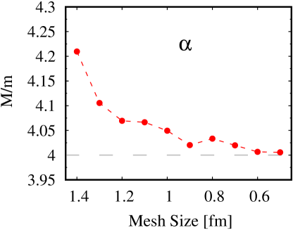
Using Eq. (11) we calculate the translational inertia mass of one alpha particle. The right panel of Fig. 1 shows the result as a function of mesh size. As the mesh size decreases, the results approach to the value of 4 in the unit of nucleon mass, which is the exact total mass of the alpha particle. With the simple BKN energy density functional, this exact value for the translation is also obtained with the cranking mass formula of Inglis. However, it underestimates the exact total mass when the energy functional has a effective mass . On the other hand, the ASCC mass for the translational motion is invariant and exact even with the effective mass. This is due to the Galilean symmetry of the energy density functional which inevitably contains the time-odd components. This will be discussed in Sec. III.4.
III.2 ASCC reaction path for +8Be
The numerical application of the ASCC method to determine a collective path for the nuclear fusion or fission reactions demands a substantial computational cost. Here, we present the result for the reaction path of +8Be, as the simplest example. It can be regarded as either the fusion path of two alpha particles or the fission path of 8Be. The model space is the three-dimensional grid space of the rectangular box of size fm3 with mesh size equal to 1.0 fm. The standard BKN energy density functional is adopted.
Starting from the two ground states of paticle and carrying out the iterative procedure presented in Sec. II.2, we obtain a fusion path that connects the two well separated alpha particles to the ground state of 8Be. If we start the calculation from the ground state of 8Be, the same reaction path, that represents fission of 8Be, can be obtained. In the left four panels of Fig. 2, we show the calculated density distribution of four different points on the obtained collective fusion path. The panel (a) shows the density distribution of two alpha particles at fm, (d) shows that of the ground state of 8Be which corresponds to fm. Those of (b) and (c) show those at fm and fm, respectively. The collective path smoothly evolves the separated two alpha particles into the ground state of 8Be.
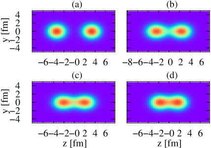
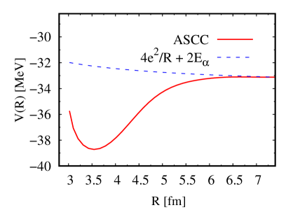
The right panel of Fig. 2 shows the potential energy along this collective path, as a function of . The dashed cure shows the point Coulomb potential, , with the ground state energy of a single alpha particle . With the BKN energy density functional, the 8Be is bound in the mean-field level. The ground state of 8Be is located in the potential minimum at fm, while the Coulomb barrier top is at fm. This ASCC collective path is self-consistently generated by the iterative procedure presented in Sec. II.2. The generators for the relative motion are microscopically given. Since the structure of the 8Be nucleus is very simple, this potential surface is actually similar to that of the constraint Hartree-Fock calculation.
III.3 Inertial mass for +8Be
Upon the collective reaction path obtained, the inertial mass with respect to the relative distance , , is calculated using Eq. (11). In the asymptotic region, we expect the inertial mass to be identical to the reduced mass, , where is the nucleon mass. For the current system +8Be, the value of is expected to be .
The reduced mass is justifiable when two alpha particles are well separated. However, it loses its validity as two particles approach each other. A widely used approach to calculate inertial mass for nuclear collective motion is the “Constrained-Hartree-Fock-plus-cranking” (CHF+cranking) approach (Baran et al., 2011). In this approach, the collective path is produced by the CHF calculation with a constraining operator given by hand, and the inertial mass is calculated based on the cranking formula with respect to these CHF states. The formula for the cranking mass can be derived by the adiabatic perturbation (Ring and Schuck, 1980). In the present case of the one-dimensional motion, based on the states constructed by the CHF calculation with a given constraining operator , the cranking formula reads (Baran et al., 2011)
| (14) |
where the single-particle states and their energies are defined with respect to ,
| (15) |
We may use any operator as a constraint, as far as it can generate the states with all the necessary values of . However, obviously the inertial mass depends on this choice, which is one of drawbacks of the CHF+cranking approach.
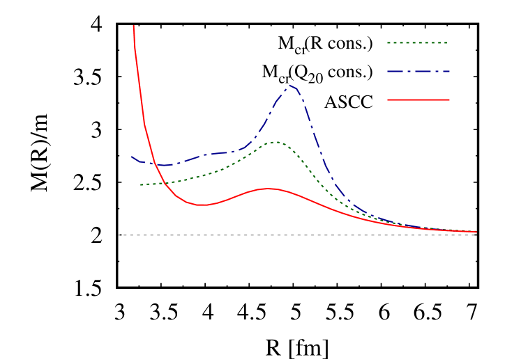
In most of the reaction models, the inertial mass with respect to is assumed to be a constant value of . Our study reveales how the inertia changes as a function of . In Fig. 3, both the ASCC and the cranking masses are presented. For the cranking mass, since the CHF state needs to be prepared first. We calculate the CHF states in two ways with different constraining operators ; the mass quadrupole operator and the relative distance operator of Eq. (10). The model space for both calculations are the same. As we can see from figure 3, at large distance, both methods asymptotically reproduce the reduced mass of , which is the exact value for the relative motion between two alpha particles. In the interior region where the two nuclei have merged into one system, these three masses give very different values. Generally the cranking mass is found to be larger than the ASCC mass, especially at around fm where all the three masses develop a bump structure.
The difference between the ASCC and the cranking masses attributes to several factors. One is due to the fact that the cranking formula neglects residual fields induced by the density fluctuation. Another is that the constraining operators affect the single-particle energies . We also note that the cranking masses obtained with different constraints give very different values. This is true even at the HF ground state ( fm), in which the single-particle states and their single-particle energies are all identical to each other. This is because the derivative gives different values, since the different constraint produces different states away from the HF ground state. This ambiguity exposes another drawback of the CHF+cranking approach, while the ASCC mass has an advantage that the collective coordinate as well as the wave functions are self-consistently calculated rather than artificially assumed.
III.4 Impact of time-odd potential
All the results shown so far are obtained with the standard BKN energy density functional that has no derivative terms. Therefore, the nucleon’s effective mass is identical to the bare nucleon mass. However, most of realistic effective interactions have effective mass smaller than the bare mass, typically . In such cases, an improper treatment of the collective dynamics leads to a wrong answer for the collective inertial mass (Thouless and Valatin, 1962). This change in the effective mass typically comes from the term in the Skyrme energy density functional, which should accompany the term to restore the Galilean symmetry (Thouless and Valatin, 1962; Bohr and Mottelson, 1975). These terms are absent in the standard BKN functional.
To investigate the effect of the time-odd mean-field potential on the collective inertial mass, we add the term to the original BKN energy density functional. The modified BKN energy density functional reads,
| (16) | |||||
where , , and are the isoscalar density, the isoscalar kinetic density, and the isoscalar current density, respectively. In equation (16), is the sum of the Yukawa and the Coulomb potentials (Bonche et al., 1976). The variation of the total energy with respect to the density (or equivalently single-particle wave functions) defines the single-particle (Hartree-Fock) Hamiltonian. In the present case, the single-particle Hamiltonian turns out to be
| (17) | |||||
where the effective mass is now deviated from bare nucleon mass
| (18) |
For the time-even states, such as the ground state of even-even nuclei, the current density disappears, . Even though, these terms play an important role in the collective inertial mass. The parameter provides the effective mass and the time-odd effect. The rest of the parameters are the same as those in reference (Bonche et al., 1976).
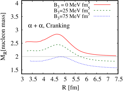
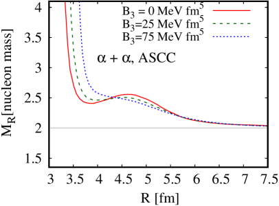
To examine the impact of the time-odd terms on the inertial mass, in Fig. (4) we show calculated with and without the term. When the time-odd terms are absent, , both the ASCC and the cranking formula reproduce the reduced mass in the asymptotic limit (). However, the cranking formula fails to do so with . As the value of increases, the asymptotic cranking mass decreases. This can be naively expected from the reduction of the effective mass from the bare mass. In contrast, the ASCC inertial mass converges to the correct reduced mass, no matter what values are. This means that the ASCC method is capable of taking into account the time-odd effect and recovering the exact Galilean symmetry.
Another inertial mass indispensable in the collective Hamiltonian of nuclear reaction models is the rotational moments of inertia. The rotational motion is a Nambu-Goldstone (NG) mode. To calculate this, we utilize a method proposed in the reference (Hinohara, 2015), where the inertial masses of the NG modes are calculated from the zero-frequency linear response with the momentum operator of the NG modes. The formulation has been tested in the cases of translational and pairing rotational modes, showing high precision and efficiency. Based on the collective path obtained, we apply this technique to calculate the rotational moments of inertia.
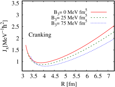
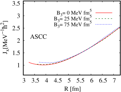
In figure 5, the calculated moments of inertias are presented. With , the moments of inertia calculated with the ASCC and with the cranking formula well agree with each other in the asymptotic region of large . The value is equal to the point-mass approximation in which the point particles are assumed at the center of mass of each particle. However, when non-zero comes in, the cranking mass formula can no longer reproduce this asymptotic value. Similar to the case of relative motion, as the value of increases, the asymptotic moments of inertia decrease and deviate from the asymptotic value. In contrast, the ASCC method provides the moments of inertia almost invariant with respect to the values. These results show again that, compared with the cranking formula, the ASCC method gives the collective inertial masses by properly taking into account the time-odd effects.
IV Summary and discussion
Based on the ASCC theory, we presented a method to determine the collective reaction path for the nuclear reaction as the large amplitude collective motion. This method is applied to the fusion/fission +8Be, using the BKN energy density functional. In the three-dimensional coordinate-space representation, the reaction path, the collective potential, as well as the inertial masses are self-consistently calculated. We compare the ASCC results with those of the CHF+cranking method. Since the reaction system is very simple, there is no significant difference between the calculated CHF reaction paths with different constraint operators. Despite of this similarity in the CHF states, the inertial masses calculated with the cranking formula turn out to sensitively depend on the choice of the constraint operator. The ASCC method is able to remove this ambiguity in the inertial mass, by taking into account the residual effects caused by the density fluctuation.
We add a term, which introduce the effective mass and time-odd mean fields, to the standard BKN energy density functional, to examine the effect of these terms on the inertial masses for both the relative and rotational motions. In the presence of time-odd term, the cranking formula fails to preserve the correct asymptotic values, while the validity of ASCC mass is not affected by the introduction of the effective mass. The time-odd mean-fields properly recover the Galilean symmetry, leading to the exact values of the asymptotic inertial mass. This is found to be true in both relative and rotational motions. With this property, we are quite confident that the ASCC method is promising to be applied to the modern nuclear energy density functionals, and make advanced microscopic theoretical analysis on various nuclear reaction models. Another important issue is the inclusion of the paring correlation, which may influence not only static but also dynamical nuclear properties. In order to keep the lowest-energy configuration during the collective motion, the pairing interaction is known to play a key role (Nakatsukasa et al., 2016b). Therefore, we may expect significant impact on both the collective inertial masses and the reaction paths. To study the above issues are our future tasks.
Acknowledgments
This work is supported in part by JSPS KAKENHI Grant No. 19H05142 and No. 18H01209, and also by JSPS-NSFC Bilateral Program for Joint Research Project on Nuclear mass and life for unravelling mysteries of r-process. This research in part used computational resources provided through the HPCI Sysytem Research Project (Project ID: hp190031) and by Multidisciplinary Cooperative Research Program in Center for Computational Sciences, University of Tsukuba.
Acknowledgements.
This work is supported in part by JSPS KAKENHI Grant No. 19H05142, and also by JSPS-NSFC Bilateral Program for Joint Research Project on Nuclear mass and life for unravelling mysteries of r- process. This research in part used computational resources provided through the HPCI Sysytem Research Project (Project ID: hp190031) and by Multidisciplinary Cooperative Research Program in Center for Computational Sciences, University of Tsukuba. This work is supported in part by JSPS KAKENHI Grants No. 25287065 and by Interdisciplinary Computational Science Program in CCS, University of Tsukuba.References
- Negele (1982) J. W. Negele, Rev. Mod. Phys. 54, 913 (1982).
- Simenel (2012) C. Simenel, The European Physical Journal A 48, 1 (2012).
- Nakatsukasa (2012) T. Nakatsukasa, Prog. Theor. Exp. Phys. 2012 (2012), 10.1093/ptep/pts016, 01A207.
- Maruhn et al. (2014) J. A. Maruhn, P.-G. Reinhard, P. D. Stevenson, and A. S. Umar, Computer Physics Communications 185, 2195 (2014).
- Nakatsukasa et al. (2016a) T. Nakatsukasa, K. Matsuyanagi, M. Matsuo, and K. Yabana, Rev. Mod. Phys. 88, 045004 (2016a).
- Ring and Schuck (1980) P. Ring and P. Schuck, The Nuclear Many-Body Problem (Springer-Verlag, New York, 1980).
- Blaizot and Ripka (1986) J. P. Blaizot and G. Ripka, Quantum theory of finite systems (MIT Press, Cambridge, 1986).
- Baranger and Kumar (1968a) M. Baranger and K. Kumar, Nuclear Physics A 110, 490 (1968a).
- Baranger and Kumar (1968b) M. Baranger and K. Kumar, Nuclear Physics A 122, 241 (1968b).
- Yuldashbaeva et al. (1999) E. Yuldashbaeva, J. Libert, P. Quentin, and M. Girod, Physics Letters B 461, 1 (1999).
- Marumori et al. (1980) T. Marumori, T. Maskawa, F. Sakata, and A. Kuriyama, Prog. Theor. Phys. 64, 1294 (1980).
- Matsuo et al. (2000) M. Matsuo, T. Nakatsukasa, and K. Matsuyanagi, Prog. Theor. Phys. 103 (5), 959 (2000).
- Hinohara et al. (2007) N. Hinohara, T. Nakatsukasa, M. Matsuo, and K. Matsuyanagi, Prog. Theor. Phys. 117 (3), 451 (2007).
- Hinohara et al. (2009) N. Hinohara, T. Nakatsukasa, M. Matsuo, and K. Matsuyanagi, Phys. Rev. C 80, 014305 (2009).
- Hinohara et al. (2012) N. Hinohara, Z. P. Li, T. Nakatsukasa, T. Nikšić, and D. Vretenar, Phys. Rev. C 85, 024323 (2012).
- Sato et al. (2012) K. Sato, N. Hinohara, K. Yoshida, T. Nakatsukasa, M. Matsuo, and K. Matsuyanagi, Phys. Rev. C 86, 024316 (2012).
- Davies et al. (1980) K. Davies, H. Flocard, S. Krieger, and M. Weiss, Nuclear Physics A 342, 111 (1980).
- Nakatsukasa et al. (2007) T. Nakatsukasa, T. Inakura, and K. Yabana, Phys. Rev. C 76, 024318 (2007).
- Inakura et al. (2009) T. Inakura, T. Nakatsukasa, and K. Yabana, Phys. Rev. C 80, 044301 (2009).
- Avogadro and Nakatsukasa (2011) P. Avogadro and T. Nakatsukasa, Phys. Rev. C 84, 014314 (2011).
- Avogadro and Nakatsukasa (2013) P. Avogadro and T. Nakatsukasa, Phys. Rev. C 87, 014331 (2013).
- Wen and Nakatsukasa (2016) K. Wen and T. Nakatsukasa, Phys. Rev. C 94, 054618 (2016).
- Egido et al. (2016) J. L. Egido, M. Borrajo, and T. R. Rodríguez, Phys. Rev. Lett. 116, 052502 (2016).
- Li et al. (2012) Z. P. Li, T. Nikšić, P. Ring, D. Vretenar, J. M. Yao, and J. Meng, Phys. Rev. C 86, 034334 (2012).
- Bonche et al. (1976) P. Bonche, S. Koonin, and J. W. Negele, Phys. Rev. C 13, 1226 (1976).
- Baran et al. (2011) A. Baran, J. A. Sheikh, J. Dobaczewski, W. Nazarewicz, and A. Staszczak, Phys. Rev. C 84, 054321 (2011).
- Thouless and Valatin (1962) D. J. Thouless and J. G. Valatin, Nucl. Phys. 31, 211 (1962).
- Bohr and Mottelson (1975) A. Bohr and B. R. Mottelson, Nuclear Structure, Vol. II (W. A. Benjamin, New York, 1975).
- Hinohara (2015) N. Hinohara, Phys. Rev. C 92, 034321 (2015).
- Nakatsukasa et al. (2016b) T. Nakatsukasa, K. Matsuyanagi, M. Matsuzaki, and Y. R. Shimizu, Physica Scripta 91, 073008 (2016b).