Zeroth-Order Algorithms for Nonconvex-Strongly-Concave Minimax Problems with Improved Complexities

Abstract

In this paper, we study zeroth-order algorithms for minimax optimization problems that are nonconvex in one variable and strongly-concave in the other variable. Such minimax optimization problems have attracted significant attention lately due to their applications in modern machine learning tasks. We first consider a deterministic version of the problem. We design and analyze the Zeroth-Order Gradient Descent Ascent (ZO-GDA) algorithm, and provide improved results compared to existing works, in terms of oracle complexity. We also propose the Zeroth-Order Gradient Descent Multi-Step Ascent (ZO-GDMSA) algorithm that significantly improves the oracle complexity of ZO-GDA. We then consider stochastic versions of ZO-GDA and ZO-GDMSA, to handle stochastic nonconvex minimax problems. For this case, we provide oracle complexity results under two assumptions on the stochastic gradient: (i) the uniformly bounded variance assumption, which is common in traditional stochastic optimization, and (ii) the Strong Growth Condition (SGC), which has been known to be satisfied by modern over-parametrized machine learning models. We establish that under the SGC assumption, the complexities of the stochastic algorithms match that of deterministic algorithms. Numerical experiments are presented to support our theoretical results.

1 Introduction

Algorithms for solving optimization problems with only access to (noisy) evaluations of the objective function are called zeroth-order algorithms. These algorithms have been studied for decades in the optimization literature; see, for example, [13, 50, 3] for a detailed overview of the existing approaches. Recently, the study of zeroth-order optimization algorithms has gained significant attention also in the machine learning literature, due to several motivating applications, for example, in designing black-box attacks to deep neural networks [14], hyperparameter tuning [53], reinforcement learning [34, 52] and bandit convex optimization [8]. However, a majority of the zeroth-order optimization algorithms in the literature has been developed for minimization problems.

In this work, we study zeroth-order optimization algorithms for solving nonconvex minimax problems (aka saddle-point problems). Specifically, we consider both the deterministic setting:

$$\min_{x\in\mathbb{R}^{d_{1}}}\max_{y\in\mathcal{Y}}f(x,y),$$ (1)

and the stochastic setting:

$$\min_{x\in\mathbb{R}^{d_{1}}}\max_{y\in\mathcal{Y}}f(x,y)=\textsf{\text{E}}_{\xi\sim\mathcal{P}}F(x,y,\xi).$$ (2)

Here, $F(x,y,\xi)$ and hence $f(x,y)$ are assumed to be sufficiently smooth functions, $\mathcal{Y}\subset\mathbb{R}^{d_{2}}$ is a closed and convex constraint set, and $\mathcal{P}$ is a distribution characterizing the stochasticity in the problem. We allow for the function $f(\cdot,y)$ to be nonconvex for all $y\in\mathbb{R}^{d_{2}}$ but require $f(x,\cdot)$ to be strongly-concave for all $x\in\mathbb{R}^{d_{1}}$. One of our main motivations for studying zeroth-order algorithms for nonconvex minimax problems is their application in designing black-box attacks to deep neural networks. By now, it is well established that care must be taken when designing and training deep neural networks as it is possible to design adversarial examples that would make the deep network to misclassify, easily. Since the intriguing works of [55, 26], the problem of designing such adversarial examples that transfer across multiple deep neural networks models has also been studied extensively. As the model architecture is unknown to the adversary, the problem could naturally be formulated to solve a minimax optimization problem under the availability of only (noisy) objective function evaluation. We refer the reader to [28] for details regarding such formulations. Apart from the above applications, we also note that zeroth-order minimax optimization problems also arise in multi-agent reinforcement learning with bandit feedback [60, 67], robotics [61, 11] and distributionally robust optimization [37].

Recently, there has been an ever-growing interest in analyzing first-order algorithms for the case of nonconvex-concave and nonconvex-nonconcave minimax problems, motivated by its applications to training generative adversarial networks [22], AUC maximization [65], designing fair classifiers [1], robust learning systems [32] fair machine learning [66, 63, 10], and reinforcement learning [46, 18, 42, 19]. Specifically, [29, 49, 41, 51, 27, 56] proposed and analyzed variants of gradient descent ascent for nonconvex-concave objectives. Very recently, under a stronger mean-squared Lipschitz gradient assumption [30] obtained improved complexities for stochastic nonconvex-concave objectives. Furthermore, [16, 17, 24, 33, 45, 20, 43, 25, 58] studied general nonconvex-nonconcave objectives.

Compared to first-order algorithms, zeroth-order algorithms for minimax optimization problems are underdeveloped. Motivated by the need for robustness in optimization, [36] proposed derivative-free algorithms for saddle-point optimization. However, they do not provide non-asymptotic oracle complexity analysis. Bayesian optimization algorithms and evolutionary algorithms were proposed in [11, 44] and [9, 2] respectively for minimax optimization, targeting robust optimization and learning applications. The above works do not provide any oracle complexity analysis. Recently, [48] studied zeroth-order Frank-Wolfe algorithms for strongly-convex and strongly-concave constrained saddle-point optimization problems and provided non-asymptotic oracle complexity analysis. Furthermore, [28] studied zeroth-order algorithms for nonconvex-concave minimax problems, similar to our setting. More recently, [4] proposed a stochastic direct search method for (2) under the assumption of the Polyak-Łojasiewicz (PL) condition. [64] and [23] also studied zeorth-order methods for (2), where they required mean-squared smoothnesss assumption, which is stronger than our assumptions.

Our Contributions. In this work, we consider both deterministic and stochastic minimax problems in the form of (1) and (2), respectively. A detailed comparison of our algorithms and existing methods is given in Table 1. Our contributions lie in several folds.

1. For deterministic minimax problem (1), we design a zeroth-order gradient descent ascent (ZO-GDA) algorithm, whose oracle complexity improves the currently best known one in [28] under the same assumptions. Notably, for this algorithm, the set $\mathcal{Y}$ could be constrained or unconstrained (i.e., the entire Euclidean space $\mathbb{R}^{d_{2}}$).

2. For deterministic minimax problem (1), we propose a novel zeroth-order gradient descent multi-step ascent (ZO-GDMSA) algorithm, which is motivated by [41]. This algorithm performs multiple steps of gradient ascent followed by one single step of gradient descent in each iteration. Its oracle complexity is significantly better than that of ZO-GDA in terms of the condition number dependency. To the best of our knowledge, this is the best complexity result for zeroth-order algorithms for solving deterministic minimax problems so far under the assumptions in Section 2.

3. We desgin and analyze the stochastic counterparts of ZO-GDA and ZO-GDMSA and establish their oracle complexity under two settings: (i) uniformly bounded variance assumption on the stochastic gradient, which is standard in stochastic optimization, and (ii) the Strong Growth Condition (SGC) [57], which is satisfied by modern overparametrized machine learning models. Notably, under SGC, we show that the complexities of the stochastic algorithms are the same as their deterministic counterparts.

Algorithm	Order	Complexity	Objective function	Constraint $(x,y)$
GDmax ([27])	1st	$\mathcal{O}(\kappa^{2}\epsilon^{-2})$	NC-SC	U,C
SGDmax ([27])	1st	$\mathcal{O}(\kappa^{3}(\sigma_{1}^{2}+\sigma_{2}^{2})\epsilon^{-4})$	NC-SC	U,C
Multi-step GDA([41])	1st	$\tilde{\mathcal{O}}(\log(\epsilon^{-1})\epsilon^{-2})$	NC-PL	C,U
Multi-step GDA ([41])	1st	$\tilde{\mathcal{O}}(\log(\epsilon^{-1})\epsilon^{-3.5})$	NC-C	C,C
ZO-min-max([28])	0th	$\tilde{\mathcal{O}}((d_{1}+d_{2})\epsilon^{-6})$	NC-SC	C,C
ZO-GDA	0th	$\mathcal{O}(\kappa^{5}(d_{1}+d_{2})\epsilon^{-2})$	NC-SC	U,C or U
ZO-GDMSA	0th	$\mathcal{O}(\kappa(d_{1}+\kappa d_{2}\log(\epsilon^{-1}))\epsilon^{-2})$	NC-SC	U,C
ZO-SGDA (Assmp. 2)	0th	$\mathcal{O}(\kappa^{5}(\sigma_{1}^{2}d_{1}+\sigma_{2}^{2}d_{2})\epsilon^{-4})$	NC-SC	U,C or U
ZO-SGDMSA (Assmp. 2)	0th	$\mathcal{O}(\kappa(d_{1}\sigma_{1}^{2}+\kappa d_{2}\sigma_{2}^{2}\log(\epsilon^{-1}))\epsilon^{-4})$	NC-SC	U,C
ZO-SGDA (Assmp. 3)	0th	$\mathcal{O}(\kappa^{5}(\rho_{1}d_{1}+\rho_{2}d_{2})\epsilon^{-2})$	NC-SC	U,C or U
ZO-SGDMSA (Assmp. 3)	0th	$\mathcal{O}(\kappa(d_{1}\rho_{1}+\kappa d_{2}\rho_{2}\log(\epsilon^{-1}))\epsilon^{-2})$	NC-SC	U,C

Table 1: Comparison of different algorithms. The column of “Complexity” gives the complexity of calls to zeroth-order oracle or first-order oracle. Here, we use $\tilde{\mathcal{O}}$ to hide the $\kappa$ dependency (where $\kappa$ refers to the condition number as defined in Assumption 1), as it was not explictly tracked and stated in [28, 41]. In the column of “Objective function” column, “NC-SC” indicates that the objective function is nonconvex with respect to $x$ and strongly concave with respect to $y$. “C” indicates that the function is concave with respect to $y$. PL denotes the Polyak-Łojasiewicz condition. In the column of “Constraint”, “C” means “constrained” and “U” means “unconstrained”.

The rest of this paper is organized as follows. In Section 2 we provide some preliminaries and introduce our zeroth-order gradient estimator. In Section 3 we present our ZO-GDA and ZO-GDMSA for solving the deterministic minimax problem (1), and analyze their oracle complexities. In Section 4 we present the stochastic algorithms ZO-SGDA and ZO-SGDMSA for solving the stochastic minimax problem (2), and analyze their oracle complexities. In Section 5 we provide some numerical results to our stochastic algorithms ZO-SGDA and ZO-SGDMSA for solving a distributionally robust optimization problem. We draw some conclusions in Section 6. Proofs of all theorems are provided in the appendix.

2 Preliminaries

Assumption 1 is made throughout the paper.

Assumption 1

The objective function $f(x,y)$ and the constraint set $\mathcal{Y}$ have the following properties:

• $f(x,y)$ is continuously differentiable in $x$ and $y$, and $f(\cdot,y)$ could be potentially nonconvex for all $y\in\mathcal{Y}$ and $f(x,\cdot)$ is $\tau$-strongly concave for all $x\in\mathbb{R}^{d_{1}}$.

• When viewed as a function in $\mathbb{R}^{d_{1}+d_{2}}$, $f(x,y)$ is $\ell$-gradient Lipschitz. That is, there exists constant $\ell>0$ such that $\forall x_{1},x_{2}\in\mathbb{R}^{d_{1}},y_{1},y_{2}\in\mathcal{Y}.$

  $$\|\nabla f(x_{1},y_{1})-\nabla f(x_{2},y_{2})\|_{2}\leq\ell\|(x_{1},y_{1})-(x_{2},y_{2})\|_{2},$$ (3)

  We use $\kappa:=\ell/\tau$ to denote the problem condition number throughout this paper.

• The function $g(x):=\max_{y\in\mathcal{Y}}f(x,y)$ is lower bounded. Moreover, we assume that function $g$ is $L_{g}$-smooth, i.e., $\|\nabla g(x)-\nabla g(y)\|\leq L_{g}\|x-y\|_{2}$, for all $x,y\in\mathbb{R}^{d_{1}}$. As will be shown later in Lemma A.3, this is indeed true with $L_{g}=(1+\kappa)\ell$.

• The constraint set $\mathcal{Y}\subset\mathbb{R}^{d_{2}}$ is bounded and convex, with diameter $D>0$. The boundedness assumption can be relaxed (see Remark 9).

The following assumption, which is standard in the literature [40, 21, 7], will also be used in our paper.

Assumption 2 (Uniformly Bounded Variance)

For any $x\in\mathbb{R}^{d_{1}}$ and $y\in\mathcal{Y}$, the stochastic zeroth-order oracle outputs an estimator $F\left(x,y,\xi\right)$ of $f\left(x,y\right)$ such that $\textsf{\text{E}}_{\xi}[F\left(x,y,\xi\right)]=f\left(x,y\right)$ and $\textsf{\text{E}}_{\xi}[\nabla_{x}F\left(x,y,\xi\right)]=\nabla_{x}f\left(x,y\right)$, $\textsf{\text{E}}_{\xi}[\nabla_{y}F\left(x,y,\xi\right)]=\nabla_{y}f\left(x,y\right)$, $\textsf{\text{E}}_{\xi}(\|\nabla_{x}F(x,y,\xi)-\nabla_{x}f(x,y)\|_{2}^{2})\leq\sigma_{1}^{2}$, and $\textsf{\text{E}}_{\xi}(\|\nabla_{y}F(x,y,\xi)-\nabla_{y}f(x,y)\|_{2}^{2})\leq\sigma_{2}^{2}$.

In addition to Assumptions 1 and 2, motivated by over-parametrized models arising in modern machine learning problems [57], we also consider the following SGC assumption on the stochastic gradient.

Assumption 3 (Strong Growth Condition [57])

There exist $\rho_{1},\rho_{2}>1$ such that the following is true for the stochastic gradients:

$$\textsf{\text{E}}_{\xi}(\|\nabla_{x}F(x,y,\xi)\|_{2}^{2})\leq\rho_{1}\|\nabla_{x}f(x,y)\|_{2}^{2},\mbox{ and }\textsf{\text{E}}_{\xi}(\|\nabla_{y}F(x,y,\xi)\|_{2}^{2})\leq\rho_{2}\|\nabla_{y}f(x,y)\|_{2}^{2}.$$

This condition is widely observed to be satisfied in modern over-parametrized models (e.g., deep neural networks) and has been used extensively for minimization problems recently [31, 5, 35, 59, 47].

2.1 Zeroth-order gradient estimator

We now discuss the idea of zeroth-order gradient estimator based on Gaussian smoothing technique [40]. For the deterministic case, we denote $\boldsymbol{u}_{1}\sim N(0,\textbf{1}_{d_{1}})$, $\boldsymbol{u}_{2}\sim N(0,\textbf{1}_{d_{2}})$, where $\textbf{1}_{d_{1}}$ and $\textbf{1}_{d_{2}}$ denote identity matrices with sizes $d_{1}\times d_{1}$ and $d_{2}\times d_{2}$, respectively. The notion of the Gaussian smoothed functions is defined as follows:

$$f_{\mu_{1}}(x,y): =\textsf{\text{E}}_{\boldsymbol{u}_{1}}f(x+\mu_{1}\boldsymbol{u}_{1},y),$$ (4)

$$f_{\mu_{2}}(x,y): =\textsf{\text{E}}_{\boldsymbol{u}_{2}}f(x,y+\mu_{2}\boldsymbol{u}_{2}),$$

and the zeroth-order gradient estimators [40] are defined as

$$G_{\mu_{1}}(x,y,\boldsymbol{u}_{1}) =\frac{f(x+\mu_{1}\boldsymbol{u}_{1},y)-f(x,y)}{\mu_{1}}\boldsymbol{u}_{1},$$ (5)

$$H_{\mu_{2}}(x,y,\boldsymbol{u}_{2}) =\frac{f(x,y+\mu_{2}\boldsymbol{u}_{2})-f(x,y)}{\mu_{2}}\boldsymbol{u}_{2},$$

where $\mu_{1}>0$ and $\mu_{2}>0$ are smoothing parameters.

As noted in [6], the Gaussian smoothing technique proposed by [40] is based on the Stein’s identity [54], for characterizing Gaussian random vectors. Specifically, Stein’s identity states that a random vector $u\in\mathbb{R}^{d}$, is standard Gaussian if and only if, $\textsf{\text{E}}\left[u~{}h(u)\right]=\textsf{\text{E}}\left[\nabla h(u)\right]$, for all absolutely continuous functions $h:\mathbb{R}^{d}\to\mathbb{R}$. Note that Stein’s identity, naturally relates function queries to gradients and thus is naturally suited for zeroth-order optimization. If we let $h(u)$ to be the Gaussian smoothed functions (as in (4)), it is easy to see that the zeroth-order gradients (as in (5)) follow by simply evaluating the Gaussian Stein’s identity.

It should be noted following the arguments in [40, 7] that $\textsf{\text{E}}_{\boldsymbol{u}_{1}}G_{\mu_{1}}(x,y,\boldsymbol{u}_{1})=\nabla_{x}f_{\mu_{1}}(x,y)$, and $\textsf{\text{E}}_{\boldsymbol{u}_{2}}G_{\mu_{2}}(x,y,\boldsymbol{u}_{2})=\nabla_{y}f_{\mu_{2}}(x,y)$. Hence, the zeroth-order gradient estimators in (5) provide unbiased estimates of the gradient of Gaussian smoothed functions $f_{\mu_{1}}(x,y,\boldsymbol{u}_{1}):=f(x+\mu_{1}\boldsymbol{u}_{1},y)$ and $f_{\mu_{2}}(x,y,\boldsymbol{u}_{2}):=f(x,y+\mu_{2}\boldsymbol{u}_{2})$. Similarly, for the stochastic case, the Gaussian smoothed functions are defined as:

$$f_{\mu_{1}}(x,y):=\textsf{\text{E}}_{\boldsymbol{u}_{1},\xi}F(x+\mu_{1}\boldsymbol{u}_{1},y,\xi),$$ (6)

$$f_{\mu_{2}}(x,y):=\textsf{\text{E}}_{\boldsymbol{u}_{2},\xi}F(x,y+\mu_{2}\boldsymbol{u}_{2},\xi),$$

and the zeroth-order stochastic gradient estimators are defined as:

$$G_{\mu_{1}}(x,y,\boldsymbol{u}_{1},\xi)=\frac{F(x+\mu_{1}\boldsymbol{u}_{1},y,\xi)-F(x,y,\xi)}{\mu_{1}}\boldsymbol{u}_{1},$$ (7)

$$H_{\mu_{2}}(x,y,\boldsymbol{u}_{2},\xi)=\frac{F(x,y+\mu_{2}\boldsymbol{u}_{2},\xi)-F(x,y,\xi)}{\mu_{2}}\boldsymbol{u}_{2}.$$

One can also show that the zeroth-order gradient estimators provide unbiased estimates to the gradients of the Gaussian smoothed functions, i.e., $\textsf{\text{E}}_{\boldsymbol{u}_{1},\xi}G_{\mu_{1}}(x,y,\boldsymbol{u}_{1},\xi)=\nabla_{x}f_{\mu_{1}}(x,y),$ and $\textsf{\text{E}}_{\boldsymbol{u}_{2},\xi}H_{\mu_{2}}(x,y,\boldsymbol{u}_{2},\xi)=\nabla_{y}f_{\mu_{2}}(x,y).$

In our algorithms, we also need to use mini-batch zeroth-order gradient estimators, which can reduce the variance of stochastic gradient estimators. To this end, we define the following notation. For integer $q>0$, we denote $[q]:=\{1,\ldots,q\}$. In the deterministic case, for integers $q_{1}>0$, $q_{2}>0$ we denote

$$G_{\mu_{1}}(x,y,\boldsymbol{u}_{1,[q_{1}]})=\frac{1}{q_{1}}\sum_{i=1}^{q_{1}}G_{\mu_{1}}(x,y,\boldsymbol{u}_{1,i}),$$ (8)

$$H_{\mu_{2}}(x,y,\boldsymbol{u}_{2,[q_{2}]})=\frac{1}{q_{2}}\sum_{i=1}^{q_{2}}H_{\mu_{2}}(x,y,\boldsymbol{u}_{2,i}).$$

For indices sets $\mathcal{M}_{1}$ and $\mathcal{M}_{2}$, in the stochastic case we denote

$$\begin{array}[]{ll}G_{\mu_{1}}(x,y,\boldsymbol{u}_{\mathcal{M}_{1}},\xi_{\mathcal{M}_{1}})&=\frac{1}{|\mathcal{M}_{1}|}\sum_{i\in\mathcal{M}_{1}}G_{\mu_{1}}(x,y,\boldsymbol{u}_{1,i},\xi_{i}),\\ H_{\mu_{2}}(x,y,\boldsymbol{u}_{\mathcal{M}_{2}},\xi_{\mathcal{M}_{2}})&=\frac{1}{|\mathcal{M}_{2}|}\sum_{i\in\mathcal{M}_{2}}H_{\mu_{2}}(x,y,\boldsymbol{u}_{2,i},\xi_{i}).\end{array}$$ (9)

It is easy to see that we have the following unbiasedness properties:

$$\textsf{\text{E}}_{\boldsymbol{u}_{1,[q_{1}]}}G_{\mu_{1}}(x,y,\boldsymbol{u}_{1,[q_{1}]})=\nabla_{x}f_{\mu_{1}}(x,y)\mbox{ and }\textsf{\text{E}}_{\boldsymbol{u}_{2,[q_{2}]}}H_{\mu_{2}}(x,y,\boldsymbol{u}_{2,[q_{2}]})=\nabla_{y}f_{\mu_{2}}(x,y)$$

and

$$\textsf{\text{E}}_{\boldsymbol{u}_{1}}\textsf{\text{E}}_{\xi_{\mathcal{M}_{1}}}G_{\mu_{1}}(x,y,\boldsymbol{u}_{\mathcal{M}_{1}},\xi_{\mathcal{M}_{1}})=\nabla_{x}f_{\mu_{1}}(x,y)$$

$$\textsf{\text{E}}_{\boldsymbol{u}_{2}}\textsf{\text{E}}_{\xi_{\mathcal{M}_{2}}}H_{\mu_{2}}(x,y,\boldsymbol{u}_{\mathcal{M}_{2}},\xi_{\mathcal{M}_{2}})=\nabla_{y}f_{\mu_{2}}(x,y).$$

2.2 Complexity Measure

Following [27], the $\epsilon$-stationary point of problems (1) and (2) and is defined as follows.

Definition 2.1

A point $(\bar{x},\bar{y})$ is called an $\epsilon$-stationary point of problem (1) and (2) if it satisfies the following conditions: $\textsf{\text{E}}(\|\nabla_{x}f(\bar{x},\bar{y})\|^{2}_{2})\leq\epsilon^{2}$ and $\textsf{\text{E}}(\|\nabla_{y}f(\bar{x},\bar{y})\|^{2}_{2})\leq\epsilon^{2}$. Here, the expectation is over $\textbf{u}_{1}$ and $\textbf{u}_{2}$ sequence for problem (1), and over the $\textbf{u}_{1}$, $\textbf{u}_{2}$ and $\xi$ sequence for problem (2). The $\textbf{u}_{1}$, $\textbf{u}_{2}$ and $\xi$ are randomness generated in the algorithm when $(\bar{x},\bar{y})$ is produced.

Note that the minimax problems (1) and (2) are equivalent to the following minimization problem:

$$\min_{x}\{g(x):=\max_{{y\in\mathcal{Y}}}f({x},{y})=f(x,y^{*}(x))\},$$ (10)

where $y^{*}(x)=\mathop{\rm argmax}_{y\in\mathcal{Y}}f(x,y)$. Due to our Assumption 1, that $f({x},\cdot)$ is strongly-concave for any fixed ${x}\in\mathbb{R}^{d_{1}}$, the maximization problem $\max_{y}f(x,y)$ can be solved efficiently and its optimal solution is unique. Note that the $\epsilon$-stationary point for (10) is defined as follows.

Definition 2.2

We call $\bar{x}$ an $\epsilon$-stationary point of a differentiable function $g$ if $\textsf{\text{E}}(\|\nabla g(\bar{x})\|^{2}_{2})\leq\epsilon^{2}$.

In this paper, we focus on analyzing the oracle complexity of algorithms for obtaining an $\epsilon$-stationary point of $g$ as defined in Definition 2.2. This is because optimality in the sense of Definition 2.2 in turn implies optimality in the sense of Definition 2.1, as we discuss in the following proposition.

Proposition 2.1

Under Assumption 1, if a point $\bar{x}$ satisfies $\textsf{\text{E}}(\|\nabla g(\bar{x})\|^{2}_{2})\leq\epsilon^{2}$, by using extra $\mathcal{O}(\kappa d_{2}\log(\epsilon^{-1}))$ calls to the zeroth order oracle in the deterministic setting or by using extra $\mathcal{O}(d_{2}/\epsilon^{2})$ calls to the zeroth order oracle in the stochastic setting, a point $(\bar{x},\bar{y})$ can be obtained such that it is an $\epsilon$-stationary solution of the minimax problem as defined in Definition 2.1.

The proof of this proposition is the same as the proof of Proposition 4.11 in [27]. We thus omit it for succinctness.

3 Zeroth-order Algorithms for Deterministic Minimax Problems

We now present our algorithms for the deterministic minimax problem (1).

3.1 Zeroth-Order Gradient Descent Ascent

Our zeroth-order gradient descent ascent (ZO-GDA) algorithm for solving problem (1) is described in Algorithm 1. The algorithm is similar to the deterministic first-order approach analyzed in [27] with some crucial differences. Specifically, we require a mini-batch gradient estimator with the choices of the batch size depending on the dimensionality of the problem.

Algorithm 1 Zeroth-Order Gradient Descent Ascent (ZO-GDA)

  Initialization: $(x_{0},y_{0})$, stepsizes $(\eta_{1},\eta_{2})$, iteration limit $S>0$, parameters $\mu_{1}$ and $\mu_{2}$. Set $q_{1}=2(d_{1}+6)$, $q_{2}=2(d_{2}+6)$.

  for $s=0,\ldots,S-1$ do

     $x_{s+1}\leftarrow x_{s}-\eta_{1}G_{\mu_{1}}(x_{s},y_{s},\boldsymbol{u}_{1,[q_{1}]})$ with $\boldsymbol{u}_{1,i}\sim N(0,\textbf{1}_{d_{1}})$, $i\in[q_{1}]$

     $y_{s+1}\leftarrow\text{Proj}_{\mathcal{Y}}[y_{s}+\eta_{2}H_{\mu_{2}}(x_{s},y_{s},\boldsymbol{u}_{2,[q_{2}]})]$ with $\boldsymbol{u}_{2,i}\sim N(0,\textbf{1}_{d_{2}})$, $i\in[q_{2}]$

  end for

  Return $(x_{1},y_{1}),\ldots,(x_{S},y_{S})$.

The complexity result for ZO-GDA (Algorithm 1) is provided in Theorem 1.

Theorem 1

Under Assumption 1, by setting

$$\eta_{1}:=\frac{1}{4\times 12^{4}\kappa^{2}(\kappa+1)^{2}(\ell+1)},~{}~{}\eta_{2}:=1/(6\ell),$$ (11)

and

$$S:=\mathcal{O}(\kappa^{5}\epsilon^{-2}),~{}~{}\mu_{1}:=\mathcal{O}(\epsilon d_{1}^{-3/2}\kappa^{-2}),~{}~{}\mu_{2}:=\mathcal{O}(\epsilon d_{2}^{-3/2}\kappa^{-2}),$$ (12)

ZO-GDA (Algorithm 1) returns iterates $(x_{1},y_{1}),\ldots,(x_{S},y_{S})$ such that there exists an iterate which is an $\epsilon$-stationary point of $g(x)=\max_{y\in\mathcal{Y}}f(x,y)$. That is, ZO-GDA (Algorithm 1) returns iterates that satisfy $\min_{s\in\{1,...,S\}}\textsf{\text{E}}(\|\nabla g(x_{s})\|_{2}^{2})\leq\epsilon^{2}$. Moreover, the total number of calls to the (deterministic) zeroth-order oracle is given by $K_{\mathcal{ZO}}=S(q_{1}+q_{2})=\mathcal{O}(\kappa^{5}(d_{1}+d_{2})\epsilon^{-2})$.

Remark 2

We see that the total number of calls to the (deterministic) zeroth-order oracle depends linearly on the dimension of the problem. The dependence on $\epsilon$ is the same as that of the corresponding first-order methods [27]. But, the dependence on the condition number $\kappa$ is increased from $\kappa^{2}$ to $\kappa^{5}$ (assuming $d_{1}$ and $d_{2}$ are of constant order). This is due to the choice of balancing the various tuning parameters in the zeroth-order setting, in particular $\mu_{1}$ and $\mu_{2}$ which are absent in the first-order setting.

3.2 Zeroth-Order Gradient Descent Multi-Step Ascent

We now present our ZO-GDMSA algorithm in Algorithm 2. This algorithm runs $T$ ascent steps, for every descent step. The main idea behind running multiple ascent steps is to better approximate the maximum of the stongly-concave function in each step. Subsequently, picking the number of inner iterations $T$ appropriately helps us obtain improved dependence on $\kappa$ while still maintaining the same dependency on $\epsilon$. We emphasize that [41] used the multi-step ascent approach to handle certain non-convex minimax optimization problems that satisfy the PL condition in the first-order setting.

Algorithm 2 Zeroth-Order Gradient Descent Multi-Step Ascent (ZO-GDMSA)

  Initialization: $\left(x_{0},y_{0}\right)$, step sizes $\left(\eta_{1},\eta_{2}\right)$, iteration limit for outer loop $S>0$, iteration limit for inner loop $T>0$, parameters $\mu_{1}$ and $\mu_{2}$. Set $q_{1}=2(d_{1}+6)$ and $q_{2}=2(d_{2}+6)$.

  for $s=0,\ldots,S-1$ do

     Set $y_{0}(x_{s})\leftarrow y_{s}$

     for $t=1,\ldots,T$ do

        $y_{t}(x_{s})\leftarrow\mathrm{Proj}_{\mathcal{Y}}(y_{t-1}(x_{s})+\eta_{2}H_{\mu_{2}}(x_{s},y_{t-1}(x_{s}),\boldsymbol{u}_{2,[q_{2}]}))$ with $\boldsymbol{u}_{2,i}\sim N(0,\textbf{1}_{d_{2}})$, $i\in[q_{2}]$

     end for

     $y_{s+1}\leftarrow y_{T}(x_{s})$

     $x_{s+1}\leftarrow x_{s}-\eta_{1}G_{\mu_{1}}(x_{s},y_{s+1},\boldsymbol{u}_{1,[q_{1}]})$ with $\boldsymbol{u}_{1,i}\sim N(0,\textbf{1}_{d_{1}})$, $i\in[q_{1}]$

  end for

  Return $(x_{1},y_{1}),\ldots,(x_{S},y_{S})$.

Theorem 3

Under Assumption 1, by setting

$${\eta_{1}=1/(12L_{g})=\frac{1}{12(1+\kappa)\ell}},\ \eta_{2}=1/(6\ell),\ T=\mathcal{O}(\kappa\log(\epsilon^{-1})),$$ (13)

and

$$S=\mathcal{O}(\kappa\epsilon^{-2}),\ \mu_{1}=\mathcal{O}({\epsilon}d_{1}^{-3/2}),\ \mu_{2}=\mathcal{O}(\kappa^{-1/2}d_{2}^{-3/2}\epsilon),$$ (14)

ZO-GDMSA (Algorithm 2) returns iterates $(x_{1},y_{1}),\ldots,(x_{S},y_{S})$ such that there exists an iterate which is an $\epsilon$-stationary point for $g(x)=\max_{y\in\mathcal{Y}}f(x,y)$. That is, ZO-GDMSA (Algorithm 2) returns iterates that satisfy $\min_{s\in\{1,...,S\}}\textsf{\text{E}}(\|\nabla g(x_{s})\|_{2}^{2})\leq\epsilon^{2}$. Moreover, the total number of calls to the (deterministic) zeroth-order oracle is given by $K_{\mathcal{ZO}}=Sq_{1}+TSq_{2}=\mathcal{O}\Bigl{(}\kappa\epsilon^{-2}(d_{1}+\kappa d_{2}\log(\epsilon^{-1}))\Bigr{)}.$

Remark 4

Compared to Algorithm 1, the oracle complexity of Algorithm 2 has improved dependence on $\kappa$ while maintaining the same dependence on $\epsilon$.

4 Zeroth-order Algorithms for Stochastic Minimax Problems

We now consider the stochastic minimax problem (2), under the availability of a stochastic zeroth-order oracle satisfying Assumption 2 or Assumption 3. This scenario is more practical in the context of zeroth-order optimization, as often times, we are able to only observe noisy evaluations of the function [13, 3]. Motivated by our analysis of the deterministic case, we now design and analyze the stochastic versions of ZO-GDA and ZO-GDMSA.

We first consider stochastic version of ZO-GDA, which is named ZO-SGDA and presented in Algorithm 3. Under Assumption 2, the main difference between Algorithm 3 and its deterministic counterpart (Algorithm 1) is in the choice of mini-batch size in the zeroth-order gradient estimator. As opposed to the deterministic case, where the mini-batch size is independent of $\epsilon$, in this case, we require a mini-batch size that depends on $\epsilon$. Furthermore, due to the stochastic nature of the problem, the mini-batch size also depends on the noise variance parameter $\sigma^{2}$. However, under Assumption 3, it suffices to have the batch size to be the same as in the deterministic case – this leads to the rate improvement. The complexity result corresponding to Algorithm 3 is provided in Theorem 5.

Algorithm 3 Zeroth-Order Stochastic Gradient Descent Ascent (ZO-SGDA)

  Initialization: $\left(x_{0},y_{0}\right)$, step sizes $\left(\eta_{1},\eta_{2}\right)$, iteration limit $S>0$, smoothing parameters $\mu_{1}$ and $\mu_{2}$. Indices sets $\mathcal{M}_{1}$ and $\mathcal{M}_{2}$.

  for $s=0,\ldots,S-1$ do

     $x_{s+1}\leftarrow x_{s}-\eta_{1}\frac{1}{|\mathcal{M}_{1}|}\sum_{i\in\mathcal{M}_{1}}G_{\mu_{1}}\left(x_{s},y_{s},\boldsymbol{u}_{1,i},\xi_{i}\right)$ with $\boldsymbol{u}_{1,i}\sim N(0,\textbf{1}_{d_{1}})$

     $y_{s+1}\leftarrow\text{Proj}_{\mathcal{Y}}\Bigl{[}y_{s}+\eta_{2}\frac{1}{|\mathcal{M}_{2}|}\sum_{i\in\mathcal{M}_{2}}H_{\mu_{2}}\left(x_{s},y_{s},\boldsymbol{u}_{2,i},\xi_{i}\right)\Bigr{]}$ with $\boldsymbol{u}_{2,i}\sim N(0,\textbf{1}_{d_{2}})$

  end for

  Return $(x_{1},y_{1}),\ldots,(x_{S},y_{S})$.

Theorem 5

Let $\epsilon\in(0,1)$. Then

1. Under Assumptions 1 and  2, by setting the parameters $\eta_{1},\eta_{2}$ as in (11), setting $S,\mu_{1},\mu_{2}$ as in (12), and setting $|\mathcal{M}_{1}|=4(d_{1}+6)(\sigma_{1}^{2}+1)\epsilon^{-2}$, $|\mathcal{M}_{2}|=4(d_{2}+6)(\sigma_{2}^{2}+1)\epsilon^{-2}$, ZO-SGDA (Algorithm 3) returns iterates $(x_{1},y_{1}),\ldots,(x_{S},y_{S})$ such that there exists an iterate which is an $\epsilon$-stationary point for $g(x)=\max_{y\in\mathcal{Y}}f(x,y)$. That is, ZO-SGDA (Algorithm 3) returns iterates that satisfy $\min_{s\in\{1,...,S\}}\textsf{\text{E}}(\|\nabla g(x_{s})\|_{2}^{2})\leq\epsilon^{2}$. Moreover, the total number of calls to the stochastic zeroth-order oracle is given by $K_{\mathcal{SZO}}=S(|\mathcal{M}_{1}|+|\mathcal{M}_{2}|)=\mathcal{O}(\kappa^{5}(d_{1}\sigma_{1}^{2}+d_{2}\sigma_{2}^{2})\epsilon^{-4})$.

2. Under Assumptions 1,  2 (only the unbiased part) and  3, by setting $|\mathcal{M}_{1}|=\rho_{1}(d_{1}+6)$, $|\mathcal{M}_{2}|=\rho_{2}(d_{2}+6)$ and setting $\mu_{1}=\mathcal{O}(\rho_{1}\ell d_{1}^{-3/2})$ and $\mu_{2}=\mathcal{O}(\rho_{2}\ell d_{2}^{-3/2})$, with other parameters remaining the same, the conclusion in Part 1 holds. In this case, the total number of calls to the stochastic zeroth-order oracle is given by $K_{\mathcal{SZO}}=S(|\mathcal{M}_{1}|+|\mathcal{M}_{2}|)=\mathcal{O}(\kappa^{5}(\rho_{1}d_{1}+\rho_{2}d_{2})\epsilon^{-2})$.

Remark 6

Under Assumption 2, the $\epsilon$-dependence of Algorithm 3 is the same as the first-order counterpart considered in [27]. However, under Assumption 3, the $\epsilon$-dependence is improved and is the same as the deterministic case.

The stochastic version of Algorithm 2 is named ZO-SGDMSA and presented in Algorithm 4. Its oracle complexity result is provided in Theorem 7.

Algorithm 4 Zeroth-Order Stochastic Gradient Multi-Step Descent (ZO-SGDMSA)

  Initialization: $\left(x_{0},y_{0}\right)$, step sizes $\left(\eta_{1},\eta_{2}\right)$, iteration limit for outer loop $S>0$, iteration limit for inner loop $T>0$, smoothing parameters $\mu_{1}$ and $\mu_{2}$. Indices sets $\mathcal{M}_{1}$ and $\mathcal{M}_{2}$.

  for $s=1,\ldots,S-1$ do

     Set $y_{0}(x_{s})\leftarrow y_{s}$

     for $t=1,\ldots,T$ do

        $y_{t}(x_{s})\leftarrow\text{Proj}_{\mathcal{Y}}\Bigl{[}y_{t-1}(x_{s})+\eta_{2}\frac{1}{|\mathcal{M}_{2}|}\sum_{i\in\mathcal{M}_{2}}H_{\mu_{2}}(x_{s},y_{t-1}(x_{s}),\boldsymbol{u}_{2,i},\xi_{i})\Bigr{]}$ with $\boldsymbol{u}_{2,i}\sim N(0,\textbf{1}_{d_{2}})$

     end for

     $y_{s+1}\leftarrow y_{T}(x_{s})$

     $x_{s+1}\leftarrow x_{s}-\eta_{1}\frac{1}{|\mathcal{M}_{1}|}\sum_{i\in\mathcal{M}_{1}}G_{\mu_{1}}(x_{s},y_{s+1},\boldsymbol{u}_{1,i},\xi_{i})$ with $\boldsymbol{u}_{1,i}\sim N(0,\textbf{1}_{d_{1}})$

  end for

  Return $(x_{1},y_{1}),\ldots,(x_{S},y_{S})$.

Theorem 7

Let $\epsilon\in(0,1)$. Then,

1. Under Assumptions 1 and  2, by setting $\eta_{1},\eta_{2}$ as in (13), $S,\mu_{1},\mu_{2}$ as in (14), and setting $|\mathcal{M}_{1}|=4(d_{1}+6)(\sigma_{1}^{2}+1)\epsilon^{-2}$, $|\mathcal{M}_{2}|=4(d_{2}+6)(\sigma_{2}^{2}+1)\epsilon^{-2}$, ZO-SGDMSA (Algorithm 4) returns iterates $(x_{1},y_{1}),\ldots,(x_{S},y_{S})$ such that there exists an iterate which is an $\epsilon$-stationary point for $g(x)=\max_{y\in\mathcal{Y}}f(x,y)$. That is, ZO-SGDMSA (Algorithm 4) returns iterates that satisfy $\min_{s\in\{1,...,S\}}\textsf{\text{E}}(\|\nabla g(x_{s})\|_{2}^{2})\leq\epsilon^{2}$. Moreover, the total number of calls to the stochastic zeroth-order oracle is given by, $K_{\mathcal{SZO}}=S|\mathcal{M}_{1}|+TS|\mathcal{M}_{2}|=\mathcal{O}(\kappa\epsilon^{-4}(d_{1}\sigma_{1}^{2}+\kappa d_{2}\sigma_{2}^{2}\log(\epsilon^{-1})))$.

2. Under Assumptions 1,  2 (only the unbiased part) and  3, by setting $|\mathcal{M}_{1}|=\rho_{1}(d_{1}+6)$, $|\mathcal{M}_{2}|=\rho_{2}(d_{2}+6)$ and setting $\mu_{1}=\mathcal{O}(\rho_{1}\ell d_{1}^{-3/2})$ and $\mu_{2}=\mathcal{O}(\rho_{2}\ell d_{2}^{-3/2})$, with other parameters remaining the same, the conclusion in Part 1 holds. In this case, the total number of calls to the stochastic zeroth-order oracle is given by, $K_{\mathcal{SZO}}=S|\mathcal{M}_{1}|+TS|\mathcal{M}_{2}|=\mathcal{O}(\kappa(\rho_{1}d_{1}+\kappa\rho_{2}d_{2}\log(\epsilon^{-1}))\epsilon^{-2})$.

Remark 8

Similar to the deterministic case, we improve the dependence of the oracle complexity on $\kappa$. The dependence on $\epsilon$ and dimensionality remains the same. We emphasize that the use of multiple steps in the ascent part, leads to the improved dependency on $\kappa$ over Algorithm 3.

5 Numerical Results

We now compare ZO-SGDA and ZO-SGDMSA with their first-order counterparts (i.e., SGDA and SGDMSA) on the distributionally robust optimization problem [37]. For simplicity, we present the formulation of the problem in the finite-sum setting as:

$$\min_{x\in\mathbb{R}^{d}}\max_{y\in\mathcal{Y}}\sum_{i=1}^{n}y_{i}\ell_{i}(x)-r(y),$$

where $\mathcal{Y}=\{y\in\mathbb{R}^{n}\mid\sum_{i=1}^{n}y_{i}=1,y_{i}\geq 0\}$ is the probability simplex; $r(y)=10\sum_{i=1}^{n}(y_{i}-1/n)^{2}$ is a divergence measure regularizing derivations from uniform distribution; $\ell_{i}(x)=f_{1}(f_{2}(x,s_{i},z_{i}))$ where $f_{1}(x)=\log(1+x)$, $f_{2}(x)=\log(1+\exp[-z_{i}(x^{T}s_{i})])$, $(s_{i},z_{i})$ is the feature and label pair of a sample $i$ in the dataset. It is easy to see that the above problem is a nonconvex-strongly concave minimax problem of the from (1) with $d_{1}=d,d_{2}=n$. For the tuning parameters, motivated by our theoretical results, we set the batch size $|\mathcal{M}_{1}|=d_{1}/\epsilon^{2}$ and $|\mathcal{M}_{2}|=d_{2}/\epsilon^{2}$ with $\epsilon=0.01$. For ZO-SGDA, we choose $\eta_{1}=\eta_{2}=0.01$, and for ZO-SGDMSA, we choose $\eta_{1}=0.001$ and $\eta_{2}=0.01$. For ZO-GDA and ZO-SGDA, according to Theroems 1 and 3, we chose

$$\mu_{1}=1.5\epsilon d_{1}^{-3/2}\kappa^{-2}\quad\mu_{2}=1.5\epsilon d_{2}^{-3/2}\kappa^{-2}.$$

For ZO-GDMSA and ZO-SGDMSA, according to Theorems 2 and 4, we chose

$$\mu_{1}=1.5\epsilon d_{1}^{-3/2}\quad\mu_{2}=1.5\kappa^{-1/2}d_{2}^{-3/2}\epsilon.$$

For our tested problems, we have $\kappa^{3}=10$ (see, for example [62]). The $\mu_{1}$ and $\mu_{2}$ in the above equations are usually at the order of $10^{-5}$ to $10^{-6}$. For SGDA and SGDMSA, we choose the same stepsize as ZO-SGDA and ZO-SGDMSA and set $|\mathcal{M}_{1}|=1/\epsilon^{2}$ and $|\mathcal{M}_{2}|=1/\epsilon^{2}$. We stop the iteration when $\|\nabla g(x_{s})\|_{2}\leq\epsilon$, based on our theoretical analysis. We test our algorithms on the following datasets from UCI ML-repository [15] and LIBSVM [12]: A9A , Mushroom ,W8A and Colon-cancer gene expression dataset. In order to perform distributionally robust optimization, we sample the dataset such that the positive and negative label ratio is 1:3. Details of these datasets are provided in Table 2. All the experiments were run on Google Colab Python 3.5 Notebook. We also remark that we cannot compare empirically to [28] as they consider constrained minimax problems. In Figure 1, we plot the value of the objective versus iteration number and the value of gradient size versus iteration number. We find that the proposed zeroth-order methods perform favorably to their respective first-order counterparts in terms of both the objective value and the norm of the gradient of the function $g$, as measured by iteration count. It should be noted that to obtain this comparable behavior, the zeroth-order method uses a mini-batch of samples that is proportional to the dimension (recall our choice of $|\mathcal{M}_{1}|$ and $|\mathcal{M}_{2}|$) above) in each iteration, which results in the number of calls to the zeroth-order oracle of the order as illustrated in our theoretical results.

Dataset	Samples	Features	T/F ratio
A9A	200	123	1:3
Mushroom	100	22	1:3
W8A	100	300	1:3
Colon-cancer	200	500	1:3

Table 2: Details of the datasets [15].

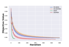
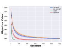
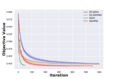
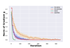
Figure 1: Performance of ZO-SGDA and ZO-SGDMSA in comparison to their first-order counterparts. The results in the four rows respectively correpond to the following datasets: A9A dataset, Mushroom dataset, W8A dataset and Colon Cancer dataset. The results correspond to average over 500 trails.

6 Conclusions

In this paper, we designed and analyzed zeroth-order algorithms for deterministic and stochastic nonconvex minimax problems. Specifically, we considered two types of algorithms: zeroth-order gradient descent ascent algorithm and a modified version of it with multiple ascent steps following each descent step. We obtained oracle complexities for both algorithms that match the performance of comparable first-order algorithms, up to unavoidable dimensionality factors. Our orcale complexities are better than that of existing methods under the same assumptions. Future works include to explore lower bounds for zeroth-order nonconvex minimax optimization problems, and to explore structural constraints to obtain improved dimensionality dependence in our results.

Appendix A Technical Preparations

In this section we present some technical results that will be used in our subsequent convergence analysis. First, we need the follow elementary results regarding random variables.

Lemma A.1

• For i.i.d. random (vector) variables $\boldsymbol{X}_{i}$, $i=1,\ldots,N$ with zero mean, we have $\textsf{\text{E}}(\|\frac{1}{N}\sum_{i=1}^{N}\boldsymbol{X}_{i}\|_{2}^{2})=\frac{1}{N}\textsf{\text{E}}(\|\boldsymbol{X}_{1}\|_{2}^{2})$.

• For random (vector) variable $\boldsymbol{X}$, we have $\textsf{\text{E}}(\|\boldsymbol{X}-\textsf{\text{E}}\boldsymbol{X}\|_{2}^{2})=\textsf{\text{E}}(\|\boldsymbol{X}\|_{2}^{2})-(\|\textsf{\text{E}}\boldsymbol{X}\|_{2}^{2})\leq\textsf{\text{E}}(\|\boldsymbol{X}\|_{2}^{2})$ and $\|\textsf{\text{E}}\boldsymbol{X}\|_{2}^{2}\leq\textsf{\text{E}}(\|\boldsymbol{X}\|_{2}^{2})$.

The following results regarding Lipschitz and strongly convex functions are also useful.

Lemma A.2

(Lemma 1.2.3, Theorem 2.1.8, Theorem 2.1.10 in [38])

• Suppose a function $h$ is $L_{h}$ gradient-Lipschitz and has a unique maximizer $x^{*}$. Then, for any $x$, we have:

  $$\frac{1}{2L_{h}}\|\nabla h(x)\|_{2}^{2}\leq h(x^{*})-h(x)\leq\frac{L_{h}}{2}\|x-x^{*}\|_{2}^{2}.$$ (15)

• Suppose a function $h$ is $\tau_{h}$ strongly concave and has a unique maximizer $x^{*}$. Then, for any $x$, we have:

  $$\frac{\tau_{h}}{2}\|x-x^{*}\|_{2}^{2}\leq h(x^{*})-h(x)\leq\frac{1}{2\tau_{h}}\|\nabla h(x)\|_{2}^{2}.$$ (16)

The following lemmas are from existing literature and we omit their proofs.

Lemma A.3

(Lemma 4.3 in [27]) The function $g(\cdot):=\max_{y\in\mathcal{Y}}f(\cdot,y)$ is $L_{g}:=(\ell+\kappa\ell)$-smooth with $\nabla g(x)=\nabla_{x}f(x,y^{*}(x))$. Moreover, $y^{*}(x)=\mathop{\rm argmax}_{y\in\mathcal{Y}}f(\cdot,y)$ is $\kappa$-Lipschitz.

Lemma A.4

[40] $f_{\mu}(x)=\textsf{\text{E}}_{\boldsymbol{u}}f_{\mu}(x+\mu\boldsymbol{u})$ is a convex function, if $f(x)$ is convex.

Lemma A.5

(Theorem 1 in [40]) Under Assumption 1, it holds that

$$|f_{\mu_{2}}(x,y)-f(x,y)|\leq\frac{\mu_{2}^{2}}{2}\ell d_{2},\forall x\in\mathbb{R}^{d_{1}},y\in\mathcal{Y}.$$

Lemma A.6

(Lemma 3 in [40]) Under Assumption 1, it holds that

$$\|\nabla_{x}f_{\mu_{1}}(x,y)-\nabla_{x}f(x,y)\|_{2}^{2}\leq\frac{\mu_{1}^{2}}{4}\ell^{2}(d_{1}+3)^{3},\ \|\nabla_{y}f_{\mu_{2}}(x,y)-\nabla_{y}f(x,y)\|_{2}^{2}\leq\frac{\mu_{2}^{2}}{4}\ell^{2}(d_{2}+3)^{3}.$$

Lemma A.7

(Lemma 4 in [40]) Under Assumption 1, it holds that

$$\|\nabla_{x}f(x,y)\|_{2}^{2}\leq 2\|\nabla_{x}f_{\mu_{1}}(x,y)\|_{2}^{2}+\ell^{2}\mu_{1}^{2}(d_{1}+3)^{3}/2.$$

Lemma A.8

(Theorem 4 in [40]) Under Assumptions 1 and 2, we have

$$\textsf{\text{E}}_{\boldsymbol{u}_{1}}\|G_{\mu_{1}}(x,y,\boldsymbol{u}_{1})\|_{2}^{2}\leq 2(d_{1}+4)\|\nabla_{x}f(x,y)\|_{2}^{2}+\mu_{1}^{2}\ell^{2}(d_{1}+6)^{3}/2,$$

$$\textsf{\text{E}}_{\boldsymbol{u}_{2}}\|H_{\mu_{2}}(x,y,\boldsymbol{u}_{2})\|_{2}^{2}\leq 2(d_{2}+4)\|\nabla_{y}f(x,y)\|_{2}^{2}+\mu_{2}^{2}\ell^{2}(d_{2}+6)^{3}/2.$$

Lemma A.9

[6] Under Assumptions 1 and 2, we have

$$\textsf{\text{E}}_{\boldsymbol{u}_{1},\xi}\|G_{\mu_{1}}(x,y,\boldsymbol{u}_{1},\xi)\|_{2}^{2}\leq\frac{\mu_{1}^{2}\ell^{2}}{2}(d_{1}+6)^{3}+2\Bigl{[}\|\nabla_{x}f(x,y)\|_{2}^{2}+\sigma_{1}^{2}\Bigr{]}(d_{1}+4),$$

$$\textsf{\text{E}}_{\boldsymbol{u}_{2},\xi}\|H_{\mu_{2}}(x,y,\boldsymbol{u}_{2},\xi)\|_{2}^{2}\leq\frac{\mu_{2}^{2}\ell^{2}}{2}(d_{2}+6)^{3}+2\Bigl{[}\|\nabla_{y}f(x,y)\|_{2}^{2}+\sigma_{2}^{2}\Bigr{]}(d_{2}+4).$$

We now bound the size of the mini-batch zeroth-order gradient estimator (8).

Lemma A.10

Under Assumption 1 and choosing $q_{1}=2(d_{1}+6)$, $q_{2}=2(d_{2}+6)$. For any $x\in\mathbb{R}^{d_{1}},y\in\mathcal{Y}$, we have

$$\begin{array}[]{ll}\textsf{\text{E}}_{\boldsymbol{u}_{1,[q_{1}]}}\|G_{\mu_{1}}(x,y,\boldsymbol{u}_{1,[q_{1}]})\|_{2}^{2}&\leq 3\|\nabla_{x}f(x,y)\|_{2}^{2}+\mu_{1}^{2}\ell^{2}(d_{1}+6)^{3},\\ \textsf{\text{E}}_{\boldsymbol{u}_{2,[q_{2}]}}\|H_{\mu_{2}}(x,y,\boldsymbol{u}_{2,[q_{2}]})\|_{2}^{2}&\leq 3\|\nabla_{y}f(x,y)\|_{2}^{2}+\mu_{2}^{2}\ell^{2}(d_{2}+6)^{3}.\end{array}$$ (17)

Proof. Since $\textsf{\text{E}}_{\boldsymbol{u}_{1,[q_{1}]}}G_{\mu_{1}}(x,y,\boldsymbol{u}_{1,[q_{1}]})=\nabla_{x}f_{\mu_{1}}(x,y)$, we have

$$\begin{array}[]{ll}&\textsf{\text{E}}_{\boldsymbol{u}_{1,[q_{1}]}}\|G_{\mu_{1}}(x,y,\boldsymbol{u}_{1,[q_{1}]})\|_{2}^{2}\\ =&\textsf{\text{E}}_{\boldsymbol{u}_{1,[q_{1}]}}\|G_{\mu_{1}}(x,y,\boldsymbol{u}_{1,[q_{1}]})-\nabla_{x}f_{\mu_{1}}(x,y)\|_{2}^{2}+\|\nabla_{x}f_{\mu_{1}}(x,y)\|_{2}^{2}\\ =&\frac{1}{q_{1}}\textsf{\text{E}}_{\boldsymbol{u}_{1}}\|G_{\mu_{1}}(x,y,\boldsymbol{u}_{1})-\nabla_{x}f_{\mu_{1}}(x,y)\|_{2}^{2}+\|\nabla_{x}f_{\mu_{1}}(x,y)\|_{2}^{2}\\ \leq&\frac{1}{q_{1}}\textsf{\text{E}}_{\boldsymbol{u}_{1}}\|G_{\mu_{1}}(x,y,\boldsymbol{u}_{1})\|_{2}^{2}+2\|\nabla_{x}f(x,y)\|_{2}^{2}+2\|\nabla_{x}f_{\mu_{1}}(x,y)-\nabla_{x}f(x,y)\|_{2}^{2}\\ \leq&\frac{2(d_{1}+4)}{q_{1}}\|\nabla_{x}f(x,y)\|_{2}^{2}+2\|\nabla_{x}f(x,y)\|_{2}^{2}+\frac{\ell^{2}\mu_{1}^{2}(d_{1}+3)^{3}}{2}+\frac{\mu_{1}^{2}\ell^{2}(d_{1}+6)^{3}}{2q_{1}},\end{array}$$

where the second equality is due to Lemma A.1, and the last inequality is due to Lemma A.8. Thus, the first inequality in (17) is obtained by noting $q_{1}=2(d_{1}+6)$. The other inequality can be proved similarly and we omit the details for succinctness. $\Box$

A similar result can be obtained for the stochastic zeroth-order gradient estimator (9).

Lemma A.11

Under Assumptions 1 and 2, for given tolerance $\epsilon\in(0,1)$, by choosing $|\mathcal{M}_{1}|=4(d_{1}+6)(\sigma_{1}^{2}+1)\epsilon^{-2}$, $|\mathcal{M}_{2}|=4(d_{2}+6)(\sigma_{2}^{2}+1)\epsilon^{-2}$, for any $x\in\mathbb{R}^{d_{1}}$, $y\in\mathcal{Y}$, we have:

$$\begin{array}[]{ll}\textsf{\text{E}}_{\boldsymbol{u}_{\mathcal{M}_{1}},\xi_{\mathcal{M}_{1}}}\|G_{\mu_{1}}(x,y,\boldsymbol{u}_{\mathcal{M}_{1}},\xi_{\mathcal{M}_{1}})\|_{2}^{2}&\leq 3\|\nabla_{x}f(x,y)\|_{2}^{2}+\varrho_{1}(\epsilon,\mu_{1}),\\ \textsf{\text{E}}_{\boldsymbol{u}_{\mathcal{M}_{2}},\xi_{\mathcal{M}_{2}}}\|H_{\mu_{2}}(x,y,\boldsymbol{u}_{\mathcal{M}_{2}},\xi_{\mathcal{M}_{2}})\|_{2}^{2}&\leq 3\|\nabla_{y}f(x,y)\|_{2}^{2}+\varrho_{2}(\epsilon,\mu_{2}).\end{array}$$ (18)

where $\varrho_{1}(\epsilon,\mu_{1}):=\epsilon^{2}/2+\mu_{1}^{2}\ell^{2}(d_{1}+3)^{3}/2+\mu_{1}^{2}\ell^{2}(d_{1}+6)^{2}\epsilon^{2}/8$, and $\varrho_{2}(\epsilon,\mu_{2}):=\epsilon^{2}/2+\mu_{2}^{2}\ell^{2}(d_{2}+3)^{3}/2+\mu_{2}^{2}\ell^{2}(d_{2}+6)^{2}\epsilon^{2}/8$.

Proof. Since $\textsf{\text{E}}_{\xi_{\mathcal{M}_{1}},\boldsymbol{u}_{\mathcal{M}_{1}}}G_{\mu_{1}}(x,y,\boldsymbol{u}_{\mathcal{M}_{1}},\xi_{\mathcal{M}_{1}})=\nabla_{x}f_{\mu_{1}}(x,y)$, we have

$$\begin{array}[]{ll}&\textsf{\text{E}}_{\xi_{\mathcal{M}_{1}},\boldsymbol{u}_{\mathcal{M}_{1}}}\|G_{\mu_{1}}(x,y,\boldsymbol{u}_{\mathcal{M}_{1}},\xi_{\mathcal{M}_{1}})\|_{2}^{2}\\ =&~{}\textsf{\text{E}}_{\xi_{\mathcal{M}_{1}},\boldsymbol{u}_{\mathcal{M}_{1}}}\|G_{\mu_{1}}(x,y,\boldsymbol{u}_{\mathcal{M}_{1}},\xi_{\mathcal{M}_{1}})-\nabla_{x}f_{\mu_{1}}(x,y)\|_{2}^{2}+\|\nabla_{x}f_{\mu_{1}}(x,y)\|_{2}^{2}\\ =&~{}\frac{1}{|\mathcal{M}_{1}|}\textsf{\text{E}}_{\xi_{1},\boldsymbol{u}_{1}}\|G_{\mu_{1}}(x,y,\boldsymbol{u}_{1},\xi)\|_{2}^{2}+\|\nabla_{x}f_{\mu_{1}}(x,y)\|_{2}^{2}\\ \leq&~{}\frac{1}{|\mathcal{M}_{1}|}\Bigl{[}\frac{\mu_{1}^{2}L_{1}^{2}}{2}(d_{1}+6)^{3}+2\Bigl{[}\|\nabla_{x}f(x,y)\|_{2}^{2}+\sigma_{1}^{2}\Bigr{]}(d_{1}+4)\Bigr{]}+2\|\nabla_{x}f(x,y)\|_{2}^{2}+\mu_{1}^{2}\ell^{2}(d_{1}+3)^{3}/2\\ \leq&~{}\frac{2(d_{1}+4)}{|\mathcal{M}_{1}|}\|\nabla_{x}f(x,y)\|_{2}^{2}+2\|\nabla_{x}f(x,y)\|_{2}^{2}+\frac{2(d_{1}+4)\sigma_{1}^{2}}{|\mathcal{M}_{1}|}+\mu_{1}^{2}\ell^{2}(d_{1}+3)^{3}/2+\frac{\mu_{1}^{2}\ell^{2}}{2|\mathcal{M}_{1}|}(d_{1}+6)^{3},\end{array}$$

where the second equality is due to Lemma A.1, the first inequality is due to Lemma A.9 and A.6. Substituting $|\mathcal{M}_{1}|=4(d_{1}+6)(\sigma_{1}^{2}+1)\epsilon^{-2}$ proves the first inequality in (18). The other inequality can be proved similarly and we omit the details for succinctness. $\Box$

The following result shows that $\nabla_{x}f_{\mu_{1}}(x,y)$ is Lipschitz continuous with respect to $y$.

Lemma A.12

Under Assumption 1, for any $x\in\mathbb{R}^{d_{1}}$, $y_{1},y_{2}\in\mathcal{Y}$, it holds that

$$\|\nabla_{x}f_{\mu_{1}}(x,y_{1})-\nabla_{x}f_{\mu_{1}}(x,y_{2})\|_{2}\leq\ell\|y_{1}-y_{2}\|_{2}.$$

Proof. Following the definition of $f_{\mu_{1}}$, Assumption 1, and Jensen’s inequality, it holds that

$$\begin{array}[]{ll}&~{}\|\nabla_{x}f_{\mu_{1}}(\boldsymbol{x},y_{1})-\nabla_{x}f_{\mu_{1}}(\boldsymbol{x},y_{2})\|_{2}\\ =&~{}\|\textsf{\text{E}}_{\boldsymbol{u}_{1}}\nabla_{x}f(\boldsymbol{x}+\mu_{1}\boldsymbol{u}_{1},y_{1})-\textsf{\text{E}}_{\boldsymbol{u}_{1}}\nabla_{x}f(\boldsymbol{x}+\mu_{1}\boldsymbol{u},y_{2})\|_{2}\\ \leq&~{}\textsf{\text{E}}_{\boldsymbol{u}_{1}}\|\nabla_{x}f(\boldsymbol{x}+\mu_{1}\boldsymbol{u}_{1},y_{1})-\nabla_{x}f(\boldsymbol{x}+\mu_{1}\boldsymbol{u}_{1},y_{2})\|_{2}\\ {\leq}&\ell\|y_{1}-y_{2}\|_{2},\end{array}$$

which proves the desired result. $\Box$

We now present the corresponding results with the Strong Growth Condition in Assumption 3.

Lemma A.13

The variance of the mini-batch stochastic gradient under strong growth condition is bounded by

$$\begin{array}[]{l}\textsf{\text{E}}\Bigl{\|}\frac{1}{\mid\mathcal{M}_{1}\mid}\sum_{i=1}^{|\mathcal{M}_{1}|}\nabla_{x}F(x,y,\xi_{i})\Bigr{\|}_{2}^{2}\leq\frac{\rho_{1}}{\mid\mathcal{M}_{1}\mid}\|\nabla_{x}f(x,y)\|_{2}^{2}\leq\rho_{1}\|\nabla_{x}f(x,y)\|_{2}^{2},\\ \textsf{\text{E}}\Bigl{\|}\frac{1}{\mid\mathcal{M}_{2}\mid}\sum_{i=1}^{\mid\mathcal{M}_{2}\mid}\nabla_{y}F(x,y,\xi_{i})\Bigr{\|}_{2}^{2}\leq\frac{\rho_{2}}{\mid\mathcal{M}_{2}\mid}\|\nabla_{y}f(x,y)\|_{2}^{2}\leq\rho_{2}\|\nabla_{y}f(x,y)\|_{2}^{2}.\end{array}$$ (19)

Proof. Using Cauchy Schwartz inequality we have:

$$\begin{array}[]{lll}\textsf{\text{E}}\Bigl{\|}\frac{1}{\mid\mathcal{M}_{1}\mid}\sum_{i=1}^{|\mathcal{M}_{1}|}\nabla_{x}f(x,y,\xi_{i})\Bigr{\|}_{2}^{2}&=\frac{1}{\mid\mathcal{M}_{1}\mid^{2}}|\mathcal{M}_{1}|\textsf{\text{E}}\|\nabla_{x}f(x,y,\xi)\|_{2}^{2}\\ &=\frac{1}{|\mathcal{M}_{1}|}\textsf{\text{E}}\|\nabla_{x}f(x,y,\xi)\|_{2}^{2}\\ &\leq\frac{\rho_{1}}{|\mathcal{M}_{1}|}\|\nabla_{x}f(x,y)\|_{2}^{2}\leq\rho_{1}\|\nabla_{x}f(x,y)\|_{2}^{2},\end{array}$$

where the last inequality is based on $|\mathcal{M}_{1}|\geq 1$. The other inequality can be proved similarly. $\Box$

Lemma A.14 (ZO Gradient Under Strong Growth Condition)

Under SGC, by choosing $|\mathcal{M}_{1}|=\rho_{1}(d_{1}+6)$ and $|\mathcal{M}_{2}|=\rho_{2}(d_{2}+6)$, we have

$$\begin{array}[]{l}\textsf{\text{E}}_{\xi_{\mathcal{M}_{1}},\boldsymbol{u}_{\mathcal{M}_{1}}}\|G_{\mu_{1}}(x,y,\boldsymbol{u}_{\mathcal{M}_{1}},\xi_{\mathcal{M}_{1}})\|_{2}^{2}\leq 3\|\nabla_{x}f(x,y)\|_{2}^{2}+\varrho_{1}(\mu_{1},\rho_{1})\\ \textsf{\text{E}}_{\xi_{\mathcal{M}_{2}},\boldsymbol{u}_{\mathcal{M}_{2}}}\|H_{\mu_{1}}(x,y,\boldsymbol{u}_{\mathcal{M}_{2}},\xi_{\mathcal{M}_{2}})\|_{2}^{2}\leq 3\|\nabla_{y}f(x,y)\|_{2}^{2}+\varrho_{2}(\mu_{2},\rho_{2}),\end{array}$$ (20)

with $\varrho_{1}(\mu_{1},\rho_{1})=\frac{\mu_{1}^{2}}{\rho_{1}}\ell^{2}(d_{1}+6)+\mu_{1}^{2}\ell^{2}(d_{1}+3)^{3}/2$ and $\varrho_{2}(\mu_{2},\rho_{2})=\frac{\mu_{2}^{2}}{\rho_{2}}\ell^{2}(d_{2}+6)+\mu_{2}^{2}\ell^{2}(d_{2}+3)^{3}/2$.

Proof. Since $\textsf{\text{E}}_{\xi_{\mathcal{M}_{1}},\boldsymbol{u}_{\mathcal{M}_{1}}}G_{\mu_{1}}(x,y,\boldsymbol{u}_{\mathcal{M}_{1}},\xi_{\mathcal{M}_{1}})=\nabla_{x}f_{\mu_{1}}(x,y)$, we have

$$\begin{array}[]{ll}&\textsf{\text{E}}_{\xi_{\mathcal{M}_{1}},\boldsymbol{u}_{\mathcal{M}_{1}}}\|G_{\mu_{1}}(x,y,\boldsymbol{u}_{\mathcal{M}_{1}},\xi_{\mathcal{M}_{1}})\|_{2}^{2}\\ =&~{}\textsf{\text{E}}_{\xi_{\mathcal{M}_{1}},\boldsymbol{u}_{\mathcal{M}_{1}}}\|G_{\mu_{1}}(x,y,\boldsymbol{u}_{\mathcal{M}_{1}},\xi_{\mathcal{M}_{1}})-\nabla_{x}f_{\mu_{1}}(x,y)\|_{2}^{2}+\|\nabla_{x}f_{\mu_{1}}(x,y)\|_{2}^{2}\\ \leq&~{}\frac{1}{|\mathcal{M}_{1}|}\textsf{\text{E}}_{\xi_{1},\boldsymbol{u}_{1}}\|G_{\mu_{1}}(x,y,\boldsymbol{u}_{1},\xi)\|_{2}^{2}+\|\nabla_{x}f_{\mu_{1}}(x,y)\|_{2}^{2}\\ \leq&~{}\frac{d_{1}+4}{|\mathcal{M}_{1}|}\textsf{\text{E}}_{\xi}\|\nabla_{x}f(x,y,\xi)\|_{2}^{2}+\frac{\mu_{1}^{2}L^{2}(d_{1}+6)^{2}}{2|\mathcal{M}_{1}|}+2\|\nabla_{x}f(x,y)\|_{2}^{2}+\mu_{1}^{2}\ell^{2}(d_{1}+3)^{3}/2\\ \leq&~{}\frac{\rho_{1}(d_{1}+4)}{|\mathcal{M}_{1}|}\|\nabla_{x}f(x,y)\|_{2}^{2}+2\|\nabla_{x}f(x,y)\|_{2}^{2}+\frac{\mu_{1}^{2}\ell^{2}(d_{1}+6)^{2}}{2|\mathcal{M}_{1}|}+\mu_{1}^{2}\ell^{2}(d_{1}+3)^{3}/2,\end{array}$$

where the last inequality follows from Assumption 3. By using $|\mathcal{M}_{1}|=\rho_{1}(d_{1}+6)$, we proved the first inequality of (20). The other inequality can be proved similarly. $\Box$

Appendix B Convergence analysis of ZO-GDA (Algorithm 1)

We first show the following lemma.

Lemma B.1

Assume $\{(x_{s},y_{s})\}$ is the sequence generated by Algorithm 1. By setting $\eta_{2}=1/(6\ell)$, the following inequality holds:

$$\textsf{\text{E}}\|y^{*}(x_{s-1})-y_{s}\|_{2}^{2}\leq\Bigl{(}1-1/(12\kappa)\Bigr{)}\textsf{\text{E}}\|y^{*}(x_{s-1})-y_{s-1}\|_{2}^{2}+\varrho(\mu_{2}),$$ (21)

where $\varrho(\mu_{2})=\mu_{2}^{2}d_{2}/6+\mu_{2}^{2}(d_{2}+6)^{3}/36$.

Proof. According to the updates in Algorithm 1, we have

$$\begin{array}[]{lll}\|y^{*}(x_{s-1})-y_{s}\|^{2}&=&\|\mathrm{Proj}_{\mathcal{Y}}(y_{s-1}+\eta_{2}H_{\mu_{2}}(x_{s-1},y_{s-1},\boldsymbol{u}_{2,[q_{2}]})-y^{*}(x_{s-1}))\|_{2}^{2}\\ &\leq&\|y^{*}(x_{s-1})-y_{s-1}\|^{2}+2\eta_{2}\langle H_{\mu_{2}}(x_{s-1},y_{s-1},\boldsymbol{u}_{2,[q_{2}]}),y_{s-1}-y^{*}({x_{s-1}})\rangle\\ &&+\eta_{2}^{2}\|H_{\mu_{2}}(x_{s-1},y_{s-1},\boldsymbol{u}_{2,[q_{2}]})\|_{2}^{2}.\end{array}$$

For a given $s$, we use E to denote the expectation with respect to random samples $\boldsymbol{u}_{2,[q_{2}]}$ conditioned on all previous iterations. By taking expectation to both sides of the above inequality, we obtain

$$\begin{array}[]{ll}&\textsf{\text{E}}\|y^{*}(x_{s-1})-y_{s}\|^{2}\\ \leq&\textsf{\text{E}}\|y^{*}(x_{s-1})-y_{s-1}\|^{2}-2\eta_{2}\langle-\nabla_{y}f_{\mu_{2}}(x_{s-1},y_{s-1}),y_{s-1}-y^{*}({x_{s-1}})\rangle+\eta_{2}^{2}\textsf{\text{E}}\|H_{\mu_{2}}(x_{s-1},y_{s-1},\boldsymbol{u}_{2,[q_{2}]})\|_{2}^{2}\\ \leq&\textsf{\text{E}}\|y^{*}(x_{s-1})-y_{s-1}\|^{2}-2\eta_{2}[f_{\mu_{2}}(x_{s-1},y^{*}({x_{s-1}}))-f_{\mu_{2}}(x_{s-1},y_{s-1})]\\ &+\eta_{2}^{2}\Bigl{(}3\|\nabla_{y}f(x_{s-1},y_{s-1})\|_{2}^{2}+\mu_{2}^{2}\ell^{2}(d_{2}+6)^{3}\Bigr{)}\\ \leq&\textsf{\text{E}}\|y^{*}(x_{s-1})-y_{s-1}\|^{2}-2\eta_{2}(f(x_{s-1},y^{*}({x_{s-1}}))-f(x_{s-1},y_{s-1}))+\mu_{2}^{2}d_{2}\eta_{2}\ell\\ &+\eta_{2}^{2}(6\ell(f(x_{s-1},y^{*}({x_{s-1}}))-f(x_{s-1},y_{s-1}))+\eta_{2}^{2}\mu_{2}^{2}\ell^{2}(d_{2}+6)^{3}\\ =&\textsf{\text{E}}\|y^{*}(x_{s-1})-y_{s-1}\|^{2}-(f(x_{s-1},y^{*}({x_{s-1}}))-f(x_{s-1},y_{s-1}))/(6\ell)+\varrho(\mu_{2})\\ \leq&\textsf{\text{E}}\|y^{*}(x_{s-1})-y_{s-1}\|^{2}\Bigl{(}1-\frac{\tau}{12\ell}\Bigr{)}+\varrho(\mu_{2}),\end{array}$$

where the second inequality is due to the concavity of $f_{\mu_{2}}(x_{s-1},\cdot)$ (see Lemma A.4) and Lemma A.10, the third inequality is due to Lemma A.2 and Lemma A.5, the equality is due to $\eta_{2}=1/(6\ell)$, and the last inequality is due to Lemma A.2. This completes the proof. $\Box$

We now prove the following upper bound of $\textsf{\text{E}}\|y_{s}-y^{*}(x_{s})\|_{2}^{2}$.

Lemma B.2

Consider ZO-GDA (Algorithm 1). Use the same notation and the same assumptions as in Lemma B.1. Denote $\delta_{s}=\|y_{s}-y^{*}(x_{s})\|_{2}^{2}$ and set $\eta_{1}$ as in (11), and

$$\gamma:=1-\frac{1}{24\kappa}+144\ell^{2}\kappa^{3}\eta_{1}^{2}\leq 1-\frac{5}{144\kappa}<1.$$ (22)

It holds that

$$\textsf{\text{E}}\delta_{s}\leq\gamma^{s}\textsf{\text{E}}\delta_{0}+\alpha_{1}\sum_{i=0}^{s-1}\gamma^{s-1-i}\textsf{\text{E}}\|\nabla g(x_{i-1})\|_{2}^{2}+\theta_{0}\sum_{i=0}^{s-1}\gamma^{s-1-i},$$ (23)

where

$$\alpha_{1}=\frac{9}{12^{8}\kappa(\kappa+1)^{4}(\ell+1)^{2}},\ \theta_{0}=\alpha_{2}\mu_{1}^{2}(d_{1}+6)^{3}+2\varrho(\mu_{2}),\ \alpha_{2}=\frac{1}{8\times 12^{7}\kappa(\kappa+1)^{4}}.$$ (24)

Proof. Define the filtration $\mathcal{F}_{s}=\Bigl{\{}x_{s},y_{s},x_{s-1},y_{s-1},...,x_{1},y_{1}\Bigr{\}}$. Let $\zeta_{s}=(\boldsymbol{u}_{1,i\in[q_{1}]},\boldsymbol{u}_{2,i\in[q_{2}]}),\zeta_{[s]}=(\zeta_{1},\zeta_{2},...,\zeta_{s})$. Denote by E taking expectation w.r.t $\zeta_{[s]}$ conditioned on $\mathcal{F}_{s}$ and then taking expectation over $\mathcal{F}_{s}$. Since $\kappa>1$, using the Young’s inequality, we have

$$\begin{array}[]{ll}\textsf{\text{E}}\delta_{s}&=\textsf{\text{E}}\|y^{*}(x_{s})-y_{s}\|_{2}^{2}\\ &\leq\Bigl{(}1+\frac{1}{2(12\kappa-1)}\Bigr{)}\textsf{\text{E}}\|y^{*}(x_{s-1})-y_{s}\|_{2}^{2}+\Bigl{(}1+2(12\kappa-1)\Bigr{)}\textsf{\text{E}}\|y^{*}(x_{s})-y^{*}(x_{s-1})\|_{2}^{2}\\ &\leq(1-\frac{1}{24\kappa-1})(1-\frac{1}{12\kappa})\textsf{\text{E}}\|y^{*}(x_{s-1})-y_{s}\|_{2}^{2}+24\kappa\textsf{\text{E}}\|y^{*}(x_{s})-y^{*}(x_{s-1})\|_{2}^{2}+2\varrho(\mu_{2})\\ &\leq(1-\frac{1}{24\kappa})\textsf{\text{E}}\|y^{*}(x_{s-1})-y_{s-1}\|_{2}^{2}+24\kappa^{3}\textsf{\text{E}}\|x_{s}-x_{s-1}\|_{2}^{2}+2\varrho(\mu_{2})\\ &=(1-\frac{1}{24\kappa})\textsf{\text{E}}\delta_{s-1}+24\kappa^{3}\eta_{1}^{2}\textsf{\text{E}}\|G_{\mu_{1}}(x_{s-1},y_{s-1},\boldsymbol{u}_{1,[q_{1}]})\|_{2}^{2}+2\varrho(\mu_{2})\\ &=(1-\frac{1}{24\kappa})\textsf{\text{E}}\delta_{s-1}+\frac{\alpha_{1}}{6}\textsf{\text{E}}\|G_{\mu_{1}}(x_{s-1},y_{s-1},\boldsymbol{u}_{1,[q_{1}]})\|_{2}^{2}+2\varrho(\mu_{2}),\end{array}$$ (25)

where the second inequality is due to (21), the third inequality is due to Lemma A.3. From Lemma A.10, we have

$$\begin{array}[]{ll}&\textsf{\text{E}}_{\boldsymbol{u}_{1,[q_{1}]}}\|G_{\mu_{1}}(x_{s-1},y_{s-1},\boldsymbol{u}_{1,[q_{1}]})\|_{2}^{2}\\ \leq&3\textsf{\text{E}}\|\nabla_{x}f(x_{s-1},y_{s-1})\|_{2}^{2}+\mu_{1}^{2}\ell^{2}(d_{1}+6)^{3}\\ \leq&6\textsf{\text{E}}\|\nabla g(x_{s-1})\|_{2}^{2}+6\ell^{2}\textsf{\text{E}}\|y^{*}(x_{s-1})-y_{s-1}\|_{2}^{2}+\mu_{1}^{2}\ell^{2}(d_{1}+6)^{3},\end{array}$$ (26)

where the second inequality is due to Assumption 1. Combining (25) and (26) yields (23) by noting (22). $\Box$

Now we are ready to prove Theorem 1.

Proof.(Proof of Theorem 1.) First, the following inequalities hold:

$$\begin{array}[]{ll}&g(x_{s+1})\\ \leq&g(x_{s})-\eta_{1}\langle\nabla g(x_{s}),G_{\mu_{1}}(x_{s},y_{s},\boldsymbol{u}_{1,[q_{1}]})\rangle+\frac{1}{2}L_{g}\eta_{1}^{2}\|G_{\mu_{1}}(x_{s},y_{s},\boldsymbol{u}_{1,[q_{1}]})\|_{2}^{2}\\ =&g(x_{s})-\eta_{1}\Bigl{\langle}\nabla_{x}f(x_{s},y^{*}(x_{s}))-\nabla_{x}f_{\mu_{1}}(x_{s},y^{*}(x_{s}))+\nabla_{x}f_{\mu_{1}}(x_{s},y^{*}(x_{s}))-\nabla_{x}f_{\mu_{1}}(x_{s},y_{s})\\ &+\nabla_{x}f_{\mu_{1}}(x_{s},y_{s}),G_{\mu_{1}}(x_{s},y_{s},\boldsymbol{u}_{1,[q_{1}]})\Bigr{\rangle}+\frac{1}{2}L_{g}\eta_{1}^{2}\|G_{\mu_{1}}(x_{s},y_{s},\boldsymbol{u}_{1,[q_{1}]})\|_{2}^{2}\\ \leq&g(x_{s})+\|\nabla_{x}f(x_{s},y^{*}(x_{s}))-\nabla_{x}f_{\mu_{1}}(x_{s},y^{*}(x_{s}))\|^{2}/L_{g}+\frac{L_{g}\eta_{1}^{2}}{4}\|G_{\mu_{1}}(x_{s},y_{s},\boldsymbol{u}_{1,[q_{1}]})\|^{2}\\ &+\|\nabla_{x}f_{\mu_{1}}(x_{s},y^{*}(x_{s}))-\nabla_{x}f_{\mu_{1}}(x_{s},y_{s})\|^{2}/L_{g}+\frac{L_{g}\eta_{1}^{2}}{4}\|G_{\mu_{1}}(x_{s},y_{s},\boldsymbol{u}_{1,[q_{1}]})\|^{2}\\ &-\eta_{1}\langle\nabla_{x}f_{\mu_{1}}(x_{s},y_{s}),G_{\mu_{1}}(x_{s},y_{s},\boldsymbol{u}_{1,[q_{1}]})\rangle+\frac{1}{2}L_{g}\eta_{1}^{2}\|G_{\mu_{1}}(x_{s},y_{s},\boldsymbol{u}_{1,[q_{1}]})\|_{2}^{2}\\ \leq&g(x_{s})+\frac{\ell^{2}}{L_{g}}\|y^{*}(x_{s})-y_{s}\|_{2}^{2}-\eta_{1}\langle\nabla_{x}f_{\mu_{1}}(x_{s},y_{s}),G_{\mu_{1}}(x_{s},y_{s},\boldsymbol{u}_{1,[q_{1}]})\rangle\\ &+\eta_{1}^{2}L_{g}\|G_{\mu_{1}}(x_{s},y_{s},\boldsymbol{u}_{1,[q_{1}]})\|_{2}^{2}+\frac{\mu_{1}^{2}}{4L_{g}}\ell^{2}(d_{1}+3)^{3},\end{array}$$

where the first inequality is due to Lemma A.3 and the Descent lemma, the second inequality is due to Young’s inequality, and the last inequality is due to Lemmas A.6 and A.12. Now take expectation with respect to $\boldsymbol{u}_{1,[q_{1}]}$ to the above inequality, we get:

$$\begin{array}[]{lll}\eta_{1}\textsf{\text{E}}\|\nabla_{x}f_{\mu_{1}}(x_{s},y_{s})\|_{2}^{2}&\leq&\textsf{\text{E}}g(x_{s})-\textsf{\text{E}}g(x_{s+1})+\frac{\ell^{2}}{L_{g}}\textsf{\text{E}}\|y^{*}(x_{s})-y_{s}\|_{2}^{2}\\ &&+\eta_{1}^{2}L_{g}\textsf{\text{E}}\|G_{\mu_{1}}(x_{s},y_{s},\boldsymbol{u}_{1,[q_{1}]})\|_{2}^{2}+\frac{\mu_{1}^{2}}{4L_{g}}\ell^{2}(d_{1}+3)^{3}.\end{array}$$ (27)

From Lemma A.12, we have

$$\eta_{1}\textsf{\text{E}}\|\nabla_{x}f_{\mu_{1}}(x_{s},y^{*}(x_{s}))\|_{2}^{2}\leq 2\eta_{1}\textsf{\text{E}}\|\nabla_{x}f_{\mu_{1}}(x_{s},y_{s})\|_{2}^{2}+2\eta_{1}\ell^{2}\|y_{s}-y^{*}(x_{s})\|_{2}^{2}.$$ (28)

From Lemma A.6, we have

$$\eta_{1}\|\nabla g(x_{s})\|_{2}^{2}\leq 2\eta_{1}\|\nabla_{x}f_{\mu_{1}}(x_{s},y^{*}(x_{s}))\|_{2}^{2}+\frac{\eta_{1}\mu_{1}^{2}}{2}\ell^{2}(d_{1}+3)^{3}.$$ (29)

Combining (26), (27), (28), (29) yields,

$$\begin{array}[]{ll}&\eta_{1}\textsf{\text{E}}\|\nabla g(x_{s})\|_{2}^{2}\\ \leq&4\textsf{\text{E}}g(x_{s})-4\textsf{\text{E}}g(x_{s+1})+\Bigl{(}\frac{4\ell^{2}}{L_{g}}+4\eta_{1}\ell^{2}\Bigr{)}\textsf{\text{E}}\|y^{*}(x_{s})-y_{s}\|_{2}^{2}+\frac{\mu_{1}^{2}}{L_{g}}\ell^{2}(d_{1}+3)^{3}\\ &+\frac{\eta_{1}\mu_{1}^{2}}{2}\ell^{2}(d_{1}+3)^{3}+4\eta_{1}^{2}L_{g}\Bigl{[}6\textsf{\text{E}}\|\nabla g(x_{s})\|_{2}^{2}+6\ell^{2}\textsf{\text{E}}\|y^{*}(x_{s})-y_{s}\|_{2}^{2}+\mu_{1}^{2}\ell^{2}(d_{1}+6)^{3}\Bigr{]}\\ =&4\textsf{\text{E}}g(x_{s})-4\textsf{\text{E}}g(x_{s+1})+24\eta_{1}^{2}L_{g}\textsf{\text{E}}\|\nabla g(x_{s})\|_{2}^{2}+\theta_{1}\textsf{\text{E}}\delta_{s}+\theta_{2},\end{array}$$ (30)

where

$$\theta_{1}=\frac{4\ell^{2}}{L_{g}}+4\eta_{1}\ell^{2}+24\eta_{1}^{2}L_{g}\ell^{2}\leq 4\ell+4\eta_{1}\ell^{2}+24\eta_{1}^{2}\ell^{3}(\kappa+1),$$ (31)

and

$$\theta_{2}=~{} \frac{\mu_{1}^{2}}{L_{g}}\ell^{2}(d_{1}+3)^{3}+\frac{\eta_{1}\mu_{1}^{2}}{2}\ell^{2}(d_{1}+3)^{3}+4\eta_{1}^{2}L_{g}\mu_{1}^{2}\ell^{2}(d_{1}+6)^{3}$$

$$\leq~{} \mu_{1}^{2}\ell(d_{1}+3)^{3}+\frac{\eta_{1}\mu_{1}^{2}}{2}\ell^{2}(d_{1}+3)^{3}+4\eta_{1}^{2}(\kappa+1)\ell^{3}\mu_{1}^{2}(d_{1}+6)^{3},$$ (32)

where we have used the definition of $L_{g}:=\ell(\kappa+1)$. Taking sum over $s=0,\ldots,S$ to both sides of (23), we get

$$\sum_{s=0}^{S}\textsf{\text{E}}\delta_{s}\leq\sum_{s=0}^{S}\gamma^{s}\textsf{\text{E}}\delta_{0}+\alpha_{1}\sum_{s=0}^{S}\sum_{i=0}^{s-1}\gamma^{s-1-i}\textsf{\text{E}}\|\nabla g(x_{i-1})\|_{2}^{2}+\theta_{0}\sum_{s=0}^{S}\sum_{i=0}^{s-1}\gamma^{s-1-i}.$$ (33)

Moreover, from (22) it is easy to obtain

$$\sum_{s=0}^{S}\gamma^{s}\leq 36\kappa,\quad\sum_{s=0}^{S}\sum_{i=0}^{s-1}\gamma^{s-1-i}\leq 36\kappa(S+1),$$ (34)

and

$$\sum_{s=0}^{S}\sum_{i=0}^{s-1}\gamma^{s-1-i}\textsf{\text{E}}\|\nabla g(x_{i-1})\|_{2}^{2}\leq 36\kappa\sum_{s=0}^{S}\textsf{\text{E}}\|\nabla g(x_{s})\|_{2}^{2}.$$ (35)

Substituting (34) and (35) into (33), we obtain

$$\sum_{s=0}^{S}\textsf{\text{E}}\delta_{s}\leq 36\kappa\textsf{\text{E}}\delta_{0}+36\kappa\alpha_{1}\sum_{s=0}^{S}\textsf{\text{E}}\|\nabla g(x_{s})\|_{2}^{2}+36\kappa\theta_{0}(S+1).$$ (36)

Now, summing (30) over $s=0,\ldots,S$ yields

$$\begin{array}[]{ll}&\eta_{1}\sum_{s=0}^{S}\textsf{\text{E}}\|\nabla g(x_{s})\|_{2}^{2}\\ =&4\textsf{\text{E}}g(x_{0})-4\textsf{\text{E}}g(x_{S+1})+24\eta_{1}^{2}L_{g}\sum_{s=0}^{S}\textsf{\text{E}}\|\nabla g(x_{s})\|_{2}^{2}+\theta_{1}\sum_{s=0}^{S}\textsf{\text{E}}\delta_{s}+(S+1)\theta_{2}\\ \leq&4\textsf{\text{E}}g(x_{0})-4\textsf{\text{E}}g(x_{S+1})+24\eta_{1}^{2}L_{g}\sum_{s=0}^{S}\textsf{\text{E}}\|\nabla g(x_{s})\|_{2}^{2}\\ &+\theta_{1}[36\kappa\textsf{\text{E}}\delta_{0}+36\kappa\alpha_{1}\sum_{s=0}^{S}\textsf{\text{E}}\|\nabla g(x_{s})\|_{2}^{2}+36\kappa\theta_{0}(S+1)]+(S+1)\theta_{2}\end{array}$$ (37)

where the second inequality is from (36). Using (31), (24) and (11), it is easy to verify that

$$36\kappa\theta_{1}\alpha_{1}\leq\left(\frac{108}{3\times 12^{3}}+\frac{108}{12^{7}}+\frac{54}{4\times 12^{10}}\right)\eta_{1}\leq 0.021\eta_{1},$$

which together with $L_{g}:=(\kappa+1)\ell$ yields

$$36\kappa\theta_{1}\alpha_{1}+24\eta_{1}^{2}L_{g}\leq 0.021\eta_{1}+0.0003\eta_{1}=0.0213\eta_{1}.$$ (38)

Combining (37) and (38) yields

$$\begin{array}[]{ll}&0.9787\eta_{1}\sum_{s=0}^{S}\textsf{\text{E}}\|\nabla g(x_{s})\|_{2}^{2}\\ \leq&4\textsf{\text{E}}g(x_{0})-4\textsf{\text{E}}g(x_{S+1})+\theta_{1}[36\kappa\textsf{\text{E}}\delta_{0}+36\kappa\theta_{0}(S+1)]+(S+1)\theta_{2}.\end{array}$$ (39)

Dividing both sides of (40) by $0.9787\eta_{1}(S+1)$ yields

$$\begin{array}[]{ll}\frac{1}{S+1}\sum_{s=0}^{S}\textsf{\text{E}}\|\nabla g(x_{s})\|_{2}^{2}\leq\frac{4\Delta_{g}}{0.9787\eta_{1}(S+1)}+\frac{36\kappa\theta_{1}\textsf{\text{E}}\delta_{0}}{0.9787\eta_{1}(S+1)}+\frac{36\kappa\theta_{1}\theta_{0}}{0.9787\eta_{1}}+\frac{\theta_{2}}{0.9787\eta_{1}},\end{array}$$ (40)

where $\Delta_{g}:=g(x_{0})-\min_{x\in\mathbb{R}^{d_{1}}}g(x)$. Now we only need to upper bound the right hand side of (40) by $\epsilon^{2}$, and this can be guaranteed by choosing the parameters as in (12). This completes the proof of Theorem 1. $\Box$

Remark 9

Note that the term $\delta_{0}$ appearing in (40) is defined as $\delta_{0}:=\|y_{0}-y^{*}(x_{0})\|_{2}^{2}$. Under the assumption that the set $\mathcal{Y}$ is bounded, this term could be upper bounded by $D^{2}$. This is the only place in the proof where we require the constraint set $\mathcal{Y}$ to be bounded. In the unconstrained case, when $\mathcal{Y}:=\mathbb{R}^{d_{2}}$, having $\delta_{0}$ being bounded away from infinity is dependent on the initial values $(x_{0},y_{0})$ supplied to the algorithm. In fact, by defining $h(y):=f(x_{0},y)$, we know that $y^{*}(x_{0})=\mathop{\rm argmax}_{y\in\mathcal{Y}}h(y)$. Since $f(x,\cdot)$ is $\tau$-strongly concave for all $x\in\mathbb{R}^{d_{1}}$, we know that $h(y)$ is $\tau$-strongly concave. By Lemma A.2, we have

$$\|y_{0}-y^{*}(x_{0})\|\leq\frac{1}{\tau}\|\nabla h(y_{0})\|=\frac{1}{\tau}\|\nabla_{y}f(x_{0},y_{0})\|.$$

Therefore, $\delta_{0}$ is upper bounded by a constant depending only on $x_{0}$ and $y_{0}$. Indeed this scenario is common in the complexity analysis of optimization algorithms [39].

Appendix C Convergence analysis of ZO-GDMSA (Algorithm 2)

First, we show the following iteration complexity of the inner loop for $y$ in Algorithm 2.

Lemma C.1

In Algorithm 2, setting $\eta_{2}=1/(6\ell)$, $\mu_{2}=\mathcal{O}(\kappa^{-1/2}d_{2}^{-3/2}\epsilon)$ and $T=\mathcal{O}(\kappa\log(\epsilon^{-1}))$. For fixed $x_{s}$ in the $s$-th iteration, we have $\textsf{\text{E}}\|y^{*}(x_{s})-y_{T}(x_{s})\|_{2}^{2}\leq\epsilon^{2}$.

Proof. According to the updates in Algorithm 2, we have

$$\begin{array}[]{ll}&\|y^{*}(x_{s})-y_{t+1}(x_{s})\|^{2}\\ =&(\|\mathrm{Proj}_{\mathcal{Y}}(y_{t}(x_{s})+\eta_{2}H_{\mu_{2}}(x_{s},y_{t}(x_{s})),\boldsymbol{u}_{2,[q_{2}]}-y^{*}(x_{s}))\|_{2}^{2})\\ \leq&\|y^{*}(x_{s})-y_{t}(x_{s})\|^{2}+2\eta_{2}\langle H_{\mu_{2}}(x_{s},y_{t}(x_{s}),\boldsymbol{u}_{2,[q_{2}]},y_{t}(x_{s})-y^{*}(x_{s})\rangle+\eta_{2}^{2}\|H_{\mu_{2}}(x_{s},y_{t}(x_{s}),\boldsymbol{u}_{2,[q_{2}]}\|_{2}^{2}.\end{array}$$

For a given $s$, denote by E taking expectation with respect to random samples $\boldsymbol{u}_{2,[q_{2}]}$ conditioned on all previous iterations. By taking expectation to both sides of this inequality, we obtain

$$\begin{array}[]{ll}&\textsf{\text{E}}\|y^{*}(x_{s})-y_{t+1}(x_{s})\|^{2}\\ \leq&\textsf{\text{E}}\|y^{*}(x_{s})-y_{t}(x_{s})\|^{2}-2\eta_{2}\langle-\nabla_{y}f_{\mu_{2}}(x_{s},y_{t}(x_{s})),y_{t}(x_{s})-y^{*}(x_{s})\rangle+\eta_{2}^{2}\textsf{\text{E}}\|H_{\mu_{2}}(x_{s},y_{t}(x_{s}),\boldsymbol{u}_{2,[q_{2}]})\|_{2}^{2}\\ \leq&\textsf{\text{E}}\|y^{*}(x_{s})-y_{t}(x_{s})\|^{2}-2\eta_{2}\langle-\nabla_{y}f_{\mu_{2}}(x_{s},y_{t}(x_{s})),y_{t}(x_{s})-y^{*}(x_{s})\rangle+\eta_{2}^{2}\Bigl{(}3\|\nabla_{y}f(x_{s},y_{t}(x_{s}))\|_{2}^{2}+\mu_{2}^{2}\ell^{2}(d_{2}+6)^{3}\Bigr{)}\\ \leq&\textsf{\text{E}}\|y^{*}(x_{s})-y_{t}(x_{s})\|^{2}-2\eta_{2}[f_{\mu_{2}}(x_{s},y^{*}(x_{s}))-f_{\mu_{2}}(x_{s},y_{t}(x_{s}))]+\eta_{2}^{2}\Bigl{(}3\|\nabla_{y}f(x_{s},y_{t}(x_{s}))\|_{2}^{2}+\mu_{2}^{2}\ell^{2}(d_{2}+6)^{3}\Bigr{)}\\ \leq&\textsf{\text{E}}\|y^{*}(x_{s})-y_{t}(x_{s})\|^{2}-2\eta_{2}(f(x_{s},y^{*}(x_{s}))-f(x_{s},y_{t}(x_{s})))+2\mu_{2}^{2}d_{2}\eta_{2}\ell+\eta_{2}^{2}(6L_{2}(f(x_{s},y^{*}(x_{s}))-f(x_{s},y_{t}(x_{s})))\\ &+\eta_{2}^{2}\mu_{2}^{2}\ell^{2}(d_{2}+6)^{3}\\ =&\textsf{\text{E}}\|y^{*}(x_{s})-y_{t}(x_{s})\|^{2}-(f(x_{s},y^{*}(x_{s}))-f(x_{s},y_{t}(x_{s})))/(6\ell)+\mu_{2}^{2}d_{2}/3+\mu_{2}^{2}(d_{2}+6)^{3}/36\\ \leq&\textsf{\text{E}}\|y^{*}(x_{s})-y_{t}(x_{s})\|^{2}\Bigl{(}1-\frac{\tau}{12\ell}\Bigr{)}+\mu_{2}^{2}d_{2}/3+\mu_{2}^{2}(d_{2}+6)^{3}/36,\end{array}$$

where the second inequality is due to Lemma A.10, the third inequality is due to the concavity of $f_{\mu_{2}}(x_{s},\cdot)$ (see Lemma A.4), the fourth inequality is due to Lemmas A.5 and A.2, the equality is due to $\eta_{2}=1/(6\ell)$, and the last inequality is due to Lemma A.2.

Define $\delta=12\ell(\mu_{2}^{2}d_{2}/3+\mu_{2}^{2}(d_{2}+6)^{3}/36)/\tau$. From the above inequality, we have

$$\begin{array}[]{ll}\textsf{\text{E}}\|y^{*}(x_{s})-y_{t}(x_{s})\|^{2}-\delta&\leq(\textsf{\text{E}}\|y^{*}(x_{s})-y_{t-1}(x_{s})\|^{2}-\delta)\Bigl{(}1-\frac{\tau}{12\ell}\Bigr{)}\\ &\leq(\textsf{\text{E}}\|y^{*}(x_{s})-y_{0}(x_{s})\|^{2}-\delta)\Bigl{(}1-\frac{\tau}{12\ell}\Bigr{)}^{t}\\ &\leq\textsf{\text{E}}\|y^{*}(x_{s})-y_{0}(x_{s})\|^{2}\Bigl{(}1-\frac{\tau}{12\ell}\Bigr{)}^{t}\leq D^{2}\Bigl{(}1-\frac{\tau}{12\ell}\Bigr{)}^{t},\end{array}$$

where the last inequality is due to Assumption 1. Now it is clear that in order to ensure that $\textsf{\text{E}}\|y^{*}(x_{s})-y_{T}(x_{s})\|^{2}\leq\epsilon^{2}$, we need $T=\mathcal{O}(\kappa\log(\epsilon^{-1}))$ and $\mu_{2}=\mathcal{O}(\kappa^{-1/2}d_{2}^{-3/2}\epsilon)$. $\Box$

We are now ready to prove Theorem 3.

Proof.(Proof of Theorem 3.) First, the following inequalities hold:

$$\begin{array}[]{ll}&g(x_{s+1})\\ \leq&g(x_{s})-\eta_{1}\langle\nabla_{x}g(x_{s}),G_{\mu_{1}}(x_{s},y_{s+1},\boldsymbol{u}_{1,[q_{1}]})\rangle+\frac{1}{2}L_{g}\eta_{1}^{2}\|G_{\mu_{1}}(x_{s},y_{s+1},\boldsymbol{u}_{1,[q_{1}]})\|_{2}^{2}\\ =&g(x_{s})-\eta_{1}\Bigl{\langle}\nabla_{x}f(x_{s},y^{*}(x_{s}))-\nabla_{x}f_{\mu_{1}}(x_{s},y^{*}(x_{s}))+\nabla_{x}f_{\mu_{1}}(x_{s},y^{*}(x_{s}))-\nabla_{x}f_{\mu_{1}}(x_{s},y_{s+1})\\ &~{}+\nabla_{x}f_{\mu_{1}}(x_{s},y_{s+1}),G_{\mu_{1}}(x_{s},y_{s+1},\boldsymbol{u}_{1,[q_{1}]})\Bigr{\rangle}+\frac{1}{2}L_{g}\eta_{1}^{2}\|G_{\mu_{1}}(x_{s},y_{s+1},\boldsymbol{u}_{1,[q_{1}]})\|_{2}^{2}\\ \leq&g(x_{s})+\|\nabla_{x}f(x_{s},y^{*}(x_{s}))-\nabla_{x}f_{\mu_{1}}(x_{s},y^{*}(x_{s}))\|^{2}/L_{g}+\frac{L_{g}\eta_{1}^{2}}{4}\|G_{\mu_{1}}(x_{s},y_{s+1},\boldsymbol{u}_{1,[q_{1}]})\|^{2}\\ &+\|\nabla_{x}f_{\mu_{1}}(x_{s},y^{*}(x_{s}))-\nabla_{x}f_{\mu_{1}}(x_{s},y_{s+1})\|^{2}/L_{g}+\frac{L_{g}\eta_{1}^{2}}{4}\|G_{\mu_{1}}(x_{s},y_{s+1},\boldsymbol{u}_{1,[q_{1}]})\|^{2}\\ &-\eta_{1}\langle\nabla_{x}f_{\mu_{1}}(x_{s},y_{s+1}),G_{\mu_{1}}(x_{s},y_{s+1},\boldsymbol{u}_{1,[q_{1}]})\rangle+\frac{1}{2}L_{g}\eta_{1}^{2}\|G_{\mu_{1}}(x_{s},y_{s+1},\boldsymbol{u}_{1,[q_{1}]})\|_{2}^{2}\\ \leq&g(x_{s})+\frac{\ell^{2}}{L_{g}}\|y^{*}(x_{s})-y_{s+1}\|_{2}^{2}-\eta_{1}\langle\nabla_{x}f_{\mu_{1}}(x_{s},y_{s+1}),G_{\mu_{1}}(x_{s},y_{s+1},\boldsymbol{u}_{1,[q_{1}]})\rangle\\ &+\eta_{1}^{2}L_{g}\|G_{\mu_{1}}(x_{s},y_{s+1},\boldsymbol{u}_{1,[q_{1}]})\|_{2}^{2}+\frac{\mu_{1}^{2}}{4L_{g}}\ell^{2}(d_{1}+3)^{3},\end{array}$$

where the first inequality is due to Lemma A.3, the second inequality is due to Young’s inequality, and the last inequality is due to Lemmas A.6 and A.12. Now take expectation with respect to $\boldsymbol{u}_{1,[q_{1}]}$ to the above inequality, we get:

$$\begin{array}[]{ll}&\eta_{1}\textsf{\text{E}}\|\nabla_{x}f_{\mu_{1}}(x_{s},y_{s+1})\|_{2}^{2}\\ \leq&\textsf{\text{E}}g(x_{s})-\textsf{\text{E}}g(x_{s+1})+\frac{\ell^{2}}{L_{g}}\textsf{\text{E}}\|y^{*}(x_{s})-y_{s+1}\|_{2}^{2}+\eta_{1}^{2}L_{g}\textsf{\text{E}}\|G_{\mu_{1}}(x_{s},y_{s+1},\boldsymbol{u}_{1,[q_{1}]})\|_{2}^{2}+\frac{\mu_{1}^{2}}{4L_{g}}\ell^{2}(d_{1}+3)^{3}\\ \leq&\textsf{\text{E}}g(x_{s})-\textsf{\text{E}}g(x_{s+1})+\frac{\ell^{2}}{L_{g}}\textsf{\text{E}}\|y^{*}(x_{s})-y_{s+1}\|_{2}^{2}+\eta_{1}^{2}L_{g}\Bigl{(}3\|\nabla_{x}f(x_{s},y_{s+1})\|_{2}^{2}+\mu_{1}^{2}\ell^{2}(d_{1}+6)^{3}\Bigr{)}+\frac{\mu_{1}^{2}}{4L_{g}}\ell^{2}(d_{1}+3)^{3},\end{array}$$ (41)

where the second inequality is due to Lemma A.10. From Lemma A.6 we have

$$\begin{array}[]{ll}\textsf{\text{E}}\|\nabla_{x}f(x_{s},y_{s+1})\|_{2}^{2}\leq 2\textsf{\text{E}}\|\nabla_{x}f_{\mu_{1}}(x_{s},y_{s+1})\|_{2}^{2}+\mu_{1}^{2}\ell^{2}(d_{1}+3)^{3}/2.\end{array}$$ (42)

Combining (41) and (42), and noting $\eta_{1}=1/(12L_{g})$, we have

$$\begin{array}[]{ll}\textsf{\text{E}}\|\nabla_{x}f(x_{s},y_{s+1})\|_{2}^{2}\leq&48L_{g}\Bigl{[}\textsf{\text{E}}g(x_{s})-\textsf{\text{E}}g(x_{s+1})\Bigr{]}+48\ell^{2}\textsf{\text{E}}\|y^{*}(x_{s})-y_{s+1}\|_{2}^{2}\\ &+13\mu_{1}^{2}\ell^{2}(d_{1}+3)^{3}+\mu_{1}^{2}\ell^{2}(d_{1}+6)^{3}/3.\end{array}$$ (43)

It then follows that

$$\begin{array}[]{ll}&\textsf{\text{E}}\|\nabla g(x_{s})\|_{2}^{2}\\ \leq&2\textsf{\text{E}}\|\nabla_{x}g(x_{s})-\nabla_{x}f(x_{s},y_{s+1})\|_{2}^{2}+2\textsf{\text{E}}\|\nabla_{x}f(x_{s},y_{s+1})\|_{2}^{2}\\ \leq&2\ell^{2}\textsf{\text{E}}\|y^{*}(x_{s})-y_{s+1}\|_{2}^{2}+2\textsf{\text{E}}\|\nabla_{x}f(x_{s},y_{s+1})\|_{2}^{2}\\ \leq&96L_{g}\Bigl{[}\textsf{\text{E}}g(x_{s})-\textsf{\text{E}}g(x_{s+1})\Bigr{]}+98\ell^{2}\textsf{\text{E}}\|y^{*}(x_{s})-y_{s+1}\|_{2}^{2}\\ &+26\mu_{1}^{2}\ell^{2}(d_{1}+3)^{3}+2\mu_{1}^{2}\ell^{2}(d_{1}+6)^{3}/3,\end{array}$$ (44)

where the second inequality is due to Assumption 1, and the last inequality is due to (43).

Take the sum over $s=0,\ldots,S$ to both sides of (44), we get

$$\begin{array}[]{ll}\frac{1}{S+1}\sum_{s=0}^{S}\textsf{\text{E}}\|\nabla g(x_{s})\|_{2}^{2}\leq&\frac{96L_{g}}{S+1}\textsf{\text{E}}[g(x_{0})-g(x_{S+1})]+\frac{98\ell^{2}}{S+1}\sum_{s=0}^{S}\textsf{\text{E}}\|y^{*}(x_{s})-y_{s+1}\|_{2}^{2}\\ &+26\mu_{1}^{2}\ell^{2}(d_{1}+3)^{3}+2\mu_{1}^{2}\ell^{2}(d_{1}+6)^{3}/3.\end{array}$$ (45)

Denote $\Delta_{g}=g(x_{0})-\min_{x\in\mathbb{R}^{d_{1}}}(g(x))$. From Lemma E.1, we know that when $T=\mathcal{O}(\kappa\log(\epsilon^{-1}))$, we have $\textsf{\text{E}}\|y^{*}(x_{s})-y_{s+1}\|^{2}\leq\epsilon^{2}$ (note that $y_{s+1}=y_{T}(x_{s})$). Therefore, choosing parameters as in (14) guarantees that the right hand side of (45) is upper bounded by $\mathcal{O}(\epsilon^{2})$, and thus an $\epsilon$-stationary point is found. This completes the proof. $\Box$

Appendix D Convergence analysis for ZO-SGDA (Algorithm 3)

We first show the following inequality.

Lemma D.1

Assume $\{(x_{s},y_{s})\}$ is the sequence generated by Algorithm 3. By setting $\eta_{2}=1/(6\ell)$, the following inequality holds:

$$\textsf{\text{E}}\|y^{*}(x_{s-1})-y_{s}\|_{2}^{2}\leq\Bigl{(}1-1/(12\kappa)\Bigr{)}\textsf{\text{E}}\|y^{*}(x_{s-1})-y_{s-1}\|_{2}^{2}+\varrho(\mu_{2},\epsilon),$$ (46)

where $\varrho(\mu_{2},\epsilon)=\mu_{2}^{2}d_{2}/3+\mu_{2}^{2}(d_{2}+3)^{2}/72+\mu_{2}^{2}(d_{2}+6)^{2}\epsilon^{2}/576+\epsilon^{2}/72\ell^{2}$.

Proof. According to the updates in Algorithm 3, we have

$$\begin{array}[]{lll}\|y^{*}(x_{s-1})-y_{s}\|^{2}&=&\|\mathrm{Proj}_{\mathcal{Y}}(y_{s-1}+\eta_{2}H_{\mu_{2}}(x_{s-1},y_{s-1},\boldsymbol{u}_{\mathcal{M}_{2}},\xi_{\mathcal{M}_{2}})-y^{*}(x_{s-1}))\|_{2}^{2}\\ &\leq&\|y^{*}(x_{s-1})-y_{s-1}\|^{2}+2\eta_{2}\langle H_{\mu_{2}}(x_{s-1},y_{s-1},\boldsymbol{u}_{\mathcal{M}_{2}},\xi_{\mathcal{M}_{2}}),y_{s-1}-y^{*}({x_{s-1}})\rangle\\ &&+\eta_{2}^{2}\|H_{\mu_{2}}(x_{s-1},y_{s-1},\boldsymbol{u}_{\mathcal{M}_{2}},\xi_{\mathcal{M}_{2}})\|_{2}^{2}.\end{array}$$

For a given $s$, denote by E taking expectation with respect to random samples $\boldsymbol{u}_{\mathcal{M}_{2}},\xi_{\mathcal{M}_{2}}$ conditioned on all previous iterations. By taking expectation to both sides of this inequality, we obtain

$$\begin{array}[]{ll}&\textsf{\text{E}}\|y^{*}(x_{s-1})-y_{s}\|^{2}\\ \leq&\textsf{\text{E}}\|y^{*}(x_{s-1})-y_{s-1}\|^{2}-2\eta_{2}\langle-\nabla_{y}f_{\mu_{2}}(x_{s-1},y_{s-1}),y_{s-1}-y^{*}({x_{s-1}})\rangle+\eta_{2}^{2}\textsf{\text{E}}\|H_{\mu_{2}}(x_{s-1},y_{s-1},\boldsymbol{u}_{\mathcal{M}_{2}},\xi_{\mathcal{M}_{2}})\|_{2}^{2}\\ \leq&\textsf{\text{E}}\|y^{*}(x_{s-1})-y_{s-1}\|^{2}-2\eta_{2}[f_{\mu_{2}}(x_{s-1},y^{*}({x_{s-1}}))-f_{\mu_{2}}(x_{s-1},y_{s-1})]\\ &+\eta_{2}^{2}\Bigl{(}3\|\nabla_{y}f(x_{s-1},y_{s-1})\|_{2}^{2}+\epsilon(\mu_{2})\Bigr{)}\\ \leq&\textsf{\text{E}}\|y^{*}(x_{s-1})-y_{s-1}\|^{2}-2\eta_{2}(f(x_{s-1},y^{*}({x_{s-1}}))-f(x_{s-1},y_{s-1}))+2\mu_{2}^{2}d_{2}\eta_{2}\ell\\ &+\eta_{2}^{2}(6\ell(f(x_{s-1},y^{*}({x_{s-1}}))-f(x_{s-1},y_{s-1}))+\eta_{2}^{2}\varrho_{2}(\epsilon,\mu_{2})\\ =&\textsf{\text{E}}\|y^{*}(x_{s-1})-y_{s-1}\|^{2}-(f(x_{s-1},y^{*}({x_{s-1}}))-f(x_{s-1},y_{s-1}))/(6\ell)+\varrho(\mu_{2},\epsilon)\\ \leq&\textsf{\text{E}}\|y^{*}(x_{s-1})-y_{s-1}\|^{2}\Bigl{(}1-\frac{\tau}{12\ell}\Bigr{)}+\varrho(\mu_{2},\epsilon),\end{array}$$

where the second inequality is due to the concavity of $f_{\mu_{2}}(x_{s-1},\cdot)$ (see Lemma A.4) and Lemma A.11, the third inequality is due to Lemma A.2 and Lemma A.5, the equality is due to $\eta_{2}=1/(6\ell)$, and the last inequality is due to Lemma A.2. This completes the proof. $\Box$

We now prove the following upper bound of $\textsf{\text{E}}\|y_{s}-y^{*}(x_{s})\|_{2}^{2}$.

Lemma D.2

Consider ZO-SGDA (Algorithm 3). Use the same notation and the same assumptions as in Lemma D.1. Denote $\delta_{s}=\|y_{s}-y^{*}(x_{s})\|_{2}^{2}$ and set $\eta_{1}$ as in (11), and

$$\gamma:=1-\frac{1}{24\kappa}+144\ell^{2}\kappa^{3}\eta_{1}^{2}\leq 1-\frac{5}{144\kappa}<1.$$ (47)

It holds that

$$\textsf{\text{E}}\delta_{s}\leq\gamma^{s}\textsf{\text{E}}\delta_{0}+\alpha_{1}\sum_{i=0}^{s-1}\gamma^{s-1-i}\textsf{\text{E}}\|\nabla g(x_{i-1})\|_{2}^{2}+\theta_{0}\sum_{i=0}^{s-1}\gamma^{s-1-i},$$ (48)

where

$$\alpha_{1}=\frac{9}{12^{8}\kappa(\kappa+1)^{4}(\ell+1)^{2}},\ \theta_{0}=\alpha_{2}\varrho_{2}(\epsilon,\mu_{2})+2\varrho(\mu_{2},\epsilon),\ \alpha_{2}=\frac{1}{8\times 12^{7}\kappa(\kappa+1)^{4}}.$$ (49)

Proof. Define the filtration $\mathcal{F}_{s}=\Bigl{\{}x_{s},y_{s},x_{s-1},y_{s-1},...,x_{1},y_{1}\Bigr{\}}$. Let $\zeta_{s}=(\boldsymbol{u}_{\mathcal{M}_{1}},\xi_{\mathcal{M}_{1}},\boldsymbol{u}_{\mathcal{M}_{2}},\xi_{\mathcal{M}_{2}}),\zeta_{[s]}=(\zeta_{1},\zeta_{2},...,\zeta_{s})$. Denote by E taking expectation w.r.t $\zeta_{[s]}$ conditioned on $\mathcal{F}_{s}$ and then taking expectation over $\mathcal{F}_{s}$. Since $\kappa>1$, using the Young’s inequality, we have

$$\begin{array}[]{ll}\textsf{\text{E}}\delta_{s}&=\textsf{\text{E}}\|y^{*}(x_{s})-y_{s}\|_{2}^{2}\\ &\leq\Bigl{(}1+\frac{1}{2(12\kappa-1)}\Bigr{)}\textsf{\text{E}}\|y^{*}(x_{s-1})-y_{s}\|_{2}^{2}+\Bigl{(}1+2(12\kappa-1)\Bigr{)}\textsf{\text{E}}\|y^{*}(x_{s})-y^{*}(x_{s-1})\|_{2}^{2}\\ &\leq(\frac{24\kappa-1}{2(12\kappa-1)})(1-\frac{1}{12\kappa})\textsf{\text{E}}\|y^{*}(x_{s-1})-y_{s}\|_{2}^{2}+24\kappa\textsf{\text{E}}\|y^{*}(x_{s})-y^{*}(x_{s-1})\|_{2}^{2}+2\varrho(\mu_{2},\epsilon)\\ &\leq(1-\frac{1}{24\kappa})\textsf{\text{E}}\|y^{*}(x_{s-1})-y_{s-1}\|_{2}^{2}+24\kappa^{3}\textsf{\text{E}}\|x_{s}-x_{s-1}\|_{2}^{2}+2\varrho(\mu_{2},\epsilon)\\ &=(1-\frac{1}{24\kappa})\textsf{\text{E}}\delta_{s-1}+24\kappa^{3}\eta_{1}^{2}\textsf{\text{E}}\|G_{\mu_{1}}(x_{s-1},y_{s-1},\boldsymbol{u}_{\mathcal{M}_{1}},\xi_{\mathcal{M}_{1}})\|_{2}^{2}+2\varrho(\mu_{2},\epsilon)\\ &=(1-\frac{1}{24\kappa})\textsf{\text{E}}\delta_{s-1}+\frac{\alpha_{1}}{6}\textsf{\text{E}}\|G_{\mu_{1}}(x_{s-1},y_{s-1},\boldsymbol{u}_{\mathcal{M}_{1}},\xi_{\mathcal{M}_{1}})\|_{2}^{2}+2\varrho(\mu_{2},\epsilon),\end{array}$$ (50)

where the second inequality is due to (46), the third inequality is due to Lemma A.3. From Lemma A.11, we have

$$\begin{array}[]{ll}&\textsf{\text{E}}_{\boldsymbol{u}_{\mathcal{M}_{1}},\xi_{\mathcal{M}_{1}}}\|G_{\mu_{1}}(x_{s-1},y_{s-1},\boldsymbol{u}_{\mathcal{M}_{1}},\xi_{\mathcal{M}_{1}})\|_{2}^{2}\\ \leq&3\textsf{\text{E}}\|\nabla_{x}f(x_{s-1},y_{s-1})\|_{2}^{2}+\varrho_{2}(\epsilon,\mu_{2})\\ \leq&6\textsf{\text{E}}\|\nabla g(x_{s-1})\|_{2}^{2}+6\ell^{2}\textsf{\text{E}}\|y^{*}(x_{s-1})-y_{s-1}\|_{2}^{2}+\varrho_{2}(\epsilon,\mu_{2}),\end{array}$$ (51)

where the second inequality is due to Assumption 1. Combining (50) and (51) yields (48) by noting (47). $\Box$

Similar to Lemma D.1, we can prove the following result under the SGC assumption, i.e., Assumption 3.

Lemma D.3

(Linear convergence rate under SGC) Under the SGC assumption (Assumption 3), we have:

$$\textsf{\text{E}}\|y^{*}(x_{s-1})-y_{s}\|^{2}\leq\textsf{\text{E}}\|y^{*}(x_{s-1})-y_{s-1}\|^{2}\Bigl{(}1-\frac{\tau}{12\ell}\Bigr{)}+\bar{\varrho}(\mu_{2},\rho_{2}),$$

where $\bar{\varrho}(\mu_{2},\rho_{2})=\mu_{2}^{2}d_{2}/3+\frac{1}{36\ell^{2}}\Bigl{(}\frac{\mu_{2}^{2}}{\rho_{2}}L^{2}(d_{2}+6)+\mu_{2}^{2}\ell^{2}(d_{2}+3)^{3}/2\Bigr{)}$ with $\eta_{2}=\frac{1}{6\ell}$.

Proof. The proof is the almost identical to the proof of Lemma D.1. The only difference is that we need to use Lemma A.14 instead of Lemma A.11. We omit the details for succinctness. $\Box$

Now we are ready to prove Theorem 5.

Proof.(Proof of Theorem 5.) We first prove part 1. First, the following inequalities hold:

$$\begin{array}[]{ll}&g(x_{s+1})\\ \leq&g(x_{s})-\eta_{1}\langle\nabla g(x_{s}),G_{\mu_{1}}(x_{s},y_{s},\boldsymbol{u}_{\mathcal{M}_{1}},\xi_{\mathcal{M}_{1}})\rangle+\frac{1}{2}L_{g}\eta_{1}^{2}\|G_{\mu_{1}}(x_{s},y_{s},\boldsymbol{u}_{\mathcal{M}_{1}},\xi_{\mathcal{M}_{1}})\|_{2}^{2}\\ =&g(x_{s})-\eta_{1}\Bigl{\langle}\nabla_{x}f(x_{s},y^{*}(x_{s}))-\nabla_{x}f_{\mu_{1}}(x_{s},y^{*}(x_{s}))+\nabla_{x}f_{\mu_{1}}(x_{s},y^{*}(x_{s}))-\nabla_{x}f_{\mu_{1}}(x_{s},y_{s})\\ &+\nabla_{x}f_{\mu_{1}}(x_{s},y_{s}),G_{\mu_{1}}(x_{s},y_{s},\boldsymbol{u}_{\mathcal{M}_{1}},\xi_{\mathcal{M}_{1}})\Bigr{\rangle}+\frac{1}{2}L_{g}\eta_{1}^{2}\|G_{\mu_{1}}(x_{s},y_{s},\boldsymbol{u}_{\mathcal{M}_{1}},\xi_{\mathcal{M}_{1}})\|_{2}^{2}\\ \leq&g(x_{s})+\|\nabla_{x}f(x_{s},y^{*}(x_{s}))-\nabla_{x}f_{\mu_{1}}(x_{s},y^{*}(x_{s}))\|^{2}/L_{g}+\frac{L_{g}\eta_{1}^{2}}{4}\|G_{\mu_{1}}(x_{s},y_{s},\boldsymbol{u}_{\mathcal{M}_{1}},\xi_{\mathcal{M}_{1}})\|^{2}\\ &+\|\nabla_{x}f_{\mu_{1}}(x_{s},y^{*}(x_{s}))-\nabla_{x}f_{\mu_{1}}(x_{s},y_{s})\|^{2}/L_{g}+\frac{L_{g}\eta_{1}^{2}}{4}\|G_{\mu_{1}}(x_{s},y_{s},\boldsymbol{u}_{\mathcal{M}_{1}},\xi_{\mathcal{M}_{1}})\|^{2}\\ &-\eta_{1}\langle\nabla_{x}f_{\mu_{1}}(x_{s},y_{s}),G_{\mu_{1}}(x_{s},y_{s},\boldsymbol{u}_{\mathcal{M}_{1}},\xi_{\mathcal{M}_{1}})\rangle+\frac{1}{2}L_{g}\eta_{1}^{2}\|G_{\mu_{1}}(x_{s},y_{s},\boldsymbol{u}_{\mathcal{M}_{1}},\xi_{\mathcal{M}_{1}})\|_{2}^{2}\\ \leq&g(x_{s})+\frac{\ell^{2}}{L_{g}}\|y^{*}(x_{s})-y_{s}\|_{2}^{2}-\eta_{1}\langle\nabla_{x}f_{\mu_{1}}(x_{s},y_{s}),G_{\mu_{1}}(x_{s},y_{s},\boldsymbol{u}_{\mathcal{M}_{1}},\xi_{\mathcal{M}_{1}})\rangle\\ &+\eta_{1}^{2}L_{g}\|G_{\mu_{1}}(x_{s},y_{s},\boldsymbol{u}_{\mathcal{M}_{1}},\xi_{\mathcal{M}_{1}})\|_{2}^{2}+\frac{\mu_{1}^{2}}{4L_{g}}\ell^{2}(d_{1}+3)^{3},\end{array}$$

where the first inequality is due to Lemma A.3, the second inequality is due to Young’s inequality, and the last inequality is due to Lemmas A.6 and A.12. Now take expectation with respect to $\boldsymbol{u}_{\mathcal{M}_{1}}$,$\xi_{\mathcal{M}_{1}}$ to the above inequality, we get:

$$\begin{array}[]{ll}\eta_{1}\textsf{\text{E}}\|\nabla_{x}f_{\mu_{1}}(x_{s},y_{s})\|_{2}^{2}\leq&\textsf{\text{E}}g(x_{s})-\textsf{\text{E}}g(x_{s+1})+\frac{\ell^{2}}{L_{g}}\textsf{\text{E}}\|y^{*}(x_{s})-y_{s}\|_{2}^{2}\\ &+\eta_{1}^{2}L_{g}\textsf{\text{E}}\|G_{\mu_{1}}(x_{s},y_{s},\boldsymbol{u}_{\mathcal{M}_{1}},\xi_{\mathcal{M}_{1}})\|_{2}^{2}+\frac{\mu_{1}^{2}}{4L_{g}}\ell^{2}(d_{1}+3)^{3}.\end{array}$$ (52)

From Lemma A.12, we have

$$\eta_{1}\textsf{\text{E}}\|\nabla_{x}f_{\mu_{1}}(x_{s},y^{*}(x_{s}))\|_{2}^{2}\leq 2\eta_{1}\textsf{\text{E}}\|\nabla_{x}f_{\mu_{1}}(x_{s},y_{s})\|_{2}^{2}+2\eta_{1}\ell^{2}\|y_{s}-y^{*}(x_{s})\|_{2}^{2}.$$ (53)

From Lemma A.6, we have

$$\eta_{1}\|\nabla g(x_{s})\|_{2}^{2}\leq 2\eta_{1}\|\nabla_{x}f_{\mu_{1}}(x_{s},y^{*}(x_{s}))\|_{2}^{2}+\frac{\eta_{1}\mu_{1}^{2}}{2}\ell^{2}(d_{1}+3)^{3}.$$ (54)

Combining (51), (52), (53), (54) yields,

$$\begin{array}[]{ll}&\eta_{1}\textsf{\text{E}}\|\nabla g(x_{s})\|_{2}^{2}\\ \leq&4\textsf{\text{E}}g(x_{s})-4\textsf{\text{E}}g(x_{s+1})+\Bigl{(}\frac{4\ell^{2}}{L_{g}}+4\eta_{1}\ell^{2}\Bigr{)}\textsf{\text{E}}\|y^{*}(x_{s})-y_{s}\|_{2}^{2}+\frac{\mu_{1}^{2}}{L_{g}}\ell^{2}(d_{1}+3)^{3}+\frac{\eta_{1}\mu_{1}^{2}}{2}\ell^{2}(d_{1}+3)^{3}\\ &+4\eta_{1}^{2}L_{g}\Bigl{[}6\textsf{\text{E}}\|\nabla g(x_{s})\|_{2}^{2}+6\ell^{2}\textsf{\text{E}}\|y^{*}(x_{s})-y_{s}\|_{2}^{2}+\epsilon(\mu_{2})\Bigr{]}\\ =&4\textsf{\text{E}}g(x_{s})-4\textsf{\text{E}}g(x_{s+1})+24\eta_{1}^{2}L_{g}\textsf{\text{E}}\|\nabla g(x_{s})\|_{2}^{2}+\theta_{1}\textsf{\text{E}}\delta_{s}+\theta_{2},\end{array}$$ (55)

where

$$\theta_{1}=\frac{4\ell^{2}}{L_{g}}+4\eta_{1}\ell^{2}+24\eta_{1}^{2}L_{g}\ell^{2}\leq 4\ell+4\eta_{1}\ell^{2}+24\eta_{1}^{2}\ell^{3}(\kappa+1),$$ (56)

and

$$\begin{array}[]{ll}&\theta_{2}=\frac{\mu_{1}^{2}}{L_{g}}\ell^{2}(d_{1}+3)^{3}+\frac{\eta_{1}\mu_{1}^{2}}{2}\ell^{2}(d_{1}+3)^{3}+4\eta_{1}^{2}L_{g}\epsilon(\mu_{2})\\ \leq&\mu_{1}^{2}\ell(d_{1}+3)^{3}+\frac{\eta_{1}\mu_{1}^{2}}{2}\ell^{2}(d_{1}+3)^{3}+4\eta_{1}^{2}(\kappa+1)\ell\epsilon(\mu_{2})\\ \leq&\mu_{1}^{2}\ell(d_{1}+3)^{3}+\frac{\eta_{1}\mu_{1}^{2}}{2}\ell^{2}(d_{1}+3)^{3}+\eta_{1}^{2}(\kappa+1)\ell^{3}\Bigl{(}2\mu_{1}^{2}(d_{1}+3)^{3}+\frac{\mu_{1}^{2}(d_{1}+6)^{2}\epsilon^{2}}{2}\Bigr{)}\\ &+2\eta_{1}^{2}(\kappa+1)\ell\epsilon^{2},\end{array}$$ (57)

where we have used the definition of $L_{g}:=\ell(\kappa+1)$. Taking sum over $s=0,\ldots,S$ to both sides of (55), we get

$$\sum_{s=0}^{S}\textsf{\text{E}}\delta_{s}\leq\sum_{s=0}^{S}\gamma^{s}\textsf{\text{E}}\delta_{0}+\alpha_{1}\sum_{s=0}^{S}\sum_{i=0}^{s-1}\gamma^{s-1-i}\textsf{\text{E}}\|\nabla g(x_{i-1})\|_{2}^{2}+\theta_{0}\sum_{s=0}^{S}\sum_{i=0}^{s-1}\gamma^{s-1-i}.$$ (58)

Moreover, from (47) it is easy to obtain

$$\sum_{s=0}^{S}\gamma^{s}\leq 36\kappa,\quad\sum_{s=0}^{S}\sum_{i=0}^{s-1}\gamma^{s-1-i}\leq 36\kappa(S+1),$$ (59)

and

$$\sum_{s=0}^{S}\sum_{i=0}^{s-1}\gamma^{s-1-i}\textsf{\text{E}}\|\nabla g(x_{i-1})\|_{2}^{2}\leq 36\kappa\sum_{s=0}^{S}\textsf{\text{E}}\|\nabla g(x_{s})\|_{2}^{2}.$$ (60)

Substituting (59) and (60) into (58), we obtain

$$\sum_{s=0}^{S}\textsf{\text{E}}\delta_{s}\leq 36\kappa\textsf{\text{E}}\delta_{0}+36\kappa\alpha_{1}\sum_{s=0}^{S}\textsf{\text{E}}\|\nabla g(x_{s})\|_{2}^{2}+36\kappa\theta_{0}(S+1).$$ (61)

Now, summing (55) over $s=0,\ldots,S$ yields

$$\begin{array}[]{ll}&\eta_{1}\sum_{s=0}^{S}\textsf{\text{E}}\|\nabla g(x_{s})\|_{2}^{2}\\ =&4\textsf{\text{E}}g(x_{0})-4\textsf{\text{E}}g(x_{S+1})+24\eta_{1}^{2}L_{g}\sum_{s=0}^{S}\textsf{\text{E}}\|\nabla g(x_{s})\|_{2}^{2}+\theta_{1}\sum_{s=0}^{S}\textsf{\text{E}}\delta_{s}+(S+1)\theta_{2}\\ \leq&4\textsf{\text{E}}g(x_{0})-4\textsf{\text{E}}g(x_{S+1})+24\eta_{1}^{2}L_{g}\sum_{s=0}^{S}\textsf{\text{E}}\|\nabla g(x_{s})\|_{2}^{2}\\ &+\theta_{1}[36\kappa\textsf{\text{E}}\delta_{0}+36\kappa\alpha_{1}\sum_{s=0}^{S}\textsf{\text{E}}\|\nabla g(x_{s})\|_{2}^{2}+36\kappa\theta_{0}(S+1)]+(S+1)\theta_{2},\end{array}$$ (62)

where the second inequality is from (61). Using (56), (66) and (11), it is easy to verify that

$$36\kappa\theta_{1}\alpha_{1}\leq\left(\frac{108}{3\times 12^{3}}+\frac{108}{12^{7}}+\frac{54}{4\times 12^{10}}\right)\eta_{1}\leq 0.021\eta_{1},$$

which together with $L_{g}:=(\kappa+1)\ell$ yields

$$36\kappa\theta_{1}\alpha_{1}+24\eta_{1}^{2}L_{g}\leq 0.021\eta_{1}+0.0003\eta_{1}=0.0213\eta_{1}.$$ (63)

Combining (62) and (63) yields

$$\begin{array}[]{ll}&0.9787\eta_{1}\sum_{s=0}^{S}\textsf{\text{E}}\|\nabla g(x_{s})\|_{2}^{2}\\ \leq&4\textsf{\text{E}}g(x_{0})-4\textsf{\text{E}}g(x_{S+1})+\theta_{1}[36\kappa\textsf{\text{E}}\delta_{0}+36\kappa\theta_{0}(S+1)]+(S+1)\theta_{2}.\end{array}$$ (64)

Dividing both sides of (64) by $0.9787\eta_{1}(S+1)$ yields

$$\begin{array}[]{ll}\frac{1}{S+1}\sum_{s=0}^{S}\textsf{\text{E}}\|\nabla g(x_{s})\|_{2}^{2}\leq\frac{4\Delta_{g}}{0.9787\eta_{1}(S+1)}+\frac{36\kappa\theta_{1}\textsf{\text{E}}\delta_{0}}{0.9787\eta_{1}(S+1)}+\frac{36\kappa\theta_{1}\theta_{0}}{0.9787\eta_{1}}+\frac{\theta_{2}}{0.9787\eta_{1}},\end{array}$$ (65)

where $\Delta_{g}:=g(x_{0})-\min_{x\in\mathbb{R}^{d_{1}}}g(x)$. Now we only need to upper bound the right hand side of (65) by $O(\epsilon^{2})$. Note that by the choice of parameters in (12), the right hand side of (65) is $O(\epsilon^{2})+O(\epsilon^{4})$. Hence, with $\epsilon\in(0,1)$, we get the required result. This completes the proof of the part 1 of Theorem 5.

We now prove part 2. Denote $\delta_{s}=\|y_{s}-y^{*}(x_{s})\|_{2}^{2}$ and set $\eta_{1}$ as in (11), and $\gamma$ is defined as in (47).

From Lemma D.3 we have:

$$\textsf{\text{E}}\|y^{*}(x_{s-1})-y_{s}\|^{2}\leq\textsf{\text{E}}\|y^{*}(x_{s-1})-y_{s-1}\|^{2}\Bigl{(}1-\frac{\tau}{12\ell}\Bigr{)}+\bar{\varrho}(\mu_{2},\rho_{2}).$$

Using Young’s inequality on $\delta_{s}$, we have:

$$\textsf{\text{E}}\delta_{s}\leq\Bigl{(}1-\frac{1}{24\kappa}\Bigr{)}\textsf{\text{E}}\delta_{s-1}+\frac{\alpha_{1}}{6}\textsf{\text{E}}\|G_{\mu_{1}}(x_{s-1},y_{s-1},\boldsymbol{u}_{\mathcal{M}_{1}},\xi_{\mathcal{M}_{1}})\|_{2}^{2}+2\bar{\varrho}(\mu_{2},\rho_{2}).$$

Following the same way for proving (61), it is easy to show that

$$\textsf{\text{E}}\delta_{s}\leq\gamma^{s}\textsf{\text{E}}\delta_{0}+\alpha_{1}\sum_{i=0}^{s-1}\gamma^{s-1-i}\textsf{\text{E}}\|\nabla g(x_{i-1})\|_{2}^{2}+\theta_{0}\sum_{i=0}^{s-1}\gamma^{s-1-i},$$

in which

$$\alpha_{1}=\frac{9}{12^{8}\kappa(\kappa+1)^{4}(\ell+1)^{2}},\ \bar{\theta}_{0}=\alpha_{2}\bar{\varrho}_{2}(\mu_{2},\rho_{2})+2\bar{\varrho}(\mu_{2},\rho_{2}),\ \alpha_{2}=\frac{1}{8\times 12^{7}\kappa(\kappa+1)^{4}}.$$ (66)

Using the above expressions and following the result of (55), we have:

$$0.9787\eta_{1}\sum_{s=0}^{S}\textsf{\text{E}}\|\nabla g(x_{s})\|_{2}^{2}\leq 4\textsf{\text{E}}g(x_{0})-4\textsf{\text{E}}g(x_{S+1})+\bar{\theta}_{1}[36\kappa\textsf{\text{E}}\delta_{0}+36\kappa\bar{\theta}_{0}(S+1)]+(S+1)\bar{\theta}_{2},$$ (67)

with

$$\begin{array}[]{ll}\bar{\theta}_{1}&=\Bigl{(}4\ell^{2}/L_{g}+4\eta_{1}\ell^{2}+24\eta_{1}^{2}L_{g}\ell^{2}\Bigr{)}\\ \bar{\theta}_{2}&=\frac{\mu_{1}^{2}}{L_{g}}\ell^{2}(d_{1}+3)^{3}+\frac{\eta_{1}\mu_{1}^{2}}{2}\ell^{2}(d_{1}+3)^{3}+4\eta_{1}L_{g}\bar{\varrho}_{1}(\mu_{1},\rho_{1}).\end{array}$$

Divide both sides of (67) by $0.9787\eta_{1}(S+1)$, we get

$$\frac{1}{S+1}\sum_{s=0}^{S}\textsf{\text{E}}\|\nabla g(x_{s})\|_{2}^{2}\leq\frac{4\Delta_{g}}{0.9787\eta_{1}(S+1)}+\frac{36\kappa\bar{\theta}_{1}\textsf{\text{E}}\delta_{0}}{0.9787\eta_{1}(S+1)}+\frac{36\kappa\bar{\theta}_{1}\bar{\theta}_{0}}{0.9787\eta_{1}}+\frac{\bar{\theta}_{2}}{0.9787\eta_{1}}.$$ (68)

According to Remark 9, we know that $\textsf{\text{E}}\delta_{0}$ is upper bounded by a constant. Choosing $\mu_{1}=\mathcal{O}(\min(1,\rho_{1})\ell(d_{1}+3)^{3/2})$, $\mu_{2}=\mathcal{O}(\min(1,\rho_{2})\ell(d_{2}+3)^{3/2})$ , we guarantee that the right hand side of (68) is upper bounded by $O(\epsilon^{2})+O(\epsilon^{4})$. Under Assumption 3, since we choose $|\mathcal{M}_{1}|=\mathcal{O}(\rho_{1}d_{1}),|\mathcal{M}_{2}|=\mathcal{O}(\rho_{1}d_{2})$ the total number of calls to stochastic zeroth-order oracle is $\mathcal{O}\Bigl{(}\kappa^{5}(d_{1}\rho_{1}+d_{2}\rho_{2})\epsilon^{-2}\Bigr{)}$. This completes the proof of part 2.

$\Box$

Appendix E Convergence analysis of ZO-SGDMSA (Algorithm 4)

First, we show the following iteration complexity of the inner loop for $y$ in Algorithm 4.

Lemma E.1

In Algorithm 4, setting $\eta_{2}=1/(6\ell)$, $\mu_{2}=\mathcal{O}(\kappa^{-1/2}d_{2}^{-3/2}\epsilon)$ and $T=\mathcal{O}(\kappa\log(\epsilon^{-1}))$. For fixed $x_{s}$ in the $s$-th iteration, we have $\textsf{\text{E}}\|y^{*}(x_{s})-y_{T}(x_{s})\|_{2}^{2}\leq\epsilon^{2}$.

Proof. According to the updates in Algorithm 4, we have

$$\begin{array}[]{ll}&\|y^{*}(x_{s})-y_{t+1}(x_{s})\|^{2}\\ =&(\|\mathrm{Proj}_{\mathcal{Y}}(y_{t}(x_{s})+\eta_{2}H_{\mu_{2}}(x_{s},y_{t}(x_{s}),\boldsymbol{u}_{\mathcal{M}_{2}},\xi_{\mathcal{M}_{2}})-y^{*}(x_{s}))\|_{2}^{2})\\ \leq&\|y^{*}(x_{s})-y_{t}(x_{s})\|^{2}+2\eta_{2}\langle H_{\mu_{2}}(x_{s},y_{t}(x_{s}),\boldsymbol{u}_{\mathcal{M}_{2}},\xi_{\mathcal{M}_{2}}),y_{t}(x_{s})-y^{*}(x_{s})\rangle+\eta_{2}^{2}\|H_{\mu_{2}}(x_{s},y_{t}(x_{s}),\boldsymbol{u}_{\mathcal{M}_{2}},\xi_{\mathcal{M}_{2}}\|_{2}^{2}.\end{array}$$

For a given $s$, denote by E taking expectation with respect to random samples $\boldsymbol{u}_{\mathcal{M}_{2}},\xi_{\mathcal{M}_{2}}$ conditioned on all previous iterations. By taking expectation to both sides of this inequality, we obtain

$$\begin{array}[]{ll}&\textsf{\text{E}}\|y^{*}(x_{s})-y_{t+1}(x_{s})\|^{2}\\ \leq&\textsf{\text{E}}\|y^{*}(x_{s})-y_{t}(x_{s})\|^{2}-2\eta_{2}\langle-\nabla_{y}f_{\mu_{2}}(x_{s},y_{t}(x_{s})),y_{t}(x_{s})-y^{*}(x_{s})\rangle+\eta_{2}^{2}\textsf{\text{E}}\|H_{\mu_{2}}(x_{s},y_{t}(x_{s}),\boldsymbol{u}_{\mathcal{M}_{1}},\xi_{\mathcal{M}_{1}})\|_{2}^{2}\\ \leq&\textsf{\text{E}}\|y^{*}(x_{s})-y_{t}(x_{s})\|^{2}-2\eta_{2}\langle-\nabla_{y}f_{\mu_{2}}(x_{s},y_{t}(x_{s})),y_{t}(x_{s})-y^{*}(x_{s})\rangle+\eta_{2}^{2}(3\|\nabla_{y}f(x_{s},y_{t}(x_{s}))\|_{2}^{2}+\varrho_{2}(\epsilon,\mu_{2})\\ \leq&\textsf{\text{E}}\|y^{*}(x_{s})-y_{t}(x_{s})\|^{2}-2\eta_{2}[f_{\mu_{2}}(x_{s},y^{*}(x_{s}))-f_{\mu_{2}}(x_{s},y_{t}(x_{s}))]+\eta_{2}^{2}(3\|\nabla_{y}f(x_{s},y_{t}(x_{s}))\|_{2}^{2}+\varrho_{2}(\epsilon,\mu_{2}))\\ \leq&\textsf{\text{E}}\|y^{*}(x_{s})-y_{t}(x_{s})\|^{2}-2\eta_{2}(f(x_{s},y^{*}(x_{s}))-f(x_{s},y_{t}(x_{s})))+2\mu_{2}^{2}d_{2}\eta_{2}\ell+\eta_{2}^{2}(6L_{2}(f(x_{s},y^{*}(x_{s}))-f(x_{s},y_{t}(x_{s})))\\ &+\eta_{2}^{2}\varrho_{2}(\epsilon,\mu_{2})\\ =&\textsf{\text{E}}\|y^{*}(x_{s})-y_{t}(x_{s})\|^{2}-(f(x_{s},y^{*}(x_{s}))-f(x_{s},y_{t}(x_{s})))/(6\ell)\\ &+\epsilon^{2}/(72\ell^{2})+\mu_{2}^{2}(d_{2}+3)^{3}/72+\mu_{2}^{2}(d_{2}+6)^{2}\epsilon^{2}/288\\ \leq&\textsf{\text{E}}\|y^{*}(x_{s})-y_{t}(x_{s})\|^{2}\Bigl{(}1-\frac{\tau}{12\ell}\Bigr{)}+\epsilon^{2}/(72\ell^{2})+\mu_{2}^{2}(d_{2}+3)^{3}/72+\mu_{2}^{2}(d_{2}+6)^{2}\epsilon^{2}/288,\end{array}$$

where the second inequality is due to Lemma A.11, the third inequality is due to the concavity of $f_{\mu_{2}}(x_{s},\cdot)$ (see Lemma A.4), the fourth inequality is due to Lemmas A.5 and A.2, the equality is due to $\eta_{2}=1/(6\ell)$, and the last inequality is due to Lemma A.2.

Define $\delta=12\ell(\epsilon^{2}/(72\ell^{2})+\mu_{2}^{2}(d_{2}+3)^{3}/72+\mu_{2}^{2}(d_{2}+6)^{2}\epsilon^{2}/288)/\tau$. From the above inequality, we have

$$\begin{array}[]{ll}\textsf{\text{E}}\|y^{*}(x_{s})-y_{t}(x_{s})\|^{2}-\delta&\leq(\textsf{\text{E}}\|y^{*}(x_{s})-y_{t-1}(x_{s})\|^{2}-\delta)\Bigl{(}1-\frac{\tau}{12\ell}\Bigr{)}\\ &\leq(\textsf{\text{E}}\|y^{*}(x_{s})-y_{0}(x_{s})\|^{2}-\delta)\Bigl{(}1-\frac{\tau}{12\ell}\Bigr{)}^{t}\\ &\leq\textsf{\text{E}}\|y^{*}(x_{s})-y_{0}(x_{s})\|^{2}\Bigl{(}1-\frac{\tau}{12\ell}\Bigr{)}^{t}\leq D^{2}\Bigl{(}1-\frac{\tau}{12\ell}\Bigr{)}^{t},\end{array}$$

where the last inequality is due to Assumption 1. Now it is clear that in order to ensure that $\textsf{\text{E}}\|y^{*}(x_{s})-y_{T}(x_{s})\|^{2}\leq\epsilon^{2}$, we need $T=\mathcal{O}(\kappa\log(\epsilon^{-1}))$ and $\mu_{2}=\mathcal{O}(\kappa^{-1/2}d_{2}^{-3/2}\epsilon)$. $\Box$

We are now ready to prove Theorem 7.

Proof.(Proof of Theorem 7.) We first prove Part 1. First, the following inequalities hold:

$$\begin{array}[]{ll}&g(x_{s+1})\\ \leq&g(x_{s})-\eta_{1}\langle\nabla_{x}g(x_{s}),G_{\mu_{1}}(x_{s},y_{s+1},\boldsymbol{u}_{\mathcal{M}_{1}},\xi_{\mathcal{M}_{1}})\rangle+\frac{1}{2}L_{g}\eta_{1}^{2}\|G_{\mu_{1}}(x_{s},y_{s+1},\boldsymbol{u}_{\mathcal{M}_{1}},\xi_{\mathcal{M}_{1}})\|_{2}^{2}\\ =&g(x_{s})-\eta_{1}\Bigl{\langle}\nabla_{x}f(x_{s},y^{*}(x_{s}))-\nabla_{x}f_{\mu_{1}}(x_{s},y^{*}(x_{s}))+\nabla_{x}f_{\mu_{1}}(x_{s},y^{*}(x_{s}))-\nabla_{x}f_{\mu_{1}}(x_{s},y_{s+1})\\ &~{}+\nabla_{x}f_{\mu_{1}}(x_{s},y_{s+1}),G_{\mu_{1}}(x_{s},y_{s+1},\boldsymbol{u}_{\mathcal{M}_{1}},\xi_{\mathcal{M}_{1}})\Bigr{\rangle}+\frac{1}{2}L_{g}\eta_{1}^{2}\|G_{\mu_{1}}(x_{s},y_{s+1},\boldsymbol{u}_{\mathcal{M}_{1}},\xi_{\mathcal{M}_{1}})\|_{2}^{2}\\ \leq&g(x_{s})+\|\nabla_{x}f(x_{s},y^{*}(x_{s}))-\nabla_{x}f_{\mu_{1}}(x_{s},y^{*}(x_{s}))\|^{2}/L_{g}+\frac{L_{g}\eta_{1}^{2}}{4}\|G_{\mu_{1}}(x_{s},y_{s+1},\boldsymbol{u}_{\mathcal{M}_{1}},\xi_{\mathcal{M}_{1}})\|^{2}\\ &+\|\nabla_{x}f_{\mu_{1}}(x_{s},y^{*}(x_{s}))-\nabla_{x}f_{\mu_{1}}(x_{s},y_{s+1})\|^{2}/L_{g}+\frac{L_{g}\eta_{1}^{2}}{4}\|G_{\mu_{1}}(x_{s},y_{s+1},\boldsymbol{u}_{\mathcal{M}_{1}},\xi_{\mathcal{M}_{1}})\|^{2}\\ &-\eta_{1}\langle\nabla_{x}f_{\mu_{1}}(x_{s},y_{s+1}),G_{\mu_{1}}(x_{s},y_{s+1},\boldsymbol{u}_{\mathcal{M}_{1}},\xi_{\mathcal{M}_{1}})\rangle+\frac{1}{2}L_{g}\eta_{1}^{2}\|G_{\mu_{1}}(x_{s},y_{s+1},\boldsymbol{u}_{\mathcal{M}_{1}},\xi_{\mathcal{M}_{1}})\|_{2}^{2}\\ \leq&g(x_{s})+\frac{\ell^{2}}{L_{g}}\|y^{*}(x_{s})-y_{s+1}\|_{2}^{2}-\eta_{1}\langle\nabla_{x}f_{\mu_{1}}(x_{s},y_{s+1}),G_{\mu_{1}}(x_{s},y_{s+1},\boldsymbol{u}_{\mathcal{M}_{1}},\xi_{\mathcal{M}_{1}})\rangle\\ &+\eta_{1}^{2}L_{g}\|G_{\mu_{1}}(x_{s},y_{s+1},\boldsymbol{u}_{\mathcal{M}_{1}},\xi_{\mathcal{M}_{1}})\|_{2}^{2}+\frac{\mu_{1}^{2}}{4L_{g}}\ell^{2}(d_{1}+3)^{3},\end{array}$$

where the first inequality is due to Lemma A.3, the second inequality is due to Young’s inequality, and the last inequality is due to Lemmas A.6 and A.12. Now take expectation with respect to $\boldsymbol{u}_{\mathcal{M}_{1}},\xi_{\mathcal{M}_{1}}$ to the above inequality, we get:

$$\begin{array}[]{ll}&\eta_{1}\textsf{\text{E}}\|\nabla_{x}f_{\mu_{1}}(x_{s},y_{s+1})\|_{2}^{2}\\ \leq&\textsf{\text{E}}g(x_{s})-\textsf{\text{E}}g(x_{s+1})+\frac{\ell^{2}}{L_{g}}\textsf{\text{E}}\|y^{*}(x_{s})-y_{s+1}\|_{2}^{2}+\eta_{1}^{2}L_{g}\textsf{\text{E}}\|G_{\mu_{1}}(x_{s},y_{s+1},\boldsymbol{u}_{\mathcal{M}_{1}},\xi_{\mathcal{M}_{1}})\|_{2}^{2}+\frac{\mu_{1}^{2}}{4L_{g}}\ell^{2}(d_{1}+3)^{3}\\ \leq&\textsf{\text{E}}g(x_{s})-\textsf{\text{E}}g(x_{s+1})+\frac{\ell^{2}}{L_{g}}\textsf{\text{E}}\|y^{*}(x_{s})-y_{s+1}\|_{2}^{2}+\eta_{1}^{2}L_{g}\Bigl{(}3\|\nabla_{x}f(x_{s},y_{s+1})\|_{2}^{2}+\varrho_{1}(\epsilon,\mu_{1})\Bigr{)}+\frac{\mu_{1}^{2}}{4L_{g}}\ell^{2}(d_{1}+3)^{3},\end{array}$$ (69)

where the second inequality is due to Lemma A.11. From Lemma A.6 we have

$$\begin{array}[]{ll}\textsf{\text{E}}\|\nabla_{x}f(x_{s},y_{s+1})\|_{2}^{2}\leq 2\textsf{\text{E}}\|\nabla_{x}f_{\mu_{1}}(x_{s},y_{s+1})\|_{2}^{2}+\mu_{1}^{2}\ell^{2}(d_{1}+3)^{3}/2.\end{array}$$ (70)

Combining (69) and (70), and noting $\eta_{1}=1/(12L_{g})$, we have

$$\begin{array}[]{ll}\textsf{\text{E}}\|\nabla_{x}f(x_{s},y_{s+1})\|_{2}^{2}\leq&48L_{g}\Bigl{[}\textsf{\text{E}}g(x_{s})-\textsf{\text{E}}g(x_{s+1})\Bigr{]}+48\ell^{2}\textsf{\text{E}}\|y^{*}(x_{s})-y_{s+1}\|_{2}^{2}\\ &+13\mu_{1}^{2}\ell^{2}(d_{1}+3)^{3}+\varrho_{1}(\epsilon,\mu_{1})/12.\end{array}$$ (71)

It then follows that

$$\begin{array}[]{ll}&\textsf{\text{E}}\|\nabla g(x_{s})\|_{2}^{2}\\ \leq&2\textsf{\text{E}}\|\nabla_{x}g(x_{s})-\nabla_{x}f(x_{s},y_{s+1})\|_{2}^{2}+2\textsf{\text{E}}\|\nabla_{x}f(x_{s},y_{s+1})\|_{2}^{2}\\ \leq&2\ell^{2}\textsf{\text{E}}\|y^{*}(x_{s})-y_{s+1}\|_{2}^{2}+2\textsf{\text{E}}\|\nabla_{x}f(x_{s},y_{s+1})\|_{2}^{2}\\ \leq&96L_{g}\Bigl{[}\textsf{\text{E}}g(x_{s})-\textsf{\text{E}}g(x_{s+1})\Bigr{]}+98\ell^{2}\textsf{\text{E}}\|y^{*}(x_{s})-y_{s+1}\|_{2}^{2}\\ &+26\mu_{1}^{2}\ell^{2}(d_{1}+3)^{3}+\varrho_{1}(\epsilon,\mu_{1})/6,\end{array}$$ (72)

where the second inequality is due to Assumption 1, and the last inequality is due to (71).

Take the sum over $s=0,\ldots,S$ to both sides of (72), we get

$$\begin{array}[]{ll}\frac{1}{S+1}\sum_{s=0}^{S}\textsf{\text{E}}\|\nabla g(x_{s})\|_{2}^{2}\leq&\frac{96L_{g}}{S+1}\textsf{\text{E}}[g(x_{0})-g(x_{S+1})]+\frac{98\ell^{2}}{S+1}\sum_{s=0}^{S}\textsf{\text{E}}\|y^{*}(x_{s})-y_{s+1}\|_{2}^{2}\\ &+26\mu_{1}^{2}\ell^{2}(d_{1}+3)^{3}+\varrho_{1}(\epsilon,\mu_{1})/6.\end{array}$$ (73)

Denote $\Delta_{g}=g(x_{0})-\min_{x\in\mathbb{R}^{d_{1}}}(g(x))$. From Lemma E.1, we know that when $T=\mathcal{O}(\kappa\log(\epsilon^{-1}))$, we have $\textsf{\text{E}}\|y^{*}(x_{s})-y_{s+1}\|^{2}\leq\epsilon^{2}$ (note that $y_{s+1}=y_{T}(x_{s})$). Therefore, choosing parameters as in (14) guarantees that the right hand side of (73) is upper bounded by $O(\epsilon^{2})+O(\epsilon^{4})$. Hence, with $\epsilon\in(0,1)$, we get the required result and thus an $\epsilon$-stationary point is found. This completes the proof of Part 1.

We next prove Part 2. From Lemma D.3 we have

$$\textsf{\text{E}}\|y^{*}(x_{s-1})-y_{s}\|^{2}\leq\textsf{\text{E}}\|y^{*}(x_{s-1})-y_{s-1}\|^{2}\Bigl{(}1-\frac{\tau}{12\ell}\Bigr{)}+\bar{\varrho}(\mu_{2},\rho_{2}).$$

Choosing $\delta=\frac{12\ell}{\tau}\bar{\varrho}(\mu_{2},\rho_{2})$, we have:

$$\begin{array}[]{ll}\textsf{\text{E}}\|y^{*}(x_{s})-y_{t}(x_{s})\|^{2}-\delta&\leq(\textsf{\text{E}}\|y^{*}(x_{s})-y_{t-1}(x_{s})\|^{2}-\delta)\Bigl{(}1-\frac{\tau}{12\ell}\Bigr{)}\\ &\leq(\textsf{\text{E}}\|y^{*}(x_{s})-y_{0}(x_{s})\|^{2}-\delta)\Bigl{(}1-\frac{\tau}{12\ell}\Bigr{)}^{t}\\ &\leq\textsf{\text{E}}\|y^{*}(x_{s})-y_{0}(x_{s})\|^{2}\Bigl{(}1-\frac{\tau}{12\ell}\Bigr{)}^{t}\leq D^{2}\Bigl{(}1-\frac{\tau}{12\ell}\Bigr{)}^{t}.\end{array}$$

In order to ensure that $\textsf{\text{E}}\|y^{*}(x_{s})-y_{T}(x_{s})\|^{2}\leq\epsilon^{2}$, we need $T=\mathcal{O}(\kappa\log(\epsilon^{-1}))$ and $\mu_{2}=\mathcal{O}(\min(1,\rho_{2})\kappa^{-1/2}d_{2}^{-3/2}\epsilon)$. From (72) and (20) we have

$$\begin{array}[]{ll}\textsf{\text{E}}\|\nabla g(x_{s})\|_{2}^{2}&\leq 96L_{g}\Bigl{[}\textsf{\text{E}}g(x_{s})-\textsf{\text{E}}g(x_{s+1})\Bigr{]}+98\ell^{2}\textsf{\text{E}}\|y^{*}(x_{s})-y_{s+1}\|_{2}^{2}\\ &+26\mu_{1}^{2}\ell^{2}(d_{1}+3)^{3}+\varrho_{1}(\mu_{1},\rho_{1})/6.\end{array}$$ (74)

Taking the sum over $s=0,...,S$ to both sides of (74), we get:

$$\begin{array}[]{ll}\frac{1}{S+1}\sum_{s=0}^{S}\textsf{\text{E}}\|\nabla g(x_{s})\|_{2}^{2}\leq&\frac{96L_{g}}{S+1}\textsf{\text{E}}[g(x_{0})-g(x_{S+1})]+\frac{98\ell^{2}}{S+1}\sum_{s=0}^{S}\textsf{\text{E}}\|y^{*}(x_{s})-y_{s+1}\|_{2}^{2}\\ &+26\mu_{1}^{2}\ell^{2}(d_{1}+3)^{3}+\varrho_{1}(\mu_{1},\rho_{1})/6.\end{array}$$ (75)

Recall that $\varrho_{1}(\mu_{1},\rho_{1})=\frac{\mu_{1}^{2}}{\rho_{1}}\ell^{2}(d_{1}+6)+\mu_{1}^{2}\ell^{2}(d_{1}+3)^{3}/2$, choosing $\mu_{1}=\mathcal{O}\Bigl{(}\min(1,\rho_{1})\ell(d_{1})^{-3/2}\Bigr{)}$, we guarantee that the right hand side of (75) is upper bounded by $O(\epsilon^{2})+O(\epsilon^{4})$. Hence, with $\epsilon\in(0,1)$, we get the required result and thus an $\epsilon$-stationary point is found. This completes the proof of Part 2.

$\Box$

References

• ABD+ [18] Alekh Agarwal, Alina Beygelzimer, Miroslav Dudik, John Langford, and Hanna Wallach. A reductions approach to fair classification. In International Conference on Machine Learning, pages 60–69, 2018.
• ADSHO [18] Abdullah Al-Dujaili, Shashank Srikant, Erik Hemberg, and Una-May O’Reilly. On the application of Danskin’s theorem to derivative-free minimax optimization. arXiv preprint arXiv:1805.06322, 2018.
• AH [17] Charles Audet and Warren Hare. Derivative-Free and Blackbox Optimization. Springer, 2017.
• ALD [21] S. Anagnostidis, A. Lucchi, and Y. Diouane. Direct-search methods for a class of non-convex min-max games. In AISTATS, 2021.
• BBM [18] Raef Bassily, Mikhail Belkin, and Siyuan Ma. On exponential convergence of SGD in non-convex over-parametrized learning. arXiv preprint arXiv:1811.02564, 2018.
• BG [18] Krishnakumar Balasubramanian and Saeed Ghadimi. Zeroth-order (non)-convex stochastic optimization via conditional gradient and gradient updates. In Advances in Neural Information Processing Systems, pages 3455–3464, 2018.
• BG [21] Krishnakumar Balasubramanian and Saeed Ghadimi. Zeroth-order nonconvex stochastic optimization: Handling constraints, high-dimensionality, and saddle-points. Foundations of Computational Mathematics, 2021.
• BLE [17] Sébastien Bubeck, Yin Tat Lee, and Ronen Eldan. Kernel-based methods for bandit convex optimization. In Proceedings of the 49th Annual ACM SIGACT Symposium on Theory of Computing, pages 72–85. ACM, 2017.
• BN [10] Dimitris Bertsimas and Omid Nohadani. Robust optimization with simulated annealing. Journal of Global Optimization, 48(2):323–334, 2010.
• BNR [19] Sina Baharlouei, Maher Nouiehed, and Meisam Razaviyayn. Rényi fair inference. International Conference on Learning Representation, 2019.
• BSJC [18] Ilija Bogunovic, Jonathan Scarlett, Stefanie Jegelka, and Volkan Cevher. Adversarially robust optimization with Gaussian processes. In Advances in Neural Information Processing Systems, pages 5760–5770, 2018.
• CL [11] Chih-Chung Chang and Chih-Jen Lin. LIBSVM: A library for support vector machines. ACM Transactions on Intelligent Systems and Technology, 2:27:1–27:27, 2011. Software available at http://www.csie.ntu.edu.tw/~cjlin/libsvm.
• CSV [09] Andrew Conn, Katya Scheinberg, and Luis Vicente. Introduction to derivative-free optimization, volume 8. Siam, 2009.
• CZS+ [17] Pin-Yu Chen, Huan Zhang, Yash Sharma, Jinfeng Yi, and Cho-Jui Hsieh. Zoo: Zeroth order optimization based black-box attacks to deep neural networks without training substitute models. In Proceedings of the 10th ACM Workshop on Artificial Intelligence and Security, pages 15–26. ACM, 2017.
• DG [17] Dheeru Dua and Casey Graff. UCI machine learning repository, 2017.
• DISZ [18] Constantinos Daskalakis, Andrew Ilyas, Vasilis Syrgkanis, and Haoyang Zeng. Training GANs with optimism. International Conference on Learning Representations (ICLR), 2018.
• DP [18] Constantinos Daskalakis and Ioannis Panageas. The limit points of (optimistic) gradient descent in min-max optimization. In Advances in Neural Information Processing Systems, pages 9236–9246, 2018.
• DSL+ [18] Bo Dai, Albert Shaw, Lihong Li, Lin Xiao, Niao He, Zhen Liu, Jianshu Chen, and Le Song. SBEED: Convergent reinforcement learning with nonlinear function approximation. Proceedings of the International Conference on Machine Learning (ICML), 2018.
• FV [12] Jerzy Filar and Koos Vrieze. Competitive Markov decision processes. Springer Science & Business Media, 2012.
• GBV+ [18] Gauthier Gidel, Hugo Berard, Gaëtan Vignoud, Pascal Vincent, and Simon Lacoste-Julien. A variational inequality perspective on generative adversarial networks. International Conference on Learning Representations, 2018.
• GL [13] Saeed Ghadimi and Guanghui Lan. Stochastic first- and zeroth-order methods for nonconvex stochastic programming. SIAM Journal on Optimization, 23, 2013.
• GPAM+ [14] Ian Goodfellow, Jean Pouget-Abadie, Mehdi Mirza, Bing Xu, David Warde-Farley, Sherjil Ozair, Aaron Courville, and Yoshua Bengio. Generative adversarial nets. In Advances in neural information processing systems, pages 2672–2680, 2014.
• HGPH [20] F. Huang, S. Gao, J. Pei, and H. Huang. Accelerated zeroth-order and first-order momentum methods from mini to minimax optimization. https://arxiv.org/pdf/2008.08170.pdf, 2020.
• HLC [19] Ya-Ping Hsieh, Chen Liu, and Volkan Cevher. Finding mixed nash equilibria of generative adversarial networks. In International Conference on Machine Learning, pages 2810–2819. PMLR, 2019.
• JNJ [20] Chi Jin, Praneeth Netrapalli, and Michael Jordan. What is local optimality in nonconvex-nonconcave minimax optimization? In International Conference on Machine Learning, pages 4880–4889. PMLR, 2020.
• LCLS [17] Yanpei Liu, Xinyun Chen, Chang Liu, and Dawn Song. Delving into transferable adversarial examples and black-box attacks. International Conference on Representation Learning, 2017.
• LJJ [20] Tianyi Lin, Chi Jin, and Michael I Jordan. On gradient descent ascent for nonconvex-concave minimax problems. Proceedings of the International Conference on Machine Learning (ICML), 2020.
• LLC+ [20] Sijia Liu, Songtao Lu, Xiangyi Chen, Yao Feng, Kaidi Xu, Abdullah Al-Dujaili, Minyi Hong, and Una-May Obelilly. Min-max optimization without gradients: Convergence and applications to adversarial ml. Proceedings of the 37 th International Conference on Machine Learning (ICML), 2020.
• LTHC [19] Songtao Lu, Ioannis Tsaknakis, Mingyi Hong, and Yongxin Chen. Hybrid block successive approximation for one-sided non-convex min-max problems: algorithms and applications. arXiv preprint arXiv:1902.08294, 2019.
• LYHZ [20] Luo Luo, Haishan Ye, Zhichao Huang, and Tong Zhang. Stochastic recursive gradient descent ascent for stochastic nonconvex-strongly-concave minimax problems. Advances in Neural Information Processing Systems, 33, 2020.
• MBB [18] Siyuan Ma, Raef Bassily, and Mikhail Belkin. The power of interpolation: Understanding the effectiveness of SGD in modern over-parametrized learning. In International Conference on Machine Learning, pages 3325–3334, 2018.
• MMS+ [17] Aleksander Madry, Aleksandar Makelov, Ludwig Schmidt, Dimitris Tsipras, and Adrian Vladu. Towards deep learning models resistant to adversarial attacks. International Conference on Learning Representations, 2017.
• MPP [18] Panayotis Mertikopoulos, Christos Papadimitriou, and Georgios Piliouras. Cycles in adversarial regularized learning. In Proceedings of the Twenty-Ninth Annual ACM-SIAM Symposium on Discrete Algorithms, pages 2703–2717. SIAM, 2018.
• MSG [99] David E Moriarty, Alan C Schultz, and John J Grefenstette. Evolutionary algorithms for reinforcement learning. Journal of Artificial Intelligence Research, 11:241–276, 1999.
• MVL+ [20] Si Yi Meng, Sharan Vaswani, Issam Hadj Laradji, Mark Schmidt, and Simon Lacoste-Julien. Fast and furious convergence: Stochastic second order methods under interpolation. In International Conference on Artificial Intelligence and Statistics, pages 1375–1386, 2020.
• MW [18] Matt Menickelly and Stefan M. Wild. Derivative-free robust optimization by outer approximations. Mathematical Programming, pages 1–37, 2018.
• ND [16] Hongseok Namkoong and John C Duchi. Stochastic gradient methods for distributionally robust optimization with f-divergences. In Advances in neural information processing systems, pages 2208–2216, 2016.
• Nes [04] Y. E. Nesterov. Introductory lectures on convex optimization: A basic course. Applied Optimization. Kluwer Academic Publishers, Boston, MA, 2004.
• Nes [18] Yurii Nesterov. Lectures on convex optimization, volume 137. Springer, 2018.
• NS [17] Yurii Nesterov and Vladimir Spokoiny. Random gradient-free minimization of convex functions. Foundations of Computational Mathematics, 17(2):527–566, 2017.
• NSH+ [19] Maher Nouiehed, Maziar Sanjabi, Tianjian Huang, Jason Lee, and Meisam Razaviyayn. Solving a class of non-convex min-max games using iterative first order methods. In Advances in Neural Information Processing Systems, pages 14905–14916, 2019.
• NSS [03] Abraham Neyman, Sylvain Sorin, and S Sorin. Stochastic games and applications, volume 570. Springer Science & Business Media, 2003.
• OSG+ [18] Frans A Oliehoek, Rahul Savani, Jose Gallego, Elise van der Pol, and Roderich Groß. Beyond local nash equilibria for adversarial networks. arXiv preprint arXiv:1806.07268, 2018.
• PBH [19] Victor Picheny, Mickael Binois, and Abderrahmane Habbal. A bayesian optimization approach to find nash equilibria. Journal of Global Optimization, 73(1):171–192, 2019.
• PS [18] Georgios Piliouras and Leonard J Schulman. Learning dynamics and the co-evolution of competing sexual species. In 9th Innovations in Theoretical Computer Science Conference (ITCS 2018). Schloss Dagstuhl-Leibniz-Zentrum fuer Informatik, 2018.
• PV [16] David Pfau and Oriol Vinyals. Connecting generative adversarial networks and actor-critic methods. arXiv preprint arXiv:1610.01945, 2016.
• RBGM [20] Abhishek Roy, Krishnakumar Balasubramanian, Saeed Ghadimi, and Prasant Mohapatra. Escaping saddle-points faster under interpolation-like conditions. Advances in Neural Information Processing Systems, 2020.
• RCBM [19] Abhishek Roy, Yifang Chen, Krishnakumar Balasubramanian, and Prasant Mohapatra. Online and bandit algorithms for nonstationary stochastic saddle-point optimization. arXiv preprint arXiv:1912.01698, 2019.
• RLLY [18] Hassan Rafique, Mingrui Liu, Qihang Lin, and Tianbao Yang. Non-convex min-max optimization: Provable algorithms and applications in machine learning. arXiv preprint arXiv:1810.02060, 2018.
• RS [13] Luis Rios and Nikolaos Sahinidis. Derivative-free optimization: a review of algorithms and comparison of software implementations. Journal of Global Optimization, 56(3):1247–1293, 2013.
• SBRL [18] Maziar Sanjabi, Jimmy Ba, Meisam Razaviyayn, and Jason D Lee. On the convergence and robustness of training gans with regularized optimal transport. In Advances in Neural Information Processing Systems, pages 7091–7101, 2018.
• SHC+ [17] Tim Salimans, Jonathan Ho, Xi Chen, Szymon Sidor, and Ilya Sutskever. Evolution strategies as a scalable alternative to reinforcement learning. arXiv preprint arXiv:1703.03864, 2017.
• SLA [12] Jasper Snoek, Hugo Larochelle, and Ryan P Adams. Practical bayesian optimization of machine learning algorithms. In Advances in neural information processing systems, pages 2951–2959, 2012.
• Ste [72] Charles Stein. A bound for the error in the normal approximation to the distribution of a sum of dependent random variables. In Proceedings of the sixth Berkeley symposium on mathematical statistics and probability, volume 2: Probability theory, volume 6, pages 583–603. University of California Press, 1972.
• SZS+ [13] Christian Szegedy, Wojciech Zaremba, Ilya Sutskever, Joan Bruna, Dumitru Erhan, Ian Goodfellow, and Rob Fergus. Intriguing properties of neural networks. arXiv preprint arXiv:1312.6199, 2013.
• TJNO [19] Kiran Thekumparampil, Prateek Jain, Praneeth Netrapalli, and Sewoong Oh. Efficient algorithms for smooth minimax optimization. In Advances in Neural Information Processing Systems, pages 12659–12670, 2019.
• VBS [19] Sharan Vaswani, Francis Bach, and Mark Schmidt. Fast and faster convergence of SGD for over-parameterized models and an accelerated perceptron. In The 22nd International Conference on Artificial Intelligence and Statistics, pages 1195–1204. PMLR, 2019.
• VGFP [19] Emmanouil-Vasileios Vlatakis-Gkaragkounis, Lampros Flokas, and Georgios Piliouras. Poincaré recurrence, cycles and spurious equilibria in gradient-descent-ascent for non-convex non-concave zero-sum games. Advances in Neural Information Processing Systems, 32:10450–10461, 2019.
• VML+ [19] Sharan Vaswani, Aaron Mishkin, Issam Laradji, Mark Schmidt, Gauthier Gidel, and Simon Lacoste-Julien. Painless stochastic gradient: Interpolation, line-search, and convergence rates. In Advances in Neural Information Processing Systems, pages 3727–3740, 2019.
• WHL [17] Chen-Yu Wei, Yi-Te Hong, and Chi-Jen Lu. Online reinforcement learning in stochastic games. In Advances in Neural Information Processing Systems, pages 4987–4997, 2017.
• WJ [17] Zi Wang and Stefanie Jegelka. Max-value entropy search for efficient bayesian optimization. In Proceedings of the 34th International Conference on Machine Learning-Volume 70, pages 3627–3635. JMLR. org, 2017.
• XWLP [20] Tengyu Xu, Zhe Wang, Yingbin Liang, and H Vincent Poor. Enhanced first and zeroth order variance reduced algorithms for min-max optimization. arXiv preprint arXiv:2006.09361, 2020.
• XYZW [18] Depeng Xu, Shuhan Yuan, Lu Zhang, and Xintao Wu. Fairgan: Fairness-aware generative adversarial networks. In IEEE International Conference on Big Data (Big Data). IEEE, pages 570–575, 2018.
• XZWLP [21] T. Xu, Z. Zhe Wang, Y. Liang, and H. V. Poor. Gradient free minimax optimization: Variance reduction and faster convergence. https://arxiv.org/pdf/2006.09361.pdf, 2021.
• YWL [16] Yiming Ying, Longyin Wen, and Siwei Lyu. Stochastic online AUC maximization. In Advances in neural information processing systems, pages 451–459, 2016.
• ZLM [18] Brian Hu Zhang, Blake Lemoine, and Margaret Mitchell. Mitigating unwanted biases with adversarial learning. In AAAI/ACM Conference on AI, Ethics, and Society. ACM, pages 335–340, 2018.
• ZYB [21] Kaiqing Zhang, Zhuoran Yang, and Tamer Başar. Multi-agent reinforcement learning: A selective overview of theories and algorithms. Handbook of Reinforcement Learning and Control, pages 321–384, 2021.