When does the Tukey Median work?
Abstract
We analyze the performance of the Tukey median estimator under total variation () distance corruptions. Previous results show that under Huber’s additive corruption model, the breakdown point is for high-dimensional halfspace-symmetric distributions. We show that under corruptions, the breakdown point reduces to for the same set of distributions. We also show that a certain projection algorithm can attain the optimal breakdown point of . Both the Tukey median estimator and the projection algorithm achieve sample complexity linear in dimension.
1 Introduction
The Tukey median is the point(s) with largest Tukey depth (Tukey, 1975); it is a generalization of the one-dimensional median to high dimensions (see (1) for a formal definition). Its behavior is well-understood under the additive, or Huber, corruption model (Huber, 1973) in which an -fraction of the data are arbitrary outliers. It is first shown in Donoho (1982); Donoho and Gasko (1992) that the breakdown point for Tukey median is for halfspace-symmetric distributions in dimension , and the breakdown point is without the halfspace-symmetric assumption. Further analyses in Chen et al. (2002) quantify the influence function and maximum bias for halfspace-symmetric distributions, and the finite-sample behavior for elliptical distributions is analyzed in Chen et al. (2018).
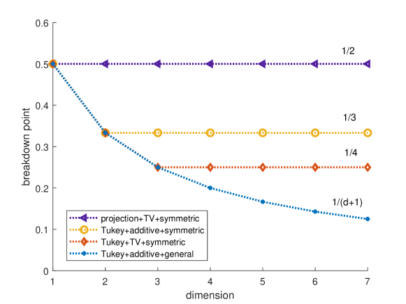
In this paper, we consider the stronger corruption model, which allows both adding and deleting mass from the original distribution. We quantify the maximum bias of Tukey median and provide both upper and lower bounds for the breakdown point under corruptions. Interestingly, the breakdown point for halfspace-symmetric distributions in high dimensions decreases from under additive corruptions to under corruptions. We show that a different algorithm, projection under the halfspace metric, has breakdown point in the same setting, which is the maximum breakdown point any translation-equivariant estimator can achieve (Rousseeuw and Leroy, 2005, Equation 1.38). We summarize the breakdown point for different algorithms in Figure 1.
We extend the population results on maximum bias and breakdown point under corruptions to the finite-sample case, showing that we approach the infinite-data limit within a constant factor once the number of samples is linear in . Our analysis holds under both the oblivious and adaptive models considered in the literature (Zhu et al., 2019).
2 Preliminaries
We provide definitions for the Tukey median, halfspace-symmetric distributions, the additive and corruption models, maximum bias, and breakdown point.
2.1 Tukey median
For any distribution and , the Tukey depth is defined as the minimum probability density on one side of a hyperplane through :
| (1) |
The Tukey median of a distribution is defined as the point(s) with largest Tukey depth:
| (2) |
When , Tukey median reduces to median. The Tukey median may not be unique even in one dimension. When the maximizer for Tukey depth is not unique, we use to denote the set for all the maximizers and refer to this set as the Tukey median for distribution .
2.2 Halfspace-symmetric distributions
We adopt the definition of halfspace-symmetric distributions from (Zuo and Serfling, 2000; Chen et al., 2002). We say a distribution is halfspace-symmetric if there exists a point such that for , and are equal in distribution for all univariate projections, i.e.
| (3) |
Here represents equal in distribution. We call the point the center of the distribution . The class of halfspace-symmetric distributions contains both the class of centro-symmetric distributions in Donoho and Gasko (1992) and elliptical distributions in Chen et al. (2018). For a halfspace-symmetric distribution , is the mean of . The Tukey depth satisfies and the Tukey median contains .
2.3 Population corruption models
In the population level, we consider two corruption models: additive corruption model and corruption model Donoho and Liu (1988); Diakonikolas et al. (2017); Zhu et al. (2019).
Additive corruption model
In a level- additive corruption model, given some true distribution , the adversary can generate corrupted distribution , where is the level of corruption, and is an arbitrary distribution selected by adversary. We denote the set for all possible -additive corruptions from as
| (4) |
Total variation distance corruption model
The total variation distance between two distributions is defined as
| (5) |
In a level- corruption model, given some true distribution , the adversary can generate any corrupted distribution with . For any , it is always true that . Thus the corruption model is a stronger corruption model than the additive corruptions, since corruptions allow not only additive corruption, but also deletion and replacement.
2.4 Maximum bias and breakdown point for Tukey median
Given a fixed distribution , the maximum bias for Tukey median is defined as the maximum distance between and , where is in the set of all possible level- corruptions:
| (6) | ||||
| (7) |
The corresponding breakdown point is defined as the minimum corruption level that can drive the maximum bias to infinity:
| (8) | ||||
| (9) |
Based on the definition of the breakdown point for a single distribution, we define the breakdown point for a family of distribution as the worst breakdown point for any distribution inside , i.e.
| (10) |
3 Population analysis of Tukey median
In this section, we quantify the maximum bias and the breakdown point of the Tukey median in population level. The maximum bias of the Tukey median for halfspace-symmetric distributions under additive corruption model is determined in (Chen et al., 2002, Theorem 3.4), which shows that the worst-case perturbation is to add a single point with mass . It is also shown in (Chen et al., 2018, Theorem 2.1) that under additive corruptions, the Tukey median achieves near optimal maximum bias for mean estimation if the true distribution belongs to the family of elliptical distributions.
Here we demonstrate a gap in the breakdown point for halfspace-symmetric distributions between the additive and corruption models.
Theorem 1.
Denote as the set of all halfspace-symmetric distributions. Then the breakdown point for is
Proof of Theorem 1.
We first show the upper bound for both breakdown points. We defer the lower bound to Theorem 2. The construction of upper bound is summarized in Figure 1.
For , by adding mass onto and letting , the maximum bias can be driven to infinity. Thus under both corruption models.
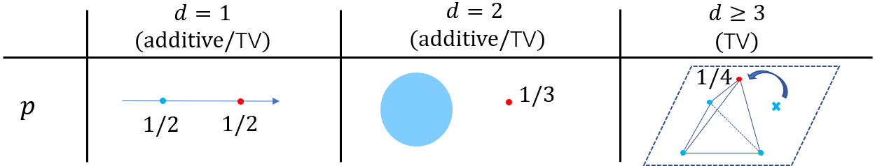
For under additive corruption model, the upper bound of breakdown point is proven in (Donoho and Gasko, 1992, Proposition 3.3). For completeness we sketch the proof here. Consider as a uniform distribution supported on unit ball. The adversary adds probability mass onto a point outside the unit ball to get a new distribution . Then . On the other hand, for any point , if is outside unit ball, there must exist a hyperplane which goes through such that the unit ball is on one side of the hyperplane. Thus . If is inside unit ball, consider any hyperplane that goes through and . The mass of the side of hyperplane which does not contain is 111If is on the same hyperplane. One can slightly rotate the hyperplane such that is not on it. This still guarantees the corresponding depth to be arbitrarily close to .. Thus we also have . Overall must be one of the Tukey median for . By setting the proof is done.
Since corruption model is a stronger corruption model, the upper bound of breakdown points for under corruptions readily follows from that under additive corruptions. Now we show the upper bound for when .
Consider the following example as illustrated in Figure 2: in a 3-dimensional space, is a distribution with equal probability on the four nodes of a 2-dimensional square. To be precise, for any . Thus is a halfspace-symmetric distribution, and gives a unique Tukey median for .
Now we move one of the point to to get corrupted distribution , where . Now the four points form a tetrahedron. For any point that is inside the tetrahedron, the Tukey depth is always . For any point that is outside the tetrahedron, the Tukey depth is always . Thus all the points inside the tetrahedron are a Tukey median for the corrupted distribution . By taking , the Tukey median is driven to infinity. Thus we know that when .
∎
Without the halfspace-symmetric assumption, the breakdown point for Tukey median under additive corruption model is , which is shown in (Donoho and Gasko, 1992, Proposition 2.3). This is also true under corruption model.
To better illustrate the behavior of Tukey median, we analyze the maximum bias for halfspace-symmetric distributions. The performance guarantee relies on the decay function of the distribution, which characterizes how much probability mass is around the center of distribution. Assume the true distribution is halfspace-symmetric centered at . We define the decay function as
| (11) |
where is the dual norm of . Note that is a non-increasing non-negative function and for halfspace-symmetric distributions.
In the next theorem, we show that the maximum bias is controlled if the distribution has enough mass around its center:
Theorem 2.
Assume is halfspace-symmetric with center and decay function defined in (11). Then the maximum bias satisfies:
| (12) | ||||
| (13) |
Here is the generalized inverse function of defined as
| (14) |
For Gaussian distribution with the operator norm of covariance bounded, is the mean and for small, and Theorem 2 implies that Tukey median achieves the maximum bias for robust Gaussian mean estimation, which is known to be optimal up to constant factor.
For any fixed distribution , it suffices to have for to be finite. Thus as a direct corollary of Theorem 2, it provides tight lower bound on the breakdown point of halfspace symmetric distributions in Theorem 1 via noting that for halfspace-symmetric distributions.
The results in Theorem 2 can be extended beyond halfspace symmetric distributions. For any true distribution , since the Tukey median of may not be unique, we define the new as
| (15) |
Then following the same argument as the proof, the result in (12) and (13) still hold.
Proof of Theorem 2.
We first show that it suffices to bound via the following lemma:
Lemma 1.
Under the same condition as Theorem 2, if , we have
| (16) |
Proof of Lemma 1.
Let . Indeed, for any such that , if , we have
| (17) |
resulting in a contradiction. Thus the lemma holds. ∎
Now it suffices to lower bound for different dimensions and different corruption models.
Under the corruption model, from the definition of and , we have for any ,
| (18) |
Under the additive corruption model, we have a tigher bound: from the definition we know that for any event . Thus
| (19) |
When , we know that for any distribution . Thus under additive corruption, under corruption.
When , we know that for any distribution from (Donoho and Gasko, 1992, Proposition 2.3). Thus following the same argument as , we have under additive corruption, under corruption.
For arbitrary dimension under additive corruption model, we also have another lower bound:
| (20) |
Here we use that for any event . For corruption model, we have
Combining the lower bounds with Lemma 1 gives the proof. ∎
4 Finite sample analysis of Tukey median
In this section, we extend the population results in the previous section to finite-sample case.
Given finite samples, there are two different corruption models: oblivious corruption and adaptive corruption (Zhu et al., 2019). In the oblivious corruption, the adversary first picks a corrupted population distribution from , then we take samples from . In the adaptive corruption, we first take samples from , then the adversary samples from some distribution that is stochastically dominated by a binomial distribution and replace points in the samples by arbitrary points to get the corrupted empirical distribution . It is shown in Diakonikolas et al. (2019); Zhu et al. (2019) that adaptive corruption model is a stronger corruption model than oblivious corruptions.
Now we bound the maximum bias in the finite-sample case. We show that with samples, the estimation error can be of the same order as the population error in Theorem 2:
Theorem 3.
Assume the true distribution is halfspace-symmetric centered at with decay function defined in (11). Denote as the corrupted empirical distribution under either oblivious or adaptive corruptions of level . When , with probability at least , there exists universal constant such that for any as the Tukey median of ,
| (21) |
when . Here , is the generalized inverse function of defined in (14).
Proof.
It suffices to show the result for adaptive corruption model. From Lemma 1, we know that it also suffices to lower bound , where .
We introduce the halfspace metric defined in Donoho and Liu (1988) as
| (22) |
From the definition we have for all . We first show that for any two distributions and any . To see this, note that the left hand side is
For Tukey median ,
Now let be the uncorrupted distribution, so that is obtained from by modifying part of samples as in adaptive corruption model. Then by triangle inequality of ,
where we repeatedly use the fact that for any , we have . Here follows adaptive corruption model. Now we upper bound the two terms and . From (Zhu et al., 2019, Lemma B.1), we know that with probability at least ,
| (23) |
For the second term , from the VC inequality (Devroye and Lugosi, 2012, Chap 2, Chapter 4.3) and the fact that the family of sets has VC dimension , there exists some universal constant such that with probability at least :
| (24) |
Denote . Combining the two lemmata together, we know that with probability at least , The proof is completed by combining the result with Lemma 1. ∎
As a direct corollary of the finite sample result, we can show that for Gaussian distribution the estimation error is with sample complexity . We remark that with the same proof, the population results in Theorem 2 for and additive corruptions can all be extended to finite-sample results with sample complexity . Similarly the halfspace-symmetric assumption can be discarded.
5 Projection Algorithm
In the previous two sections, we show that Tukey median can achieve breakdown point for halfspace symmetric distributions under corruptions and the sample complexity is linear in dimension. In this section, we show that projection under halfspace metric , as defined in (22), is able to improve the breakdown point to under the same conditions. The projection algorithm is first proposed in Donoho and Liu (1988) for robust mean estimation, and later generalized in Zhu et al. (2019) for general robust inference problems.
Denote as the set of halfspace-symmetric distributions with controlled cumulative density function around its center:
| (25) |
The projection algorithm projects the corrupted empirical distribution onto the set under distance, i.e. the output is
| (26) |
Note that the projection algorithm requires the knowledge of the set , while the Tukey median is agnostic to the distributional assumption on . In return, the projection algorithm achieves a breakdown point of and better maximum bias than the Tukey median, as shown in the following theorem:
Theorem 4.
Proof.
By triangle inequality and the property of projection,
| (28) |
We also know that . Let . We have
| (29) |
We show that it implies for any , .
For any such that , if ,
| (30) |
On the other hand, from , we know that
resulting in a contradiction.
∎
The population result can also be extended to finite-sample case by projecting instead of under . The proof follows the same technique in Theorem 3. The key to the success of projection is that it allows us to check the halfspace that goes through the middle of and , while Tukey median is only allowed to check the halfspace that goes through and . Although projection under would also give the same population rate, the finite sample error can be huge since . For both Theorem 3 and 4, the results can be extended to a more general perturbation model of corruptions under distance.
6 Open Problem
Considering the corruption model, Tukey median is an affine-equivariant estimator with breakdown point in high dimensions and good finite sample error for halfspace-symmetric distributions. The projection algorithm is not affine-equivariant, but achieves breakdown point and good finite sample error in the same set of distributions. Both algorithms may not be efficiently solvable.
It is an open problem to find an estimator that is affine-equivariant, with breakdown point and good finite sample error for halfspace-symmetric distributions without considering computational efficiency.
References
- Chen et al. [2018] Mengjie Chen, Chao Gao, and Zhao Ren. Robust covariance and scatter matrix estimation under huber’s contamination model. The Annals of Statistics, 46(5):1932–1960, 2018.
- Chen et al. [2002] Zhiqiang Chen, David E Tyler, et al. The influence function and maximum bias of tukey’s median. The Annals of Statistics, 30(6):1737–1759, 2002.
- Devroye and Lugosi [2012] Luc Devroye and Gábor Lugosi. Combinatorial methods in density estimation. Springer Science & Business Media, 2012.
- Diakonikolas et al. [2017] Ilias Diakonikolas, Gautam Kamath, Daniel M Kane, Jerry Li, Ankur Moitra, and Alistair Stewart. Being robust (in high dimensions) can be practical. In Proceedings of the 34th International Conference on Machine Learning-Volume 70, pages 999–1008. JMLR. org, 2017.
- Diakonikolas et al. [2019] Ilias Diakonikolas, Gautam Kamath, Daniel Kane, Jerry Li, Ankur Moitra, and Alistair Stewart. Robust estimators in high-dimensions without the computational intractability. SIAM Journal on Computing, 48(2):742–864, 2019.
- Donoho [1982] David L Donoho. Breakdown properties of multivariate location estimators. Technical report, Technical report, Harvard University, Boston, 1982.
- Donoho and Gasko [1992] David L Donoho and Miriam Gasko. Breakdown properties of location estimates based on halfspace depth and projected outlyingness. The Annals of Statistics, 20(4):1803–1827, 1992.
- Donoho and Liu [1988] David L Donoho and Richard C Liu. The “automatic” robustness of minimum distance functionals. The Annals of Statistics, 16(2):552–586, 1988.
- Huber [1973] Peter J Huber. Robust regression: asymptotics, conjectures and monte carlo. The Annals of Statistics, 1(5):799–821, 1973.
- Rousseeuw and Leroy [2005] Peter J Rousseeuw and Annick M Leroy. Robust regression and outlier detection, volume 589. John wiley & sons, 2005.
- Tukey [1975] John W Tukey. Mathematics and the picturing of data. In Proceedings of the International Congress of Mathematicians, Vancouver, 1975, volume 2, pages 523–531, 1975.
- Zhu et al. [2019] Banghua Zhu, Jiantao Jiao, and Jacob Steinhardt. Generalized resilience and robust statistics. arXiv preprint arXiv:1909.08755, 2019.
- Zuo and Serfling [2000] Yijun Zuo and Robert Serfling. General notions of statistical depth function. Annals of statistics, pages 461–482, 2000.