itemizestditemize
TEASER: Fast and Certifiable Point Cloud Registration
Abstract
We propose the first fast and certifiable algorithm for the registration of two sets of 3D points in the presence of large amounts of outlier correspondences. A certifiable algorithm is one that attempts to solve an intractable optimization problem (e.g., robust estimation with outliers) and provides readily checkable conditions to verify if the returned solution is optimal (e.g., if the algorithm produced the most accurate estimate in the face of outliers) or bound its sub-optimality or accuracy.
Towards this goal, we first reformulate the registration problem using a Truncated Least Squares (TLS) cost that makes the estimation insensitive to a large fraction of spurious correspondences. Then, we provide a general graph-theoretic framework to decouple scale, rotation, and translation estimation, which allows solving in cascade for the three transformations. Despite the fact that each subproblem (scale, rotation, and translation estimation) is still non-convex and combinatorial in nature, we show that (i) TLS scale and (component-wise) translation estimation can be solved in polynomial time via an adaptive voting scheme, (ii) TLS rotation estimation can be relaxed to a semidefinite program (SDP) and the relaxation is tight, even in the presence of extreme outlier rates, and (iii) the graph-theoretic framework allows drastic pruning of outliers by finding the maximum clique. We name the resulting algorithm TEASER (Truncated least squares Estimation And SEmidefinite Relaxation). While solving large SDP relaxations is typically slow, we develop a second fast and certifiable algorithm, named TEASER++, that uses graduated non-convexity to solve the rotation subproblem and leverages Douglas-Rachford Splitting to efficiently certify global optimality.
For both algorithms, we provide theoretical bounds on the estimation errors, which are the first of their kind for robust registration problems. Moreover, we test their performance on standard benchmarks, object detection datasets, and the 3DMatch scan matching dataset, and show that (i) both algorithms dominate the state of the art (e.g., RANSAC, branch-&-bound, heuristics) and are robust to more than outliers when the scale is known, (ii) TEASER++ can run in milliseconds and it is currently the fastest robust registration algorithm, and (iii) TEASER++ is so robust it can also solve problems without correspondences (e.g., hypothesizing all-to-all correspondences) where it largely outperforms ICP and it is more accurate than Go-ICP while being orders of magnitude faster. We release a fast open-source C++ implementation of TEASER++.
Index Terms:
3D registration, scan matching, point cloud alignment, robust estimation, certifiable algorithms, outliers-robust estimation, object pose estimation, 3D robot vision.Supplementary Material
-
•
Video: https://youtu.be/xib1RSUoeeQ
- •
I Introduction
| Correspondence-based |
 (a) Input
|
 (b) RANSAC
|
 (c) TEASER++
|
| Correspondence-free |
 (d) Input
|
 (e) ICP
|
 (f) TEASER++
|
| Object Localization |
 (g) Correspondences
|
 (h) TEASER++
|
| Scan Matching |
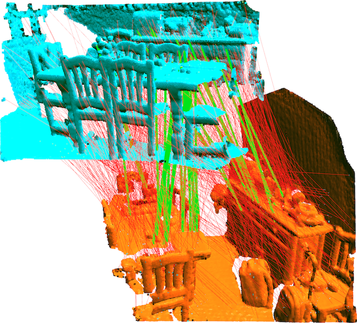 (i) Correspondences
|
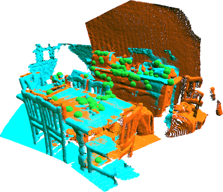 (j) TEASER++
|
Point cloud registration (also known as scan matching or point cloud alignment) is a fundamental problem in robotics and computer vision and consists in finding the best transformation (rotation, translation, and potentially scale) that aligns two point clouds. It finds applications in motion estimation and 3D reconstruction [3, 4, 5, 6], object recognition and localization [7, 8, 9, 10], panorama stitching [11], and medical imaging [12, 13], to name a few.
When the ground-truth correspondences between the point clouds are known and the points are affected by zero-mean Gaussian noise, the registration problem can be readily solved, since elegant closed-form solutions [14, 15] exist for the case of isotropic noise. In practice, however, the correspondences are either unknown, or contain many outliers, leading these solvers to produce poor estimates. Large outlier rates are typical of 3D keypoint detection and matching [16].
Commonly used approaches for registration with unknown or uncertain correspondences either rely on the availability of an initial guess for the unknown transformation (e.g., the Iterative Closest Point, ICP [17]), or implicitly assume the presence of a small set of outliers (e.g., RANSAC [18]111RANSAC’s runtime grows exponentially with the outlier ratio [19] and it typically performs poorly with large outlier rates (see Sections II and XI).). These algorithms may fail without notice (Fig. 1 (b),(e)) and may return estimates that are arbitrarily far from the ground-truth transformation. In general, the literature is divided between heuristics, that are fast but brittle, and global methods that are guaranteed to be robust, but run in worst-case exponential time (e.g., branch-&-bound methods, such as Go-ICP [20]).
This paper is motivated by the goal of designing an approach that (i) can solve registration globally (without relying on an initial guess), (ii) can tolerate extreme amounts of outliers (e.g., when of the correspondences are outliers), (iii) runs in polynomial time and is fast in practice (i.e., can operate in real-time on a robot), and (iv) provides formal performance guarantees. In particular, we look for a posteriori guarantees, e.g., conditions that one can check after executing the algorithm to assess the quality of the estimate. This leads to the notion of certifiable algorithms, i.e., an algorithm that attempts to solve an intractable problem and provides checkable conditions on whether it succeeded [21, 22, 23, 24, 25, 26]. The interested reader can find a broader discussion in Appendix A.
Contribution. This paper proposes the first certifiable algorithm for 3D registration with outliers. We reformulate the registration problem using a Truncated Least Squares (TLS) cost (presented in Section IV), which is insensitive to a large fraction of spurious correspondences but leads to a hard, combinatorial, and non-convex optimization.
The first contribution (Section V) is a general framework to decouple scale, rotation, and translation estimation. The idea of decoupling rotation and translation has appeared in related work, e.g., [27, 28, 19]. The novelty of our proposal is fourfold: (i) we develop invariant measurements to estimate the scale ([28, 19] assume the scale is given), (ii) we make the decoupling formal under the assumption of unknown-but-bounded noise [29, 30], (iii) we provide a general graph-theoretic framework to derive these invariant measurements, and (iv) we show that this framework allows pruning a large amount of outliers by finding the maximum clique of the graph defined by the invariant measurements (Section VI).
The decoupling allows solving in cascade for scale, rotation, and translation. However, each subproblem is still combinatorial in nature. Our second contribution is to show that (i) in the scalar case TLS estimation can be solved exactly in polynomial time using an adaptive voting scheme, and this enables efficient estimation of the scale and the (component-wise) translation (Section VII); (ii) we can formulate a tight semidefinite programming (SDP) relaxation to estimate the rotation and establish a posteriori conditions to check the quality of the relaxation (Section VIII). We remark that the rotation subproblem addressed in this paper is in itself a foundational problem in vision (where it is known as rotation search [31]) and aerospace (where it is known as the Wahba problem [32]). Our SDP relaxation is the first certifiable algorithm for robust rotation search.
Our third contribution (Section IX) is a set of theoretical results certifying the quality of the solution returned by our algorithm, named Truncated least squares Estimation And SEmidefinite Relaxation (TEASER). In the noiseless case, we provide easy-to-check conditions under which TEASER recovers the true transformation between the point clouds in the presence of outliers. In the noisy case, we provide bounds on the distance between the ground-truth transformation and TEASER’s estimate. To the best of our knowledge these are the first non-asymptotic error bounds for geometric estimation problems with outliers, while the literature on robust estimation in statistics (e.g., [33]) typically studies simpler problems in Euclidean space and focuses on asymptotic bounds.
Our fourth contribution (Section X) is to implement a fast version of TEASER, named TEASER++, that uses graduated non-convexity (GNC) [34] to estimate the rotation without solving a large SDP. We show that TEASER++ is also certifiable, and in particular we leverage Douglas-Rachford Splitting [35] to design a scalable optimality certifier that can assert global optimality of the estimate returned by GNC. We release a fast open-source C++ implementation of TEASER++.
Our last contribution (Section XI) is an extensive evaluation in both standard benchmarks and on real datasets for object detection [36] and scan matching [37]. In particular, we show that (i) both TEASER and TEASER++ dominate the state of the art (e.g., RANSAC, branch-&-bound, heuristics) and are robust to more than outliers when the scale is known, (ii) TEASER++ can run in milliseconds and it is currently the fastest robust registration algorithm, (iii) TEASER++ is so robust it can also solve problems without correspondences (e.g., hypothesizing all-to-all correspondences) where it largely outperforms ICP and it is more accurate than Go-ICP while being orders of magnitude faster, and (iv) TEASER++ can boost registration performance when combined with deep-learned keypoint detection and matching.
Novelty with respect to [38, 39]. In our previous works, we introduced TEASER [38] and the quaternion-based relaxation of the rotation subproblem [39] (named QUASAR). The present manuscript brings TEASER to maturity by (i) providing explicit theoretical results on TEASER’s performance (Section IX), (ii) providing a fast optimality certification method (Section VIII-C), (iii) developing a fast algorithm, TEASER++, that uses GNC to estimate the rotation without solving an SDP, while still being certifiable (Section X), and (iv) reporting a more comprehensive experimental evaluation, including real tests on the 3DMatch dataset and examples of registration without correspondences (Sections XI-C and XI-E). These are major improvements both on the theoretical side ([38, 39] only certified performance on each subproblem, rather than end-to-end, and required solving a large SDP) and on the practical side (TEASER++ is more than three orders of magnitude faster than our proposal in [38]).
II Related Work
There are two popular paradigms for the registration of 3D point clouds: Correspondence-based and Simultaneous Pose and Correspondence (i.e., correspondence-free) methods.
II-A Correspondence-based Methods
Correspondence-based methods first detect and match 3D keypoints between point clouds using feature descriptors [16, 1, 7, 40], and then use an estimator to infer the transformation from these putative correspondences. 3D keypoint matching is known to be less accurate compared to 2D counterparts like SIFT and ORB, thus causing much higher outlier rates, e.g., having 95% spurious correspondences is considered common [19]. Therefore, a robust backend that can deal with extreme outlier rates is highly desirable.
Registration without Outliers. Horn [14] and Arun [15] show that optimal solutions (in the maximum likelihood sense) for scale, rotation, and translation can be computed in closed form when the correspondences are known and the points are affected by isotropic zero-mean Gaussian noise. Olsson et al. [41] propose a method based on Branch-&-bound (BnB) that is globally optimal and allows point-to-point, point-to-line, and point-to-plane correspondences. Briales and Gonzalez-Jimenez [42] propose a tight semidefinite relaxation to solve the same registration problem as in [41].
If the two sets of points only differ by an unknown rotation (i.e., we do not attempt to estimate the scale and translation), we obtain a simplified version of the registration problem that is known as rotation search in computer vision [31], or Wahba problem in aerospace [32]. In aerospace, the vector observations are typically the directions to visible stars observed by sensors onboard the satellite. Closed-form solutions to the Wahba problem are known using both quaternion [14, 43] and rotation matrix [44, 15] representations. The Wahba problem is also related to the well-known Orthogonal Procrustes problem [45] where one searches for orthogonal matrices (rather than rotations), for which a closed-form solution also exists [46]. The computer vision community has investigated the rotation search problem in the context of point cloud registration [17, 20], image stitching [11], motion estimation and 3D reconstruction [4, 5]. In particular, the closed-form solutions from Horn [14] and Arun et al. [15] can be used for (outlier-free) rotation search with isotropic Gaussian noise. Ohta and Kanatani [47] propose a quaternion-based optimal solution, and Cheng and Crassidis [48] develop a local optimization algorithm, for the case of anisotropic Gaussian noise. Ahmed et al. [49] develop an SDP relaxation for the case with bounded noise and no outliers.
Robust Registration. Probably the most widely used robust registration approach is based on RANSAC [18], which has enabled several early applications in vision and robotics [50, 51]. Despite its efficiency in the low-noise and low-outlier regime, RANSAC exhibits slow convergence and low accuracy with large outlier rates [19], where it becomes harder to sample a “good” consensus set. Other approaches resort to M-estimation, which replaces the least squares objective function with robust costs that are less sensitive to outliers [52, 53, 54]. Zhou et al. [55] propose Fast Global Registration (FGR) that uses the Geman-McClure cost function and leverages graduated non-convexity to solve the resulting non-convex optimization. Despite its efficiency, FGR offers no optimality guarantees. Indeed, FGR tends to fail when the outlier ratio is high (>80%), as we show in Section XI. Enqvist et al. [56] propose to optimally find correct correspondences by solving the vertex cover problem and demonstrate robustness against over outliers in 3D registration. Parra and Chin [19] propose a Guaranteed Outlier REmoval (GORE) technique, that uses geometric operations to significantly reduce the amount of outlier correspondences before passing them to the optimization backend. GORE has been shown to be robust to 95% spurious correspondences [19]. In an independent effort, Parra et al. [57] find pairwise-consistent correspondences in 3D registration using a practical maximum clique (PMC) algorithm. While similar in spirit to our original proposal [38], both GORE and PMC do not estimate the scale of the registration and are typically slower since they rely on BnB (see Algorithm 2 in [19]). Yang and Carlone [38] propose the first certifiable algorithm for robust registration, which however requires solving a large-scale SDP hence being limited to small problems. Recently, physics-based registration has been proposed in [58, 59, 60].
Similar to the registration problem, rotation search with outliers has also been investigated in the computer vision community. Local techniques for robust rotation search are again based on RANSAC or M-estimation, but are brittle and do not provide performance guarantees. Global methods (that guarantee to compute globally optimal solutions) are based on Consensus Maximization [61, 62, 63, 64, 65, 66] and BnB [67]. Hartley and Kahl [31] first proposed using BnB for rotation search, and Bazin et al. [68] adopted consensus maximization to extend their BnB algorithm with a robust formulation. BnB is guaranteed to return the globally optimal solution, but it runs in exponential time in the worst case. Another class of global methods for Consensus Maximization enumerates all possible subsets of measurements with size no larger than the problem dimension (3 for rotation search) to analytically compute candidate solutions, and then verify global optimality using computational geometry [69, 70]. Similarly, Ask et al. [71] show the TLS estimation can also be solved globally by enumerating subsets with size no larger than the model dimension. However, these methods require exhaustive enumeration and become intractable when the problem dimension is large (e.g., for 3D registration). In [39], we propose the first quaternion-based certifiable algorithm for robust rotation search (reviewed in Section VIII).
II-B Simultaneous Pose and Correspondence Methods
Simultaneous Pose and Correspondence (SPC) methods alternate between finding the correspondences and computing the best transformation given the correspondences.
Local Methods. The Iterative Closest Point (ICP) algorithm [17] is considered a milestone in point cloud registration. However, ICP is prone to converge to local minima and only performs well given a good initial guess. Multiple variants of ICP [72, 73, 74, 75] have proposed to use robust cost functions to improve convergence. Probabilistic interpretations have also been proposed to improve ICP as a minimization of the Kullback-Leibler divergence between two Mixture models [76, 77]. Clark et al. [78] alignn point clouds as continuous functions using Riemannian optimization. Le et al. [79] use semidefinite relaxation to generate hypotheses for randomized methods. All these methods do not provide global optimality guarantees.
Global Methods. Global SPC approaches compute a globally optimal solution without initial guesses, and are usually based on BnB. A series of geometric techniques have been proposed to improve the bounding tightness [31, 80, 20, 81] and increase the search speed [82, 20]. However, the runtime of BnB increases exponentially with the size of the point cloud and is made worse by the explosion of the number of local minima resulting from high outlier ratios [19]. Global SPC registration can be also formulated as a mixed-integer program [83], though the runtime remains exponential. Maron et al. [84] design a tight semidefinite relaxation, which, however, only works for SPC registration with full overlap.
Deep Learning Methods. The success of deep learning on 3D point clouds (e.g., PointNet [85] and DGCNN [86]) opens new opportunities for learning point cloud registration from data. Deep learning methods first learn to embed points clouds in a high-dimensional feature space, then learn to match keypoints to generate correspondences, after which optimization over the space of rigid transformations is performed for the best alignment. PointNetLK [87] uses PointNet to learn feature representations and then iteratively align the features representations, instead of the 3D coordinates. DCP [88] uses DGCNN features for correspondence matching and Horn’s method for registration in an end-to-end fashion (Horn’s method is differentiable). PRNet [89] extends DCP to aligning partially overlapping point clouds. Scan2CAD [90] and its improvement [91] apply similar pipelines to align CAD models to RGB-D scans. 3DSmoothNet [2] uses a siamese deep learning architecture to establish keypoint correspondences between two point clouds. FCGF [40] leverages sparse high-dimensional convolutions to extract dense feature descriptors from point clouds. Deep global registration [92] uses FCGF feature descriptors for point cloud registration. In Section XI-E we show that (i) our approach provides a robust back-end for deep-learned keypoint matching algorithms (we use [2]), and (ii) that current deep learning approaches still struggle to produce acceptable inlier rates in real problems.
Remark 1 (Reconciling Correspondence-based and SPC Methods).
Correspondence-based and SPC methods are tightly coupled. First of all, approaches like ICP alternate between finding the correspondences and solving a correspondence-base problem. More importantly, one can always reformulate an SPC problem as a correspondence-based problem by hypothesizing all-to-all correspondences, i.e., associating each point in the first point cloud to all the points in the second. To the best of our knowledge, only [56, 93] have pursued this formulation since it leads to an extreme number of outliers. In this paper, we show that our approach can indeed solve the SPC problem thanks to its unprecedented robustness to outliers (Section XI-C).
III Notations and Preliminaries
Scalars, Vectors, Matrices. We use lowercase characters (e.g., ) to denote real scalars, bold lowercase characters (e.g., ) for real vectors, and bold uppercase characters (e.g., ) for real matrices. denotes the -th row and -th column scalar entry of matrix , and (or simply when is clear from the context) denotes the -th row and -th column block of the matrix . is the identity matrix of size . We use “” to denote the Kronecker product. For a square matrix , and denote its determinant and trace. The 2-norm of a vector is denoted as . The Frobenious norm of a matrix is denoted as . For a symmetric matrix of size , we use to denote its real eigenvalues.
Sets. We use calligraphic fonts to denote sets (e.g., ). We use (resp. ) to denote the group of real symmetric (resp. skew-symmetric) matrices with size . denotes the set of symmetric positive semidefinite matrices. denotes the -dimensional special orthogonal group, while denotes the -dimensional unit sphere.
Quaternions. Unit quaternions are a representation for a 3D rotation . We denote a unit quaternion as a unit-norm column vector , where is the vector part of the quaternion and the last element is the scalar part. We also use to denote the four entries of the quaternion. Each quaternion represents a 3D rotation and the composition of two rotations and can be computed using the quaternion product :
| (1) |
where and are defined as follows:
| (2) |
The inverse of a quaternion is defined as , where one simply reverses the sign of the vector part. The rotation of a vector can be expressed in terms of quaternion product. Formally, if is the (unique) rotation matrix corresponding to a unit quaternion , then:
| (5) |
where is the homogenization of , obtained by augmenting with an extra entry equal to zero. The set of unit quaternions, i.e., the -dimensional unit sphere , is a double cover of since and represent the same rotation (this fact can be easily seen by examining eq. (5)).
IV Robust Registration with
Truncated Least Squares Cost
In the robust registration problem, we are given two 3D point clouds and , with . We consider a correspondence-based setup, where we are given putative correspondences , that obey the following generative model:
| (6) |
where , , and are the unknown (to-be-computed) scale, rotation, and translation, models the measurement noise, and is a vector of zeros if the pair is an inlier, or a vector of arbitrary numbers for outlier correspondences. In words, if the -th correspondence is an inlier correspondence, corresponds to a 3D transformation of (plus noise ), while if is an outlier correspondence, is just an arbitrary vector.
Registration without Outliers. When is a zero-mean Gaussian noise with isotropic covariance , and all the correspondences are correct (i.e., ), the Maximum Likelihood estimator of can be computed by solving the following nonlinear least squares problem:
| (7) |
Although (7) is a non-convex problem, due to the non-convexity of the set , its optimal solution can be computed in closed form by decoupling the estimation of the scale, rotation, and translation, using Horn’s [14] or Arun’s method [15]. A key contribution of the present paper is to provide a way to decouple scale, rotation, and translation in the more challenging case with outliers.
In practice, a large fraction of the correspondences are outliers, due to incorrect keypoint matching. Despite the elegance of the closed-form solutions [14, 15], they are not robust to outliers, and a single “bad” outlier can compromise the correctness of the resulting estimate. Hence, we propose a truncated least squares registration formulation that can tolerate extreme amounts of spurious data.
Truncated Least Squares Registration. We depart from the Gaussian noise model and assume the noise is unknown but bounded [29]. Formally, we assume the inlier noise in (6) is such that , where is a given bound.
Then we adopt the following Truncated Least Squares (TLS) Registration formulation:
| (8) |
which computes a least squares solution of measurements with small residuals (), while discarding measurements with large residuals (when the -th summand becomes a constant and does not influence the optimization). Note that one can always divide each summand in (8) by : therefore, one can safely assume to be . For the sake of generality, in the following we keep since it provides a more direct “knob” to be stricter or more lenient towards potential outliers.
The noise bound is fairly easy to set in practice and can be understood as a “3-sigma” noise bound or as the maximum error we expect from an inlier. The interested reader can find a more formal discussion on how to set and in Appendix B. We remark that while we assume to have a bound on the maximum error we expect from the inliers (), we do not make assumptions on the generative model for the outliers, which is typically unknown in practice.
Remark 2 (TLS vs. Consensus Maximization).
TLS estimation is related to Consensus Maximization [61], a popular robust estimation approach in computer vision. Consensus Maximization looks for an estimate that maximizes the number of inliers, while TLS simultaneously computes a least squares estimate for the inliers. The two methods are not guaranteed to produce the same choice of inliers in general, since TLS also penalizes inliers with large errors. Appendix C provides a toy example to illustrate the potential mismatch between the two techniques and provides necessary conditions under which the two formulations find the same set of inliers.
Despite being insensitive to outlier correspondences, the truncated least squares formulation (8) is much more challenging to solve globally, compared to the outlier-free case (7). This is the case even in simpler estimation problems where the feasible set of the unknowns is convex, as stated below.
Remark 3 states the NP-hardness of TLS estimation over a convex feasible set. The TLS problem (8) is even more challenging due to the non-convexity of . While problem (8) is hard to solve directly, in the next section, we show how to decouple the estimation of scale, rotation, and translation using invariant measurements.
V Decoupling Scale, Rotation,
and Translation Estimation
We propose a general approach to decouple the estimation of scale, translation, and rotation in problem (8). The key insight is that we can reformulate the measurements (6) to obtain quantities that are invariant to a subset of the transformations (scaling, rotation, translation).
V-A Translation Invariant Measurements (TIMs)
While the absolute positions of the points in depend on the translation , the relative positions are invariant to . Mathematically, given two points and from (6), the relative position of these two points is:
| (9) |
where the translation cancels out in the subtraction. Therefore, we can obtain a Translation Invariant Measurement (TIM) by computing and , and the TIM satisfies the following generative model:
| (TIM) |
where is zero if both the -th and the -th measurements are inliers (or arbitrary otherwise), while is the measurement noise. It is easy to see that if and , then .
The advantage of the TIMs in eq. (TIM) is that their generative model only depends on two unknowns, and . The number of TIMs is upper-bounded by , where pairwise relative measurements between all pairs of points are computed. Theorem 4 below connects the TIMs with the topology of a graph defined over the 3D points.
Theorem 4 (Translation Invariant Measurements).
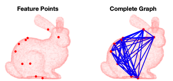
Define the vectors (resp. ), obtained by concatenating all vectors (resp. ) in a single column vector. Moreover, define an arbitrary graph with nodes and an arbitrary set of edges . Then, the vectors and are TIMs, where is the incidence matrix of [96].
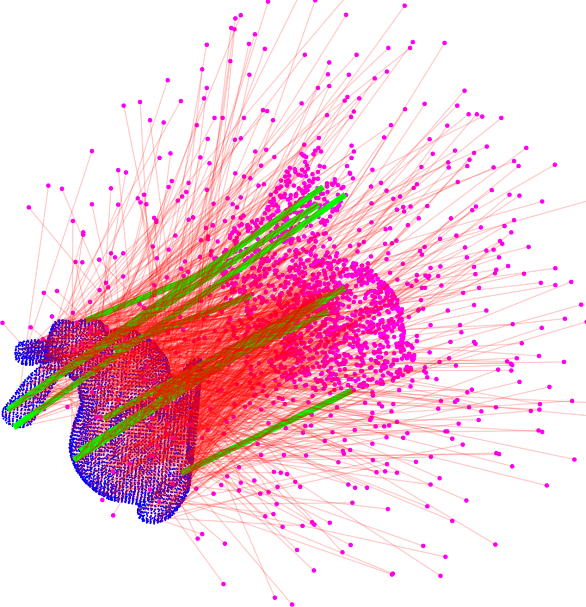
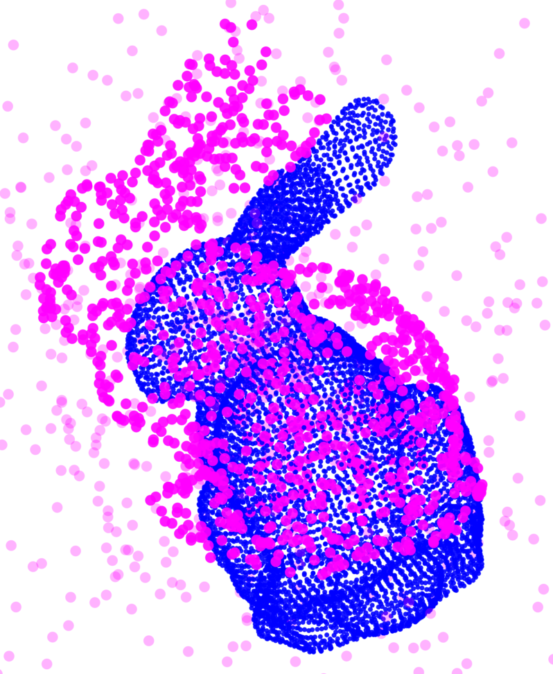
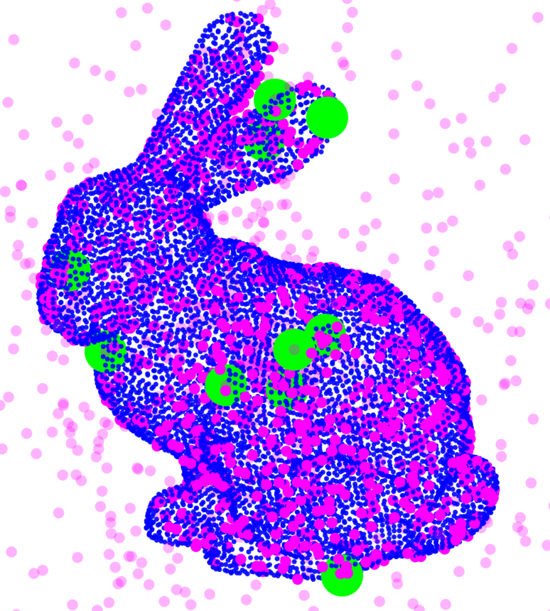
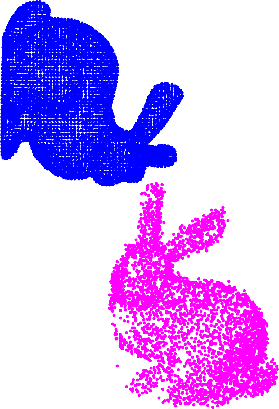
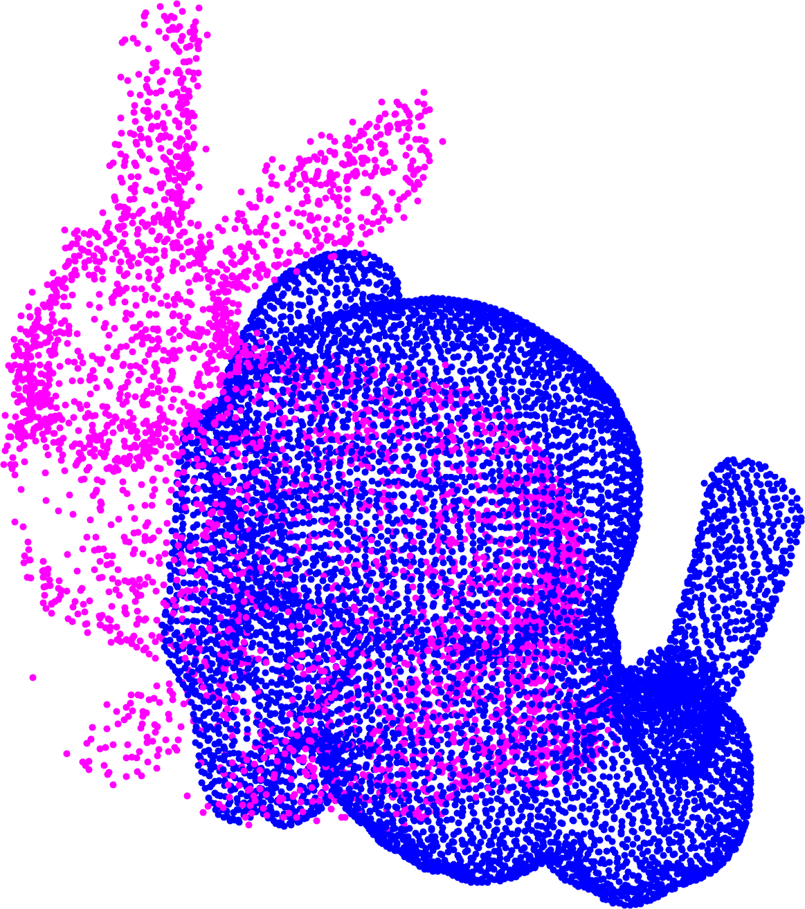
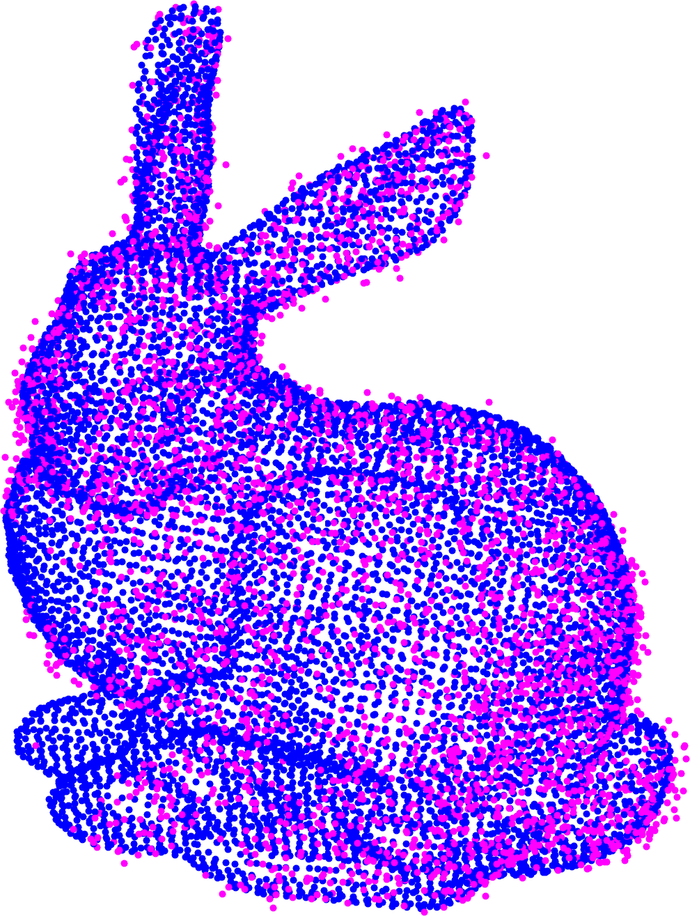
A proof of the theorem is given in Appendix D. TIMs generated from a complete graph on the Bunny dataset [97] are illustrated in Fig. 2.
V-B Translation and Rotation Invariant Measurements (TRIMs)
While the relative locations of pairs of points (TIMs) still depend on the rotation , their distances are invariant to both and . Therefore, to build rotation invariant measurements, we compute the norm of each TIM vector:
| (10) |
We now note that for the inliers () it holds (using and the triangle inequality):
| (11) |
hence we can write (10) equivalently as:
| (12) |
with , and if both and are inliers or is an arbitrary scalar otherwise. Recalling that the norm is rotation invariant and that , and dividing both sides of (12) by , we obtain new measurements :
| (TRIM) |
where , and . It is easy to see that since . We define .
Eq. (TRIM) describes a Translation and Rotation Invariant Measurement (TRIM) whose generative model is only function of the unknown scale .
Remark 5 (Novelty of Invariant Measurements).
Ideas similar to the translation invariant measurements (TIMs) have been used in recent work [98, 19, 28, 99, 100] while (i) the novel graph-theoretic interpretation of Theorem 4 generalizes previously proposed methods and allows pruning outliers as described in Section VI-D, and (ii) the notion of translation and rotation invariant measurements (TRIMs) is completely new. We also remark that while related work uses invariant measurements to filter-out outliers [19] or to speed up BnB [98, 28], we show that they also allow decoupling the estimation of scale, rotation, and translation.
A summary table of the invariant measurements and the corresponding noise bounds is given in Appendix E.
VI Truncated least squares Estimation And SEmidefinite Relaxation (TEASER): Overview
We propose a decoupled approach to solve in cascade for the scale, the rotation, and the translation in (8). The approach, named Truncated least squares Estimation And SEmidefinite Relaxation (TEASER), works as follows:
-
1.
we use the TRIMs to estimate the scale
-
2.
we use and the TIMs to estimate the rotation
-
3.
we use and to estimate the translation from in the original TLS problem (8).
We state each subproblem in the following subsections.
VI-A Robust Scale Estimation
The generative model (TRIM) describes linear scalar measurements of the unknown scale , affected by bounded noise including potential outliers (when ). Again, we estimate the scale given the measurements and the bounds using a TLS estimator:
VI-B Robust Rotation Estimation
Given the scale estimate produced by the scale estimation, the generative model (TIM) describes measurements affected by bounded noise including potential outliers (when ). Again, we compute from the estimated scale , the TIM measurements and the bounds using a TLS estimator:
| (14) |
where for simplicity we numbered the measurements from to and adopted the notation instead of . Problem (14) is known as the Robust Wahba or Robust Rotation Search problem [39]. Section VIII shows that (14) can be solved exactly and in polynomial time (in practical problems) via a tight semidefinite relaxation.
VI-C Robust Component-wise Translation Estimation
After obtaining the scale and rotation estimates and by solving (13)-(14), we can substitute them back into problem (8) to estimate the translation . Although (8) operates on the norm of the vector, we propose to solve for the translation component-wise, i.e., we compute the entries of independently:
| (15) |
for , and where denotes the -th entry of a vector. Since is a known vector in this stage, it is easy to see that (15) is a scalar TLS problem. Therefore, similarly to (13), Section VII shows that (15) can be solved exactly and in polynomial time via adaptive voting (Algorithm 2). The interested reader can find a discussion on component-wise versus full TLS translation estimation in Appendix Q,
VI-D Boosting Performance: Max Clique Inlier Selection (MCIS)
While in principle we could simply execute the cascade of scale, rotation, and translation estimation described above, our graph-theoretic interpretation of Theorem 4 affords further opportunities to prune outliers.
Consider the TRIMs as edges in the complete graph (where the vertices are the correspondences and the edge set induces the TIMs and TRIMs per Theorem 4). After estimating the scale (13) (discussed in Section VII), we can prune the edges in the graph whose associated TRIM have been classified as outliers by the TLS formulation (i.e., ). This allows us to obtain a pruned graph , with , where gross outliers are discarded. The following result ensures that inliers form a clique in the graph , enabling an even more substantial rejection of outliers.
Theorem 6 (Maximal Clique Inlier Selection).
Edges corresponding to inlier TIMs form a clique in , and there is at least one maximal clique in that contains all the inliers.
A proof of Theorem 6 is presented in Appendix F. Theorem 6 allows us to prune outliers by finding the maximal cliques of . Similar idea has been explored for rigid body motion segmentation [101]. Although finding the maximal cliques of a graph takes exponential time in general, there exist efficient approximation algorithms that scale to graphs with millions of nodes [102, 103, 104]. Under high outlier rates, the graph is sparse and the maximal clique problem can be solved quickly in practice [105]. Therefore, in this paper, after performing scale estimation and removing the corresponding gross outliers, we compute the maximal clique with largest cardinality, i.e., the maximum clique, as the inlier set to pass to rotation estimation. Section XI-A shows that this method drastically reduces the number of outliers.
VI-E Pseudocode of TEASER
The pseudocode of TEASER is summarized in Algorithm 1.
VII Robust Scale and Translation Estimation:
Adaptive Voting
In this section, we propose an adaptive voting algorithm to solve exactly the robust scale estimation and the robust component-wise translation estimation.
VII-A Adaptive Voting for Scalar TLS Estimation
Both the scale estimation (13) and the component-wise translation estimation (15) resort to finding a TLS estimate of an unknown scalar given a set of outlier-corrupted measurements. Using the notation for scale estimation (13), the following theorem shows that one can solve scalar TLS estimation in polynomial time by a simple enumeration.
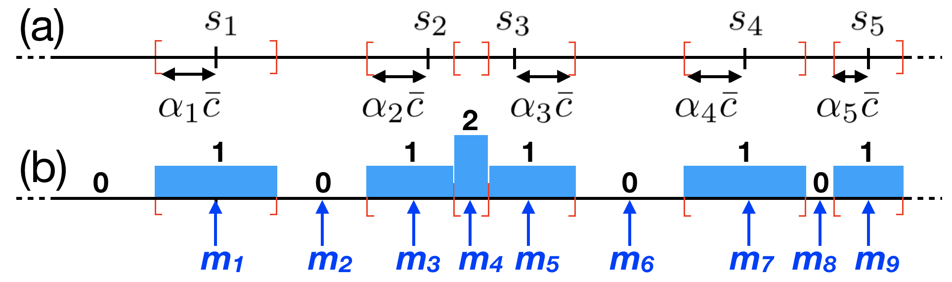
Theorem 7 (Optimal Scalar TLS Estimation).
Theorem 7, whose proof is given in Appendix G, is based on the insight that the consensus set can only change at the boundaries of the intervals (Fig. 3(a)) and there are at most such boundaries. The theorem also suggests a straightforward adaptive voting algorithm to solve (13), with pseudocode given in Algorithm 2. The algorithm first builds the boundaries of the intervals shown in Fig. 3(a) (line 2). Then, for each interval, it evaluates the consensus set (line 2, see also Fig. 3(b)). Since the consensus set does not change within an interval, we compute it at the interval centers (line 2, see also Fig. 3(b)). Finally, the cost of each consensus set is computed and the smallest cost is returned as optimal solution (line 2).
Remark 8 (Adaptive Voting).
The adaptive voting algorithm generalizes the histogram voting method of Scaramuzza [106] (i) to adaptively adjust the bin size in order to obtain an optimal solution and (ii) to solve a TLS (rather than Consensus Maximization) formulation. Adaptive voting can be also used for Consensus Maximization, by simply returning the largest consensus set in Algorithm 2. We also refer the interested reader to the paper of Liu and Jiang [94], who recently developed a similar algorithm in an independent effort and provide a generalization to 2D TLS estimation problems.
In summary, the function in Algorithm 1 calls Algorithm 2 to compute the optimal scale estimate , and the function in Algorithm 1 calls Algorithm 2 three times (one for each entry of ) and returns the translation estimate .
VIII Robust Rotation Estimation:
Semidefinite Relaxation and Fast Certificates
This section describes how to compute an optimal solution to problem (14) or certify that a given rotation estimate is globally optimal. TLS estimation is NP-hard according to Remark 3 and the robust rotation estimation (14) has the additional complexity of involving a non-convex domain (i.e., ). This section provides a surprising result: we can compute globally optimal solutions to (3) (or certify that a given estimate is optimal) in polynomial time in virtually all practical problems using a tight semidefinite (SDP) relaxation. In other words, while the NP-hardness implies the presence of worst-case instances that are not solvable in polynomial time, these instances are not observed to frequently occur in practice.
We achieve this goal in three steps. First, we show that the robust rotation estimation problem (14) can be reformulated as a Quadratically Constrained Quadratic Program (QCQP) by adopting a quaternion formulation and using a technique we name binary cloning (Section VIII-A). Second, we show how to obtain a semidefinite relaxation and relax the non-convex QCQP into a convex SDP with redundant constraints (Section VIII-B). The SDP relaxation enables solving (14) with global optimality guarantees in polynomial time. Third, we show that the relaxation also enables a fast optimality certifier, which, given a rotation guess, can test if the rotation is the optimal solution to (14) (Section VIII-C). The latter will be instrumental in developing a fast and certifiable registration approach that circumvents the time-consuming task of solving a large relaxation with existing SDP solvers. The derivation in Sections VIII-A and VIII-B is borrowed from our previous work [39], while the fast certification in Section VIII-C has not been presented before.
VIII-A Robust Rotation Estimation as a QCQP
This section rewrites problem (5) as a Quadratically Constrained Quadratic Program (QCQP). Using the quaternion preliminaries introduced in Section III –and in particular eq. (5)– it is easy to rewrite (14) using unit quaternions:
| (17) |
where we defined and , and “” denotes the quaternion product. The main advantage of using (17) is that we replaced the set with a simpler set, the -dimensional unit sphere .
From TLS to Mixed-Integer Programming. Problem (17) is hard to solve globally, due to the non-convexity of both the cost function and the domain . As a first step towards obtaining a QCQP, we expose the non-convexity of the cost by rewriting the TLS cost using binary variables. In particular, we rewrite the inner “” in (17) using the following property, that holds for any pair of scalars and :
| (18) |
Eq. (18) can be verified to be true by inspection: the right-hand-side returns (with minimizer ) if , and (with minimizer ) if . This enables us to rewrite problem (17) as a mixed-integer program including the quaternion and binary variables :
| (19) |
The reformulation is related to the Black-Rangarajan duality between robust estimation and line processes [53]: the TLS cost is an extreme case of robust function that results in a binary line process. Intuitively, the binary variables in problem (19) decide whether a given measurement is an inlier () or an outlier (). Exposing the non-convexity of TLS cost function using binary variables makes the TLS cost more favorable than other non-convex robust costs (e.g., the Geman-McClure cost used in FGR [55]), because it enables binary cloning (Proposition 9) and semidefinite relaxation (Section VIII-B).
From Mixed-Integer to Quaternions. Now we convert the mixed-integer program (19) to an optimization over quaternions. The intuition is that, if we define extra quaternions , we can rewrite (19) as a function of and (). This is a key step towards getting a quadratic cost (Proposition 10) and is formalized as follows.
Proposition 9 (Binary Cloning).
The mixed-integer program (19) is equivalent (in the sense that they admit the same optimal solution ) to the following optimization:
| (20) | |||||
which involves quaternions ( and , ).
While a formal proof is given in Appendix H, it is fairly easy to see that if , or equivalently, with , then , and which exposes the relation between (19) and (20). We dubbed the re-parametrization (20) binary cloning since now we created a “clone” for each measurement, such that for inliers (recall ) and for outliers.
From Quaternions to QCQP. We conclude this section by showing that (20) can be actually written as a QCQP. This observation is non-trivial since (20) has a quartic cost and is not in the form of a quadratic constraint. The re-formulation as a QCQP is given in the following.
Proposition 10 (Binary Cloning as a QCQP).
Define a single column vector stacking all variables in Problem (20). Then, Problem (20) is equivalent (in the sense that they admit the same optimal solution ) to the following Quadratically-Constrained Quadratic Program:
| (21) | |||||
| s.t. | |||||
where is a known symmetric matrix that depends on the TIM measurements and (the explicit expression is given in Appendix I), and the notation (resp. ) denotes the 4D subvector of corresponding to (resp. ).
A complete proof of Proposition 10 is given in Appendix I. Intuitively, (i) we developed the squares in the cost function (20), (ii) we used the properties of unit quaternions (Section III) to simplify the expression to a quadratic cost, and (iii) we adopted the more compact notation afforded by the vector to obtain (21).
VIII-B Semidefinite Relaxation
Problem (21) writes the TLS rotation estimation problem (14) as a QCQP. Problem (21) is still a non-convex problem (quadratic equality constraints are non-convex). Here we develop a tight convex semidefinite programming (SDP) relaxation for problem (21).
The crux of the relaxation consists in rewriting problem (21) as a function of the following matrix:
| (26) |
For this purpose we note that the objective function of (21) is a linear function of :
| (27) |
and that , where denotes the top-left diagonal block of , and , where denotes the -th diagonal block of (we number the row and column block index from to for notation convenience). Since any matrix in the form is a positive-semidefinite rank-1 matrix, we obtain:
Proposition 11 (Matrix Formulation of Binary Cloning).
Problem (21) is equivalent (in the sense that optimal solutions of a problem can be mapped to optimal solutions of the other) to the following non-convex rank-constrained program:
| (28) | |||||
| s.t. | |||||
The proof is given in Appendix J. At this point we are ready to develop our SDP relaxation by dropping the non-convex rank-1 constraint and adding redundant constraints.
Proposition 12 (SDP Relaxation with Redundant Constraints).
The following SDP is a convex relaxation of (28):
| (29) | |||||
| s.t. | |||||
The redundant constraints in the last row of eq. (29) enforce all the off-diagonal blocks of to be symmetric, which is a redundant constraint for (21), since:
| (30) |
is indeed a signed copy of and must be symmetric. Although being redundant for the QCQP (21), these constraints are critical in tightening the SDP relaxation (cf. [39]). Appendix K provides a different approach to develop the convex relaxation using Lagrangian duality theory.
The following theorem provides readily checkable a posteriori conditions under which (29) computes an optimal solution to robust rotation estimation.
Theorem 13 (Global Optimality Guarantee).
A formal proof is given in Appendix K. Theorem 13 states that if the SDP (29) admits a rank-1 solution, then one can extract the unique global minimizer (remember: and represent the same rotation) of the non-convex QCQP (21) from the rank-1 decomposition of the SDP solution.
In practice, we observe that (29) always returns a rank-1 solution: in Section XI, we empirically demonstrate the tightness of (29) in the face of noise and extreme outlier rates ( [39]), and show its superior performance compared to a similar SDP relaxation using a rotation matrix parametrization (see eq. (13) in Section V.B of [38]). As it is often the case, we can only partially justify with theoretical results the phenomenal performance observed in practice. The interested reader can find a formal proof of tightness in the low-noise and outlier-free case in Theorem 7 and Proposition 8 of [39]
VIII-C Fast Global Optimality Certification
Despite the superior robustness and (a posteriori) global optimality guarantees, the approach outlined in the previous section requires solving the large-scale SDP (29), which is known to be computationally expensive (e.g., solving the SDP (29) for takes about seconds with MOSEK [107]). On the other hand, there exist fast heuristics that compute high-quality solutions to the non-convex TLS rotation problem (14) in milliseconds. For example, the graduated non-convexity (GNC) approach in [34] computes globally optimal TLS solutions with high probability when the outlier ratio is below , while not being certifiable.
Therefore, in this section, we ask the question: given an estimate from a fast heuristic, such as GNC,222Our certification approach also applies to RANSAC, which however has the downside of being non-deterministic and typically less accurate than GNC. can we certify the optimality of the estimate or reject it as suboptimal? In other words: can we make GNC certifiable? The answer is yes: we can leverage the insights of Section VIII-B to obtain a fast optimality certifier that is orders of magnitude faster than solving the relaxation (29). 333GNC (or RANSAC) can be seen as a fast primal solver that returns a rank- guess of (29) by estimating (i.e., and ) and , and the optimality certifier can be seen as a fast dual-from-primal solver that attempts to compute a dual optimality certificate for the primal rank- guess. The pseudocode is presented in Algorithm 3 and the following theorem proves its soundness.
Theorem 14 (Optimality Certification).
Given a feasible (but not necessarily optimal) solution of the TLS rotation estimation problem (17), denote with , and , the corresponding solution and cost of the QCQP (21). Then, Algorithm 3 produces a sub-optimality bound that satisfies:
| (31) |
where is the (unknown) global minimum of the non-convex TLS rotation estimation problem (17) and the QCQP (21). Moreover, when the relaxation (29) is tight and the parameter in line 3 satisfies , and if , is a global minimizer of the TLS problem (17), then the sub-optimality bound (line 3) converges to zero.
Although a complete derivation of Algorithm 3 and the proof of Theorem 14 is postponed to Appendix L, now we describe our key intuitions. The first insight is that, given a globally optimal solution to the non-convex TLS problem (17), whenever the SDP relaxation (29) is tight, , where , is a globally optimal solution to the convex SDP (29). Therefore, we can compute a certificate of global optimality from the Lagrangian dual SDP of the primal SDP (29) [108, Section 5]. 444The tight SDP relaxation ensures certifying global optimality of the non-convex problem (NP-hard) is equivalent to certifying global optimality of the convex SDP (tractable).
The second insight is that Lagrangian duality shows that the dual certificate is a matrix at the intersection between the positive semidefinite cone and an affine subspace (whose expression is derived in Appendix L). Algorithm 3 looks for such a matrix ( in line (3)) using Douglas-Rachford Splitting (DRS) [109, 110, 111, 35, 112, 113] (line 3-3), starting from a cleverly chosen initial guess (line 3). Since DRS guarantees convergence to a point in from any initial guess whenever the intersection is non-empty, Algorithm 3 guarantees to certify global optimality if provided with an optimal solution, whenever the relaxation (29) is tight.
The third insight is that even when the provided solution is not globally optimal, or when the relaxation is not tight, Algorithm 3 can still compute a sub-optimality bound from the minimum eigenvalue of the dual certificate matrix (line 3), which is informative of the quality of the candidate solution. To the best of our knowledge, this is the first result that can assess the sub-optimality of outlier-robust estimation beyond the instances commonly investigated in statistics [33].
Finally, we further speed up computation by exploiting the problem structure. Appendix M shows that the projections on lines 3 and 3 of Algorithm 3 can be computed in closed form, and Appendix V provides the expression of the initial guess in line 3. Section XI shows the effectiveness of Algorithm 3 in certifying the solutions from GNC [34].
IX Performance Guarantees
This section establishes theoretical guarantees for TEASER. While Theorems 7, 13, and 14 establish when we obtain a globally optimal solution from optimization problems involved in TEASER, this section uses these theorems to bound the distance between the estimate produced by TEASER and the ground truth. Section IX-A investigates the noiseless (but outlier-corrupted) case, while Section IX-B considers the general case with noise and outliers.
IX-A Exact Recovery with Outliers and Noiseless Inliers
We start by analyzing the case in which the inliers are noiseless since it allows deriving stronger performance guarantees and highlights the fundamental difference the outlier generation mechanism can make. As we show below, in a noiseless case with randomly outliers generated, TEASER is able to recover the ground-truth transformation from only 3 inliers (and an arbitrary number of outliers!). On the other hand, when the outlier generation is adversarial, TEASER (and any other approach) requires that more than 50% of the measurements are inliers in order to retrieve the ground truth.
Theorem 15 (Estimation Contract with Noiseless Inliers and Random Outliers).
Assume (i) the set of correspondences contains at least 3 noiseless non-collinear and distinct555Distinct in the sense that no two points occupy the same 3D location. inliers, where for an inlier , it holds , and denotes the ground-truth transformation we want to recover. Assume (ii) the outliers are in generic position (e.g., they are perturbed by random noise). If (iii) the inliers computed by TEASER (in each subproblem) have zero residual error for the corresponding subproblem, and (iv) the rotation subproblem produces a valid certificate (in the sense of Theorems 13 and 14), then with probability 1 the output of TEASER exactly recovers the ground truth, i.e., .
A proof of Theorem 15 is given in Appendix N. Conditions (iii) and (iv) can be readily checked using the solution computed by TEASER, in the spirit of certifiable algorithms. Assumptions (i) and (ii) only ensure that the problem is well-posed. In particular assumption (i) is the same assumption required to compute a unique transformation without outliers [14]. Assumption (ii) is trickier since it requires assuming the outliers to be “generic” rather than adversarial: intuitively, if we allow an adversary to perturb an arbitrary number of points, s/he can create an identical copy of the points in with an arbitrary transformation and induce any algorithm into producing an incorrect estimate. Clearly, in such a setup outlier rejection is ill-posed and no algorithm can recover the correct solution.666In such a case, it might still be feasible to enumerate all potential solutions, but the optimal solution of Consensus Maximization or the robust estimator (8) can no longer be guaranteed to be close to the ground truth.
This fundamental limitation is captured by the following theorem, which focuses on the case with adversarial outliers.
Theorem 16 (Estimation Contract with Noiseless Inliers and Adversarial Outliers).
Assume (i) the set of correspondences is such that the number of inliers and the number of outliers satisfy and no three inliers are collinear. If (ii) the inliers computed by TEASER (in each subproblem) have zero residual error for the corresponding subproblem, and (iii) the rotation subproblem produces a valid certificate (in the sense of Theorems 13 and 14), and (iv) TEASER returns a consensus set that satisfies (i), then the output of TEASER exactly recovers the ground truth transformation, i.e., .
A proof of Theorem 16 is given in Appendix O. We observe that now Theorem 16 provides an even clearer “contract” for TEASER: as long as the number of inliers is sufficiently larger than the number of outliers, TEASER provides readily-checkable conditions on whether it recovered the ground-truth transformation. If the percentage of inliers is below (i.e., ), TEASER will attempt to retrieve the transformation that is consistent with the largest set of inliers (in the proof, we show that under the conditions of the theorem, TEASER produces a maximum consensus solution).
IX-B Approximate Recovery with Outliers and Noisy Inliers
The case with noisy inliers is strictly more challenging than the noise-free case. Intuitively, the larger the noise, the more blurred is the boundary between inliers and outliers. From the theoretical standpoint, this translates into weaker guarantees.
Theorem 17 (Estimation Contract with Noisy Inliers and Adversarial Outliers).
Assume (i) the set of correspondences contains at least 4 non-coplanar inliers, where for any inlier , , and denotes the ground-truth transformation. Assume (ii) the inliers belong to the maximum consensus set in each subproblem777In other words: the inliers belong to the largest set such that for any , , , and for any transformation . , and (iii) the second largest consensus set is “sufficiently smaller” than the maximum consensus set (as formalized in Lemma 23). If (iv) the rotation subproblem produces a valid certificate (Theorems 13-14), the output of TEASER satisfies:
| (32) | |||||
| (33) | |||||
| (34) |
where denotes the smallest singular value of a matrix, and is the matrix . Moreover, is nonzero as long as (every 4 points chosen among) the inliers are not coplanar.
A proof of Theorem 17 is given in Appendix P. To the best of our knowledge, Theorem (17) provides the first performance bounds for noisy registration problems with outliers. Condition (i) is similar to the standard assumption that guarantees the existence of a unique alignment in the outlier-free case, with the exception that we now require 4 non-coplanar inliers. While conditions (ii)-(iii) seem different and less intuitive than the ones in Theorem 16, they are a generalization of conditions (i) and (ii) in Theorem 16. Condition (ii) in Theorem 17 ensures that the inliers form a large consensus set (the same role played by condition (i) in Theorem 16). Condition (iii) in Theorem 17 ensures that the largest consensus set cannot be confused with other large consensus sets (the assumption of zero residual played a similar role in Theorem 16). These conditions essentially limit the amount of “damage” that outliers can do by avoiding that they form large sets of mutually consistent measurements.
Remark 18 (Interpretation of the Bounds).
The bounds (32)-(34) have a natural geometric interpretation. First of all, we recall from Section V that we defined . Hence can be understood as (the inverse of) a signal to noise ratio: measures the amount of noise, while measures the size of the point cloud (in terms of distance between two points). Therefore, the scale estimate will worsen when the noise becomes large when compared to the size of the point cloud. The parameter also influences the rotation bound (33), which, however, also depends on the smallest singular value of the matrix . The latter measures how far is the point cloud from degenerate configurations. Finally, the translation bound does not depend on the scale of the point cloud, since for a given scale and rotation a single point would suffice to compute a translation (in other words, the distance among points does not play a role there).
X TEASER++: A Fast C++ Implementation
In order to showcase the real-time capabilities of TEASER in real robotics, vision, and graphics applications, we have developed a fast C++ implementation of TEASER, named TEASER++. TEASER++ has been released as an open-source library and can be found at https://github.com/MIT-SPARK/TEASER-plusplus. This section describes the algorithmic and implementation choices we made in TEASER++.
TEASER++ follows the same decoupled approach described in Section VI. The only exception is that it circumvents the need to solve a large-scale SDP and uses the GNC approach described in [34] for the TLS rotation estimation problem. As described in Section VIII-C, we essentially run GNC and certify a posteriori that it retrieved the globally optimal solution using Algorithm 3. This approach is very effective in practice since –as shown in the experimental section– the scale estimation (Section VI-A) and the max clique inlier selection (Section VI-D) are already able to remove a large number of outliers, hence GNC only needs to solve a more manageable problem with less outliers (a setup in which it has been shown to be very effective [34]). Therefore, by combining a fast heuristic (GNC) with a scalable optimality certifier (DRS), TEASER++ is the first fast and certifiable registration algorithm in that (i) it enjoys the performance guarantees of Section IX, and (ii) it runs in milliseconds in practical problem instances.
TEASER++ uses Eigen3 for fast linear algebra operations. To further optimize for performance, we have implemented a large portion of TEASER++ using shared-memory parallelism. Using OpenMP [114], an industry-standard interface for scalable parallel programming, we have parallelized Algorithm 2, as well as the computation of the TIMs and TRIMs. In addition, we use a fast exact parallel maximum clique finder algorithm [115] to find the maximum clique for outlier pruning.
To facilitate rapid prototyping and visualization, in addition to the C++ library, we provide Python and MATLAB bindings. Furthermore, we provide a ROS [116] wrapper to enable easy integration and deployment in real-time robotics applications.
XI Experiments and Applications
The goal of this section is to (i) test the performance of each module presented in this paper, including scale, rotation, translation estimation, the MCIS pruning, and the optimality certification Algorithm 3 (Section XI-A), (ii) show that TEASER and TEASER++ outperform the state of the art on standard benchmarks (Section XI-B), (iii) show that TEASER++ also solves Simultaneous Pose and Correspondence (SPC) problems and dominates existing methods, such as ICP (Section XI-C), (iv) show an application of TEASER for object localization in an RGB-D robotics dataset (Section XI-D), and (v) show an application of TEASER++ to difficult scan-matching problems with deep-learned correspondences (Section XI-E).
Implementation Details. TEASER++ is implemented as discussed in Section X. TEASER is implemented in MATLAB, uses cvx [117] to solve the convex relaxation (29), and uses the algorithm in [105] to find the maximum clique in the pruned TIM graph (see Theorem 6). In all tests we set . All tests are run on a laptop with an i7-8850H CPU and 32GB of RAM.
XI-A Testing TEASER’s and TEASER++’s Modules
Testing Setup. We use the Bunny point cloud from the Stanford 3D Scanning Repository [97]. The bunny is downsampled to points (unless specified otherwise) and resized to fit inside the cube to create point cloud . To create point cloud with correspondences, first a random transformation (with , , and ) is applied according to eq. (6), and then random bounded noise ’s are added (we sample until ). We set and such that (cf. Remark 20 in Appendix B). To generate outlier correspondences, we replace a fraction of the ’s with vectors uniformly sampled inside the sphere of radius 5. We test increasing outlier rates from (all inliers) to ; we test up to outliers when relevant (e.g., we omit testing above if failures are already observed at ). All statistics are computed over 40 Monte Carlo runs unless mentioned otherwise.
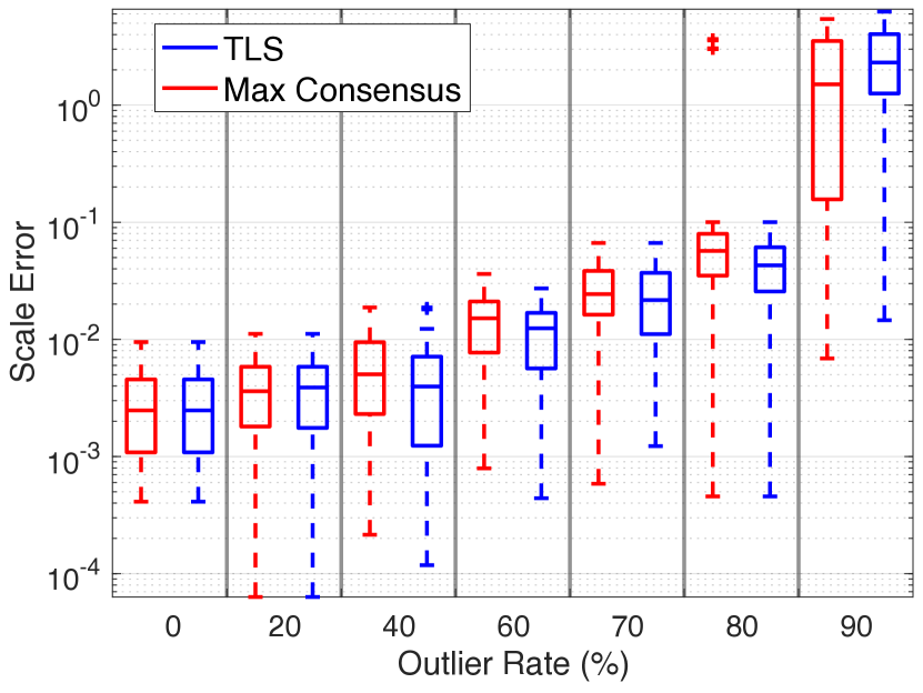
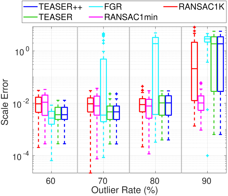
Scale Estimation. Given two point clouds and , we first create TIMs corresponding to a complete graph and then use Algorithm 2 to solve for the scale. We compute both Consensus Maximization [118] and TLS estimates of the scale. Fig. 4(a) shows box plots of the scale error with increasing outlier ratios. The scale error is computed as , where is the scale estimate and is the ground-truth. We observe the TLS solver is robust against 80% outliers, while Consensus Maximization failed twice in that regime.
 (a) Scale Estimation
|
 (b) MCIS
|
 (c) Rotation Estimation
|
 (d) Translation Estimation
|
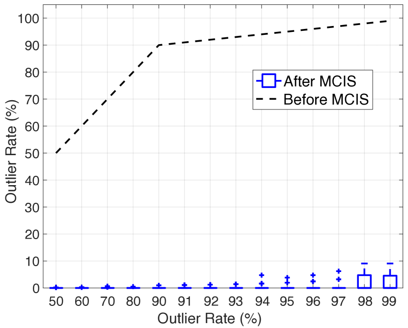
Maximal Clique Inlier Selection (MCIS). We downsample Bunny to and fix the scale to when applying the random transformation. We first prune the outlier TIMs/TRIMs (edges) that are not consistent with the scale , while keeping all the points (vertices), to obtain the graph . Then we compute the maximum clique in and remove all edges and vertices outside the maximum clique, obtaining a pruned graph (cf. line 1 in Algorithm 1). Fig. 4(b) shows the outlier ratio in (label: “Before MCIS”) and (label: “After MCIS”). MCIS effectively reduces outlier rate to below 10%, facilitating rotation and translation estimation, which, in isolation, can already tolerate more than 90% outliers ( when using GNC).
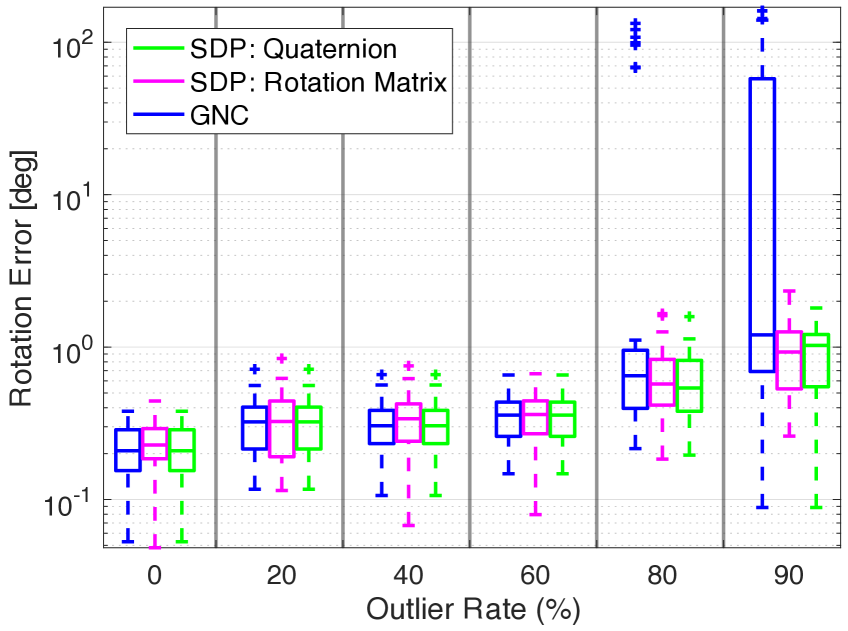
Rotation Estimation. We simulate TIMs by applying a random rotation to the Bunny, and fixing and (we set the number of TIMs to ). We compare three approaches to solve the TLS rotation estimation problem (14): (i) the quaternion-based SDP relaxation in eq. (29) and [39] (SDP: Quaternion), (ii) the rotation-matrix-based SDP relaxation we proposed in [38] (SDP: Rotation Matrix), and (iii) the GNC heuristic in [34]. For each approach, we evaluate the rotation error as , which is the geodesic distance between the rotation estimate (produced by each approach) and the ground-truth [119].
Fig. 4(c) reports the rotation error for increasing outlier rates. The GNC heuristic performs well below outliers and then starts failing. The two relaxations ensure similar performance, while the quaternion-based relaxation proposed in this paper is slightly more accurate at high outlier rates. Results in Appendix R show that the quaternion-based relaxation is always tighter than the relaxation in [38], which often translates into better estimates. The reader can find more experiments using our quaternion-based relaxation in [39], where we also demonstrate its robustness against over outliers and discuss applications to panorama stitching.
While the quaternion-based relaxation dominates in terms of accuracy and robustness, it requires solving a large SDP. Therefore, in TEASER++, we opted to use the fast GNC heuristic instead: this choice is motivated by the observation that MCIS is already able to remove most of the outliers (Fig. 4(b)) hence within TEASER++ the rotation estimation only requires solving a problem with less than 10% outliers.
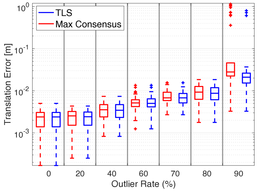
Translation Solver. We apply a random translation to the Bunny, and fix and . Fig. 4(d) shows that component-wise translation estimation using both Consensus Maximization and TLS are robust against 80% outliers. The translation error is defined as , the 2-norm of the difference between the estimate and the ground-truth . As mentioned above, most outliers are typically removed before translation estimation, hence enabling TEASER and TEASER++ to be robust to extreme outlier rates (more in Section XI-B).
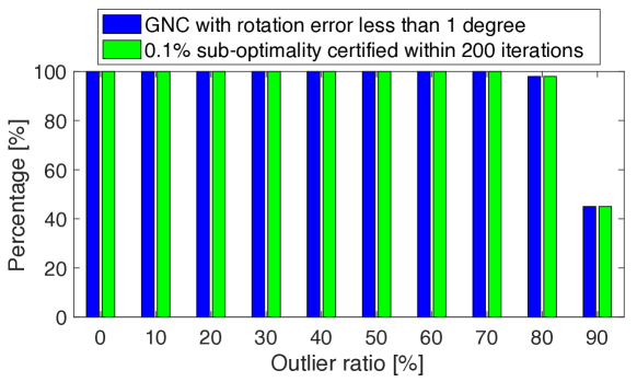
Optimality Certification for Rotation Estimation. We now test the effectiveness of Algorithm 3 in certifying optimality of a rotation estimate. We consider the same setup we used for testing rotation estimation but with TIMs. We use the GNC scheme in [34] to solve problem (14) and then use Algorithm 3 to certify the solution of GNC. Fig. 5 shows the performance of GNC and the certification algorithm under increasing outlier rates, where 100 Monte Carlo runs are performed at each outlier rate. The blue bars show the percentage of runs for which GNC produced a solution with less than 1 degree rotation error with respect to the ground truth; the green bars show the percentage of runs for which Algorithm 3 produced a relative sub-optimality bound lower than in less than 200 iterations of DRS. Fig. 5 demonstrates that: (i) the GNC scheme typically produces accurate solutions to the TLS rotation search problem with outliers (a result that confirms the errors we observed in Fig. 4(c)); (ii) the optimality certification algorithm 3 can certify all the correct GNC solutions and reject all incorrect GNC solutions within 200 iterations. On average, the certification algorithm takes iterations to obtain sub-optimality bound, where each DRS iteration takes 50ms in C++.
|

|
|
|
|
|
|
|
|
 (a) Known Scale
|
 (b) Known Scale (Extreme Outliers)
|
 (c) Unknown Scale
|
XI-B Benchmarking on Standard Datasets
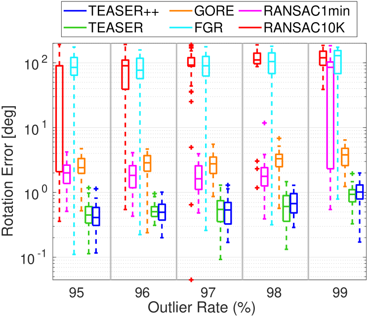
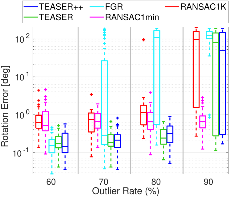
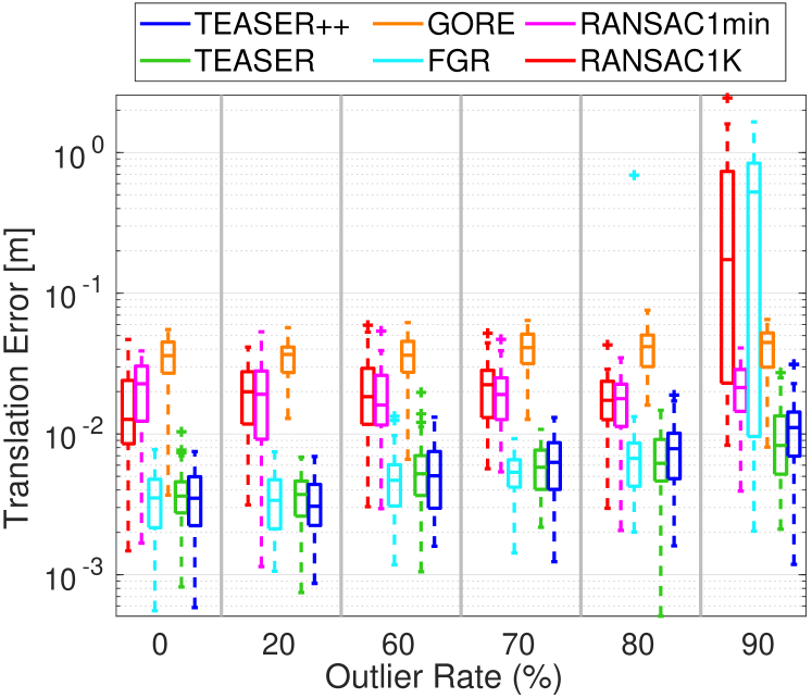
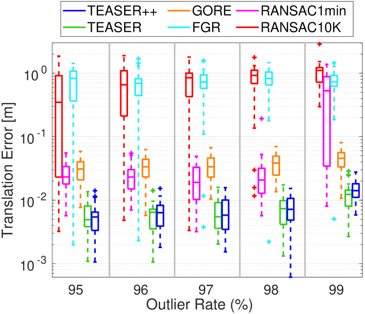
Testing Setup. We benchmark TEASER and TEASER++ against two state-of-the-art robust registration techniques: Fast Global Registration (FGR) [55] and Guaranteed Outlier REmoval (GORE) [19]. In addition, we test two RANSAC variants (with confidence): a fast version where we terminate RANSAC after a maximum of 1,000 iterations (RANSAC1K) and a slow version where we terminate RANSAC after 60 seconds (RANSAC1min). We use four datasets, Bunny, Armadillo, Dragon, and Buddha, from the Stanford 3D Scanning Repository [97] and downsample them to points. The tests below follow the same protocol of Section XI-A. Here we focus on the results on the Bunny dataset and we postpone the (qualitatively similar) results obtained on the other three datasets to Appendix S. Appendix S also showcases the proposed algorithms on registration problems with high noise (), and with up to 10,000 correspondences.
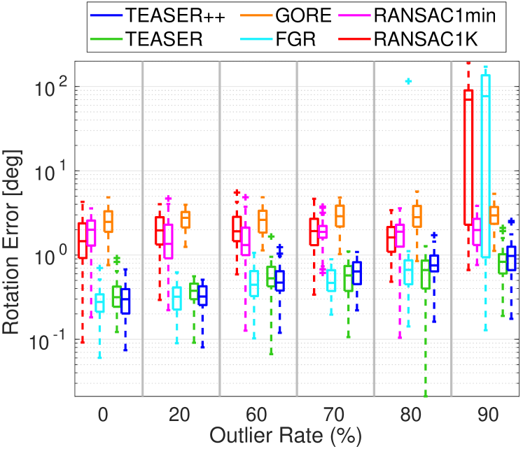
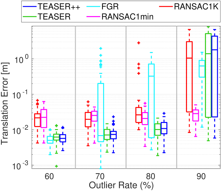
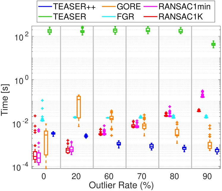
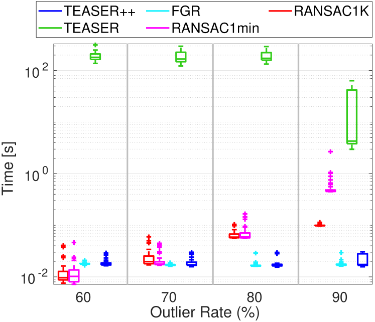
Known Scale. We first evaluate the compared techniques with known scale . Fig. 6(a) shows the rotation error, translation error, and timing for increasing outlier rates on the Bunny dataset. From the rotation and translation errors, we note that TEASER, TEASER++, GORE, and RANSAC1min are robust against up to 90% outliers, although TEASER and TEASER++ tend to produce more accurate estimates than GORE, and RANSAC1min typically requires over iterations for convergence at 90% outlier rate. FGR can only resist 70% outliers and RANSAC1K starts breaking at 90% outliers. TEASER++’s performance is on par with TEASER for all outlier rates, which is expected from the observations in Section X. The timing subplot at the bottom of Fig. 6(a) shows that TEASER is impractical for real-time robotics applications. On the other hand, TEASER++ is one of the fastest techniques across the spectrum, and is able to solve problems with large number of outliers in less than 10ms on a standard laptop.
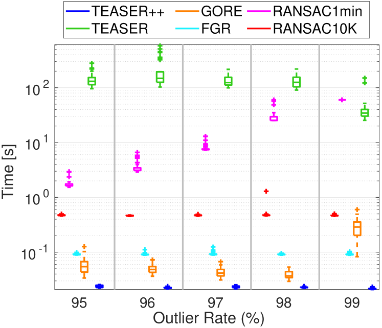
Extreme Outlier Rates. We further benchmark the performance of TEASER and TEASER++ under extreme outlier rates from 95% to 99% with known scale and correspondences on the Bunny. We replace RANSAC1K with RANSAC10K, since RANSAC1K already performs poorly at 90% outliers. Fig. 6(b) shows the boxplots of the rotation errors, translation errors, and timing. TEASER, TEASER++, and GORE are robust against up to 99% outliers, while RANSAC1min with 60s timeout can resist 98% outliers with about iterations. RANSAC10K and FGR perform poorly under extreme outlier rates. While GORE, TEASER and TEASER++ are both robust against 99% outliers, TEASER, and TEASER++ produce lower estimation errors, with TEASER++ being one order of magnitude faster than GORE (bottom subfigure). We remark that TEASER++’s robustness against outliers is due in large part to the drastic reduction of outlier rates by MCIS.
Unknown Scale. GORE is unable to solve for the scale, hence we only benchmark TEASER and TEASER++ against FGR,888Although the original algorithm in [55] did not solve for the scale, we extend it by using Horn’s method to compute the scale at each iteration RANSAC1K, and RANSAC1min. Fig. 6(c) plots scale, rotation, translation error and timing for increasing outliers on the Bunny dataset. All the compared techniques perform well when the outlier ratio is below 60%. FGR has the lowest breakdown point and fails at 70%. RANSAC1K, TEASER, and TEASER++ only fail at 90% outlier ratio when the scale is unknown. Although RANSAC1min with 60s timeout outperforms other methods at 90% outliers, it typically requires more than iterations to converge, which is not practical for real-time applications. TEASER++ consistently runs in less than 30ms.
XI-C Simultaneous Pose and Correspondences (SPC)
Here we provide a proof-of-concept of how to use TEASER++ in the case where we do not have correspondences.
Testing Setup. We obtain the source point cloud by downsampling the Bunny dataset to points. Then, we create the point cloud by applying a random rotation and translation to . Finally. we remove a percentage of the points in to simulate partial overlap between and . For instance, when the overlap is , we discard (randomly chosen) points from . We compare TEASER++ against (i) ICP initialized with the identity transformation; and (ii) Go-ICP [20] with , and trimming percentages to be robust to partial overlap. For TEASER++, we generate all possible correspondences: in other words, for each point in we add all points in as a potential correspondence (for a total of correspondences). We then feed the correspondences to TEASER++ that computes a transformation without the need for an initial guess. Clearly, most of the correspondences fed to TEASER are outliers, but we rely on TEASER++ to find the small set of inliers.
Fig. 7(a)-(b) show the rotation and translation errors for different levels of overlap between and . ICP fails to compute the correct transformation in practically all instances, since the initial guess is not in the basin of convergence of the optimal solution. Go-ICP is a global method which does not require an initial guess and performs much better than ICP. However, Go-ICP requires the user to set a trimming percentage to deal with partial overlap, and Fig. 7(a)-(b) show the performance of Go-ICP is highly sensitive to the trimming percentage (Go-ICP () performs the best but is still less accurate than TEASER++). Moreover, Go-ICP takes 16 seconds on average due to its usage of BnB. TEASER++ computes a correct solution across the spectrum without the need for an initial guess. TEASER++ only starts failing when the overlap drops below . The price we pay for this enhanced robustness is an increase in runtime. We feed correspondences to TEASER++, which increases the runtime compared to the correspondence-based setup in which the number of correspondences scales linearly (rather than quadratically) with the point cloud size. Fig. 7(c) reports the timing breakdown for the different modules in TEASER++. From the figure, we observe that (i) for small overlap, TEASER++ is not far from real-time, (ii) the timing is dominated by the maximum clique computation and scale estimation, where the latter includes the computation of the translation and rotation invariant measurements (TRIMs), and (iii) TEASER++ is orders of magnitude faster than Go-ICP when the overlap is low (e.g., below ).
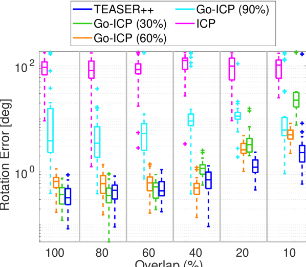 (a) Rotation Error
|
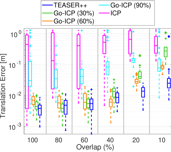 (b) Translation Error
|
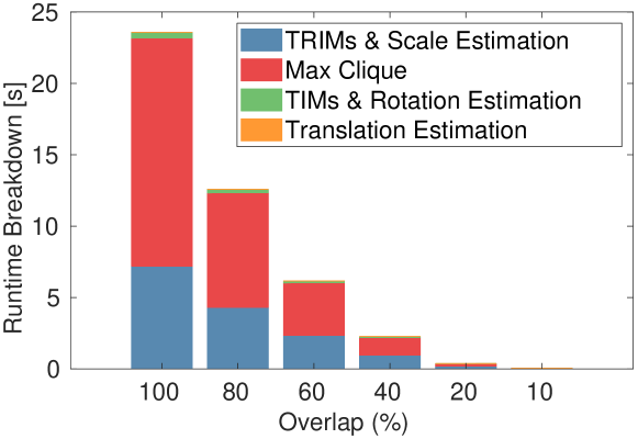 (c) Timing Breakdown
|
|
|
| Mean | SD | |
| Rotation error [rad] | 0.066 | 0.043 |
| Translation error [m] | 0.069 | 0.053 |
| # of FPFH correspondences | 525 | 161 |
| FPFH inlier ratio [%] | 6.53 | 4.59 |
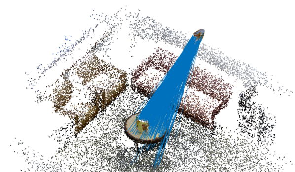
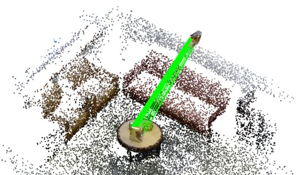
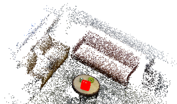
XI-D Application 1: Object Pose Estimation and Localization
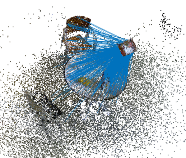
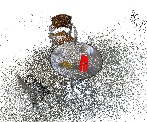
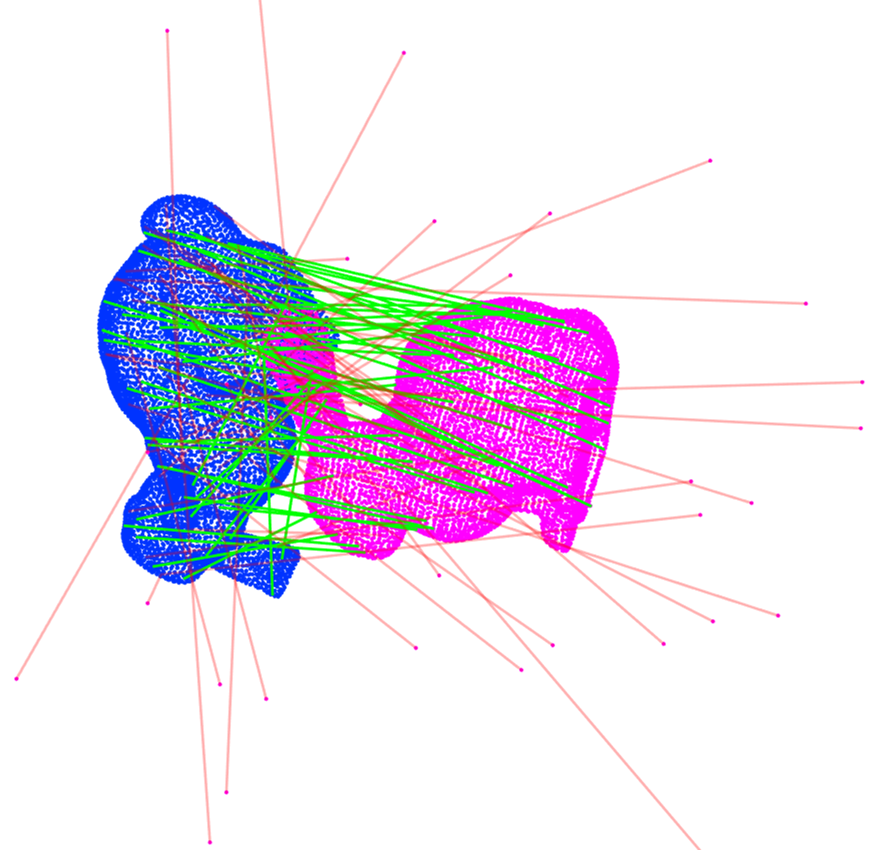
Testing Setup. We use the large-scale point cloud datasets from [36] to test TEASER in object pose estimation and localization applications. We first use the ground-truth object labels to extract the cereal box/cap out of the scene and treat it as the object, then apply a random transformation to the scene, to get an object-scene pair. To register the object-scene pair, we first use FPFH feature descriptors [1] to establish putative correspondences. Given correspondences from FPFH, TEASER is used to find the relative pose between the object and scene. We downsample the object and scene using the same ratio (about 0.1) to make the object have 2,000 points.
Results. Fig. 8 shows the noisy FPFH correspondences, the inlier correspondences obtained by TEASER, and successful localization and pose estimation of the cereal box. Another example is given in Fig. 1(g)-(h). Qualitative results for eight scenes are given in Appendix T. The inlier correspondence ratios for cereal box are all below 10% and typically below 5%. TEASER is able to compute a highly accurate estimate of the pose using a handful of inliers. Table 8 shows the mean and standard deviation (SD) of the rotation and translation errors, the number of FPFH correspondences, and the inlier ratio estimated by TEASER on the eight scenes.
XI-E Application 2: Scan Matching
Testing Setup. TEASER++ can also be used in robotics applications that need robust scan matching, such as 3D reconstruction and loop closure detection in SLAM [120]. We evaluate TEASER++’s performance in such scenarios using the 3DMatch dataset [37], which consists of RGB-D scans from 62 real-world indoor scenes. The dataset is divided into 54 scenes for training, and 8 scenes for testing. The authors provide 5,000 randomly sampled keypoints for each scan. On average, there are 205 pairs of scans per scene (maximum: 519 in the Kitchen scene, minimum: 54 in the Hotel 3 scene).
|
| Scenes | |||||||||
|---|---|---|---|---|---|---|---|---|---|
|
Kitchen (%)
|
Home 1 (%)
|
Home 2 (%)
|
Hotel 1 (%)
|
Hotel 2 (%)
|
Hotel 3 (%)
|
Study (%)
|
MIT Lab (%)
|
Avg. Runtime [s]
|
|
| RANSAC-1K | 91.3 | 89.1 | 74.5 | 94.2 | 84.6 | 90.7 | 86.3 | 81.8 | 0.008 |
| RANSAC-10K | 97.2 | 92.3 | 79.3 | 96.5 | 86.5 | 94.4 | 90.4 | 85.7 | 0.074 |
| TEASER++ | 98.6 | 92.9 | 86.5 | 97.8 | 89.4 | 94.4 | 91.1 | 83.1 | 0.059 |
| TEASER++ (CERT) | 99.4 | 94.1 | 88.7 | 98.2 | 91.9 | 94.4 | 94.3 | 88.6 | 238.136 |
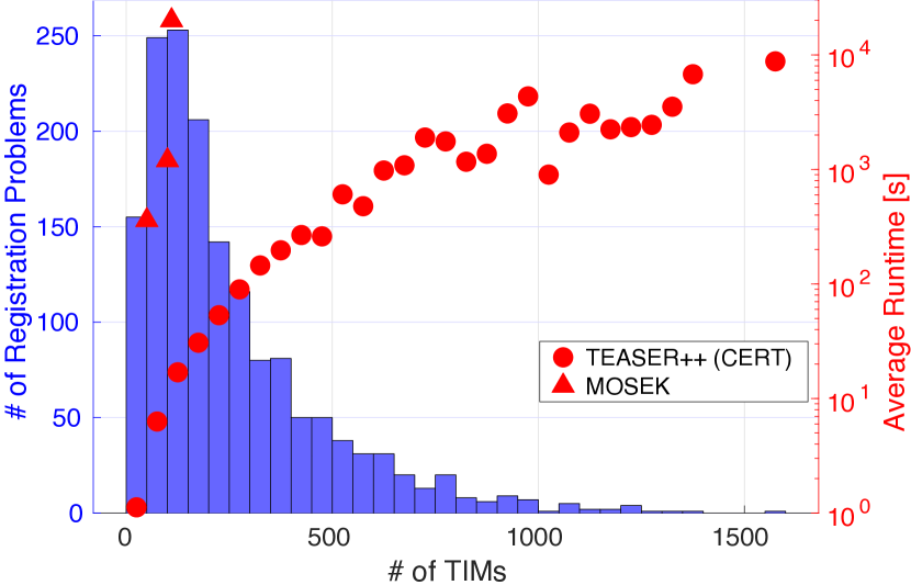
We use 3DSmoothNet [2], a state-of-the-art neural network, to compute local descriptors for each 3D keypoint, and generate correspondences using nearest-neighbor search. We then feed the correspondences to TEASER++ and RANSAC (implemented in Open3D [121]) and compare their performance in terms of percentage of successfully matched scans and runtime. Due to the large number of pairs we need to test, we run the experiments on a server with a Xeon Platinum 8259CL CPU at 2.50GHz, and allocate 12 threads for each algorithm under test. Two scans are successful matched when the transformation computed by a technique has (i) rotation error smaller than , and (ii) translation error less than . We report RANSAC’s results with maximum number of iterations equal to 1,000 (RANSAC1K) and 10,000 (RANSAC10K). We also compare the percentage of successful registrations out of the cases where TEASER++ certified the rotation estimation as optimal, a setup we refer to as TEASER++ (CERT). The latter executes Algorithm 3 to evaluate the poses from TEASER++ and uses a desired sub-optimality gap to certify optimality. We use for TEASER++ in all tests.
Results. Table 9 shows the percentage of successfully matched scans and the average timing for the four compared techniques. TEASER dominates both RANSAC variants with exception of the Lab scene. RANSAC1K has a success rate up to worst than TEASER++. RANSAC10K is an optimized C++ implementation and, while running slower than TEASER++, it cannot reach the same accuracy for most scenes. These results further highlight that TEASER++ can be safely used as a faster and more robust replacement for RANSAC in SLAM pipelines. This conclusion is further reinforced by the last row in Table 9, where we show the success rate for the poses certified as optimal by TEASER++. The success rate strictly dominates both RANSAC variants and TEASER++, since TEASER++ (CERT) is able to identify and reject unreliable registration results. This is a useful feature when scan matching is used for loop closure detection in SLAM, since bad registration results lead to incorrect loop closures and can compromise the quality of the resulting map (see [54, 34]). While running Algorithm 3 in TEASER++ (CERT) requires more than 200 seconds in average, the majority of instances are solved by TEASER++ (CERT) within 100 seconds and problems with fewer than 50 TIMs can be certified in 1.12 seconds. Fig. 9 compares the runtime of our certification approach against MOSEK (which directly solves the SDP relaxation) for 50, 100, and 110 TIMs. We can see that TEASER++ (CERT) is orders of magnitude faster, and can certify large-scale problems beyond the reach of MOSEK, which runs out of memory for over 150 TIMs.
Why is TEASER++ not able to solve 100% of the tests in Table 9? This should not come as a surprise from the statements in Theorem 15-17. The estimation contracts discussed in Section IX require a minimum number of inliers: TEASER++ can mine a small number of inliers among a large number of outliers, but it cannot solve problems where no inliers are given or where the inliers are not enough to identify a unique registration! For the experiments in this section, it is not uncommon to have no or fewer than 3 inliers in a scene due to the quality of the keypoint descriptors. Moreover, it is not uncommon to have symmetries in the scene, which make the registration non-unique. To intuitively highlight this issue, Fig. 10 shows the rotation errors of TEASER++, with different markers for certified (blue dots) and non-certified (red crosses) solutions. The figure shows that (i) TEASER++ (CERT) is able to reject a large number of incorrect estimates (red crosses with large errors), and (ii) some of the incorrect but certified solutions exhibit errors around and which correspond to symmetries of the scene. A visual example of the phenomenon is shown in Fig. 11. These results highlight the need for better keypoint detectors, since even state-of-the-art deep-learning-based methods struggle to produce acceptable outlier rates in real problems.
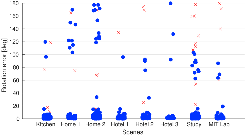
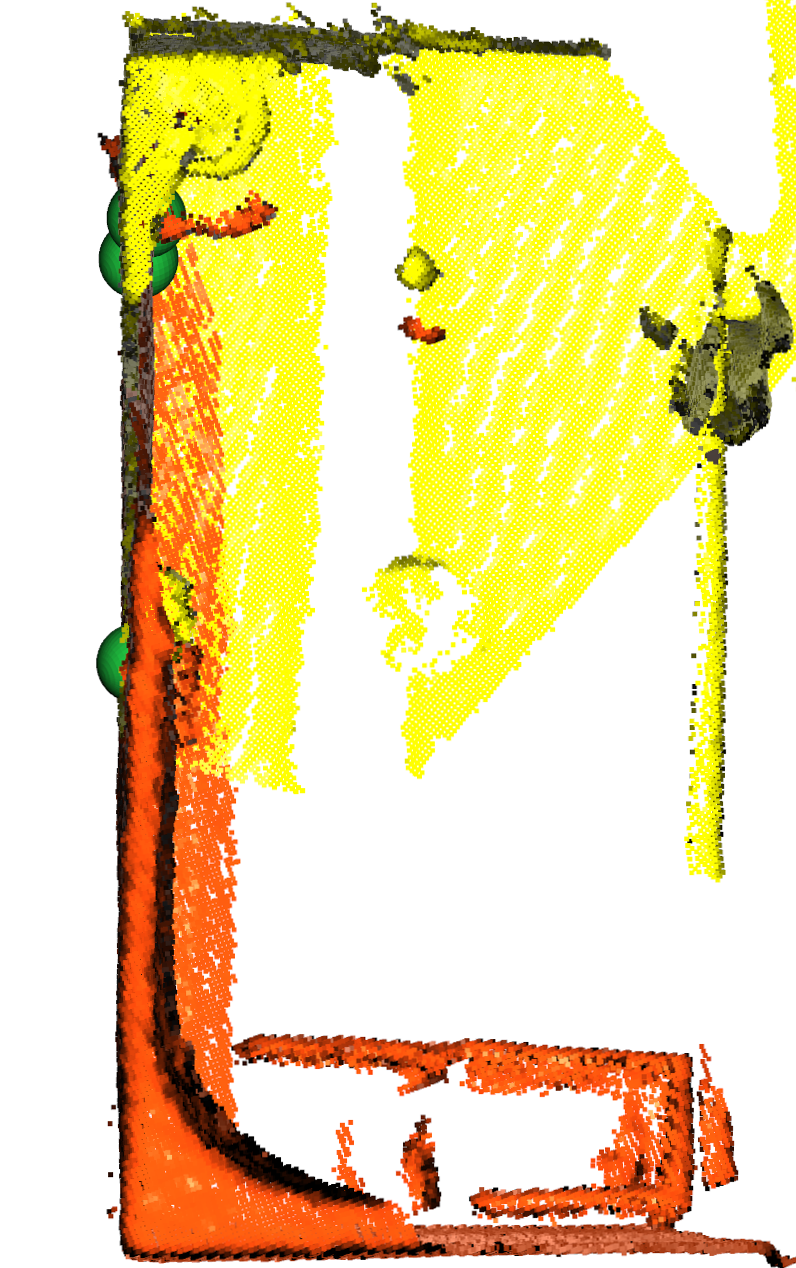 (a) Ground truth
(top-down view)
(a) Ground truth
(top-down view)
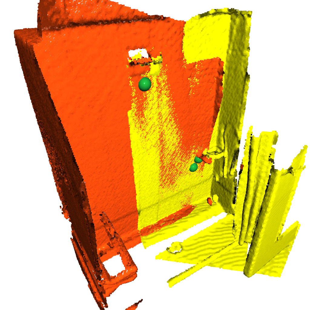 |
| (b) Ground truth |
| (side view) |
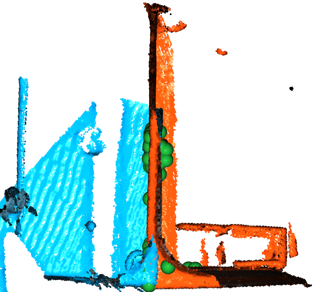 |
| (c) TEASER++’s estimate |
| (top-down view) |
XII Conclusion
We propose the first fast and certifiable algorithm for correspondence-based registration with extreme outlier rates. We leverage insights from estimation theory (e.g., unknown-but-bounded noise), geometry (e.g., invariant measurements), graph theory (e.g., maximum clique for inlier selection), and optimization (e.g., tight SDP relaxations). These insights lead to the design of two certifiable registration algorithms. TEASER is accurate and robust but requires solving a large SDP. TEASER++ has similar performance in practice but circumvents the need to solve an SPD and can run in milliseconds. TEASER++ is also certifiable by leveraging Douglas-Rachford Splitting to compute a dual optimality certificate. For both algorithms, we provide theoretical bounds on the estimation errors, which are the first of their kind for robust registration problems. Moreover, we test their performance on standard benchmarks, object detection datasets, and the 3DMatch scan matching dataset and show that (i) both algorithms dominate the state of the art (e.g., RANSAC, BnB, heuristics) and are robust to more than outliers, (ii) TEASER++ can run in milliseconds and it is currently the fastest robust registration algorithm at high outlier rates, (iii) TEASER++ is so robust it can also solve problems without correspondences (e.g., hypothesizing all-to-all correspondences) where it outperforms ICP and Go-ICP. We release a fast open-source C++ implementation of TEASER++.
While not central to the technical contribution, this paper also establishes the foundations of certifiable perception, as discussed in Appendix A. This research area offers many research opportunities and the resulting progress has the potential to boost trustworthiness and reliability in safety-critical application of robotics and computer vision. Future work includes developing certifiable algorithms for other spatial perception problems (ideally leading to certifiable approaches for all the applications discussed in [34] and more). Another avenue for future research is the use of the certifiably robust algorithms presented in this paper for self-supervision of deep learning methods for keypoint detection and matching.
References
- [1] R. Rusu, N. Blodow, and M. Beetz, “Fast point feature histograms (fpfh) for 3d registration,” in IEEE Intl. Conf. on Robotics and Automation (ICRA). Citeseer, 2009, pp. 3212–3217.
- [2] Z. Gojcic, C. Zhou, J. D. Wegner, and A. Wieser, “The perfect match: 3d point cloud matching with smoothed densities,” in Proceedings of the IEEE Conference on Computer Vision and Pattern Recognition, 2019, pp. 5545–5554.
- [3] P. Henry, M. Krainin, E. Herbst, X. Ren, and D. Fox, “Rgb-d mapping: Using kinect-style depth cameras for dense 3d modeling of indoor environments,” Intl. J. of Robotics Research, vol. 31, no. 5, pp. 647–663, 2012.
- [4] G. Blais and M. D. Levine, “Registering multiview range data to create 3d computer objects,” IEEE Trans. Pattern Anal. Machine Intell., vol. 17, no. 8, pp. 820–824, 1995.
- [5] S. Choi, Q. Y. Zhou, and V. Koltun, “Robust reconstruction of indoor scenes,” in IEEE Conf. on Computer Vision and Pattern Recognition (CVPR), 2015, pp. 5556–5565.
- [6] J. Zhang and S. Singh, “Visual-lidar odometry and mapping: Low-drift, robust, and fast,” in IEEE Intl. Conf. on Robotics and Automation (ICRA). IEEE, 2015, pp. 2174–2181.
- [7] B. Drost, M. Ulrich, N. Navab, and S. Ilic, “Model globally, match locally: Efficient and robust 3D object recognition,” in IEEE Conf. on Computer Vision and Pattern Recognition (CVPR), 2010, pp. 998–1005.
- [8] J. M. Wong, V. Kee, T. Le, S. Wagner, G. L. Mariottini, A. Schneider, L. Hamilton, R. Chipalkatty, M. Hebert, D. M. S. Johnson et al., “Segicp: Integrated deep semantic segmentation and pose estimation,” in IEEE/RSJ Intl. Conf. on Intelligent Robots and Systems (IROS). IEEE, 2017, pp. 5784–5789.
- [9] A. Zeng, K. T. Yu, S. Song, D. Suo, E. Walker, A. Rodriguez, and J. Xiao, “Multi-view self-supervised deep learning for 6d pose estimation in the amazon picking challenge,” in IEEE Intl. Conf. on Robotics and Automation (ICRA). IEEE, 2017, pp. 1386–1383.
- [10] P. Marion, P. R. Florence, L. Manuelli, and R. Tedrake, “Label fusion: A pipeline for generating ground truth labels for real rgbd data of cluttered scenes,” in IEEE Intl. Conf. on Robotics and Automation (ICRA). IEEE, 2018, pp. 1–8.
- [11] J. Bazin, Y. Seo, R. Hartley, and M. Pollefeys, “Globally optimal inlier set maximization with unknown rotation and focal length,” in European Conf. on Computer Vision (ECCV), 2014, pp. 803–817.
- [12] M. A. Audette, F. P. Ferrie, and T. M. Peters, “An algorithmic overview of surface registration techniques for medical imaging,” Med. Image Anal., vol. 4, no. 3, pp. 201–217, 2000.
- [13] G. K. L. Tam, Z. Q. Cheng, Y. K. Lai, F. C. Langbein, Y. Liu, D. Marshall, R. R. Martin, X. F. Sun, and P. L. Rosin, “Registration of 3d point clouds and meshes: a survey from rigid to nonrigid.” IEEE Trans. Vis. Comput. Graph., vol. 19, no. 7, pp. 1199–1217, 2013.
- [14] B. K. P. Horn, “Closed-form solution of absolute orientation using unit quaternions,” J. Opt. Soc. Amer., vol. 4, no. 4, pp. 629–642, Apr 1987.
- [15] K. Arun, T. Huang, and S. Blostein, “Least-squares fitting of two 3-D point sets,” IEEE Trans. Pattern Anal. Machine Intell., vol. 9, no. 5, pp. 698–700, sept. 1987.
- [16] F. Tombari, S. Salti, and L. D. Stefano, “Performance evaluation of 3d keypoint detectors,” Intl. J. of Computer Vision, vol. 102, no. 1-3, pp. 198–220, 2013.
- [17] P. J. Besl and N. D. McKay, “A method for registration of 3-D shapes,” IEEE Trans. Pattern Anal. Machine Intell., vol. 14, no. 2, 1992.
- [18] M. Fischler and R. Bolles, “Random sample consensus: a paradigm for model fitting with application to image analysis and automated cartography,” Commun. ACM, vol. 24, pp. 381–395, 1981.
- [19] Á. Parra Bustos and T. J. Chin, “Guaranteed outlier removal for point cloud registration with correspondences,” IEEE Trans. Pattern Anal. Machine Intell., vol. 40, no. 12, pp. 2868–2882, 2018.
- [20] J. Yang, H. Li, D. Campbell, and Y. Jia, “Go-ICP: A globally optimal solution to 3D ICP point-set registration,” IEEE Trans. Pattern Anal. Machine Intell., vol. 38, no. 11, pp. 2241–2254, Nov. 2016.
- [21] A. Bandeira, “A note on probably certifiably correct algorithms,” Comptes Rendus Mathematique, vol. 354, no. 3, pp. 329–333, 2016.
- [22] L. Carlone and F. Dellaert, “Duality-based verification techniques for 2D SLAM,” in IEEE Intl. Conf. on Robotics and Automation (ICRA), 2015, pp. 4589–4596, (pdf) (code).
- [23] D. Rosen, L. Carlone, A. Bandeira, and J. Leonard, “SE-Sync: a certifiably correct algorithm for synchronization over the Special Euclidean group,” Intl. J. of Robotics Research, 2018, accepted, arxiv preprint: 1611.00128, (pdf).
- [24] Q. M. Rahman, N. Sünderhauf, and F. Dayoub, “Did you miss the sign? A false negative alarm system for traffic sign detectors,” CoRR, vol. abs/1903.06391, 2019. [Online]. Available: http://arxiv.org/abs/1903.06391
- [25] S. Seshia and D. Sadigh, “Towards verified artificial intelligence,” ArXiv, vol. abs/1606.08514, 2016.
- [26] A. Desai, T. Dreossi, and S. Seshia, “Combining model checking and runtime verification for safe robotics,” in International Conference on Runtime Verification. Springer, 2017, pp. 172–189.
- [27] A. Makadia, A. Patterson, and K. Daniilidis, “Fully automatic registration of 3d point clouds,” in IEEE Conf. on Computer Vision and Pattern Recognition (CVPR), vol. 1, 2006, pp. 1297–1304.
- [28] Y. Liu, C. Wang, Z. Song, and M. Wang, “Efficient global point cloud registration by matching rotation invariant features through translation search,” in European Conf. on Computer Vision (ECCV), September 2018.
- [29] M. Milanese, Estimation and Prediction in the Presence of Unknown but Bounded Uncertainty: A Survey. Boston, MA: Springer US, 1989, pp. 3–24.
- [30] D. Bertsekas, “Control of uncertain systems with a set-membership description of the uncertainty,” Ph.D. dissertation, Massachusetts Institute of Technology, 1971.
- [31] R. Hartley and F. Kahl, “Global optimization through rotation space search,” Intl. J. of Computer Vision, vol. 82, no. 1, pp. 64–79, 2009.
- [32] G. Wahba, “A least squares estimate of satellite attitude,” SIAM review, vol. 7, no. 3, pp. 409–409, 1965.
- [33] I. Diakonikolas, G. Kamath, D. Kane, J. Li, A. Moitra, and A. Stewart, “Robust estimators in high dimensions without the computational intractability,” in IEEE 57th Annual Symposium on Foundations of Computer Science. IEEE, 2016, pp. 655–664.
- [34] H. Yang, P. Antonante, V. Tzoumas, and L. Carlone, “Graduated non-convexity for robust spatial perception: From non-minimal solvers to global outlier rejection,” IEEE Robotics and Automation Letters (RA-L), vol. 5, no. 2, pp. 1127–1134, 2020, arXiv preprint arXiv:1909.08605 (with supplemental material), (pdf).
- [35] H. Yang and L. Carlone, “One ring to rule them all: Certifiably robust geometric perception with outliers,” in Advances in Neural Information Processing Systems (NIPS), 2020.
- [36] K. Lai, L. Bo, X. Ren, and D. Fox, “A large-scale hierarchical multi-view RGB-D object dataset,” in IEEE Intl. Conf. on Robotics and Automation (ICRA). IEEE, 2011, pp. 1817–1824.
- [37] A. Zeng, S. Song, M. Nießner, M. Fisher, J. Xiao, and T. Funkhouser, “3dmatch: Learning the matching of local 3d geometry in range scans,” in Proceedings of the IEEE Conference on Computer Vision and Pattern Recognition, vol. 1, no. 2, 2017, p. 4.
- [38] H. Yang and L. Carlone, “A polynomial-time solution for robust registration with extreme outlier rates,” in Robotics: Science and Systems (RSS), 2019, (pdf), (video), (media), (media), (media).
- [39] ——, “A quaternion-based certifiably optimal solution to the Wahba problem with outliers,” in Intl. Conf. on Computer Vision (ICCV), 2019, (Oral Presentation, accept rate: 4%), Arxiv version: 1905.12536, (pdf).
- [40] C. Choy, J. Park, and V. Koltun, “Fully convolutional geometric features,” in Intl. Conf. on Computer Vision (ICCV), 2019, pp. 8958–8966.
- [41] C. Olsson, F. Kahl, and M. Oskarsson, “Branch-and-bound methods for euclidean registration problems,” IEEE Trans. Pattern Anal. Machine Intell., vol. 31, no. 5, pp. 783–794, 2009.
- [42] J. Briales and J. Gonzalez-Jimenez, “Convex Global 3D Registration with Lagrangian Duality,” in IEEE Conf. on Computer Vision and Pattern Recognition (CVPR), 2017.
- [43] F. L. Markley and J. L. Crassidis, Fundamentals of spacecraft attitude determination and control. Springer, 2014, vol. 33.
- [44] F. L. Markley, “Attitude determination using vector observations and the singular value decomposition,” The Journal of the Astronautical Sciences, vol. 36, no. 3, pp. 245–258, 1988.
- [45] J. Gower and G. Dijksterhuis, “Procrustes problems,” Procrustes Problems, Oxford Statistical Science Series, vol. 30, 01 2005.
- [46] P. Schonemann, “A generalized solution of the orthogonal procrustes problem,” Psychometrika, vol. 31, pp. 1–10, 1966.
- [47] N. Ohta and K. Kanatani, “Optimal estimation of three-dimensional rotation and reliability evaluation,” IEICE TRANSACTIONS on Information and Systems, vol. 81, no. 11, pp. 1247–1252, 1998.
- [48] Y. Cheng and J. L. Crassidis, “A total least-squares estimate for attitude determination,” in AIAA Scitech 2019 Forum, 2019, p. 1176.
- [49] S. Ahmed, E. C. Kerrigan, and I. M. Jaimoukha, “A semidefinite relaxation-based algorithm for robust attitude estimation,” IEEE Transactions on Signal Processing, vol. 60, no. 8, pp. 3942–3952, 2012.
- [50] R. Hartley and A. Zisserman, Multiple View Geometry in Computer Vision. Cambridge University Press, 2000.
- [51] P. Meer, D. Mintz, A. Rosenfeld, and D. Y. Kim, “Robust regression methods for computer vision: A review,” Intl. J. of Computer Vision, vol. 6, no. 1, pp. 59–70, Apr 1991.
- [52] K. M. Tavish and T. D. Barfoot, “At all costs: A comparison of robust cost functions for camera correspondence outliers,” in Computer and Robot Vision (CRV), 2015 12th Conference on. IEEE, 2015, pp. 62–69.
- [53] M. J. Black and A. Rangarajan, “On the unification of line processes, outlier rejection, and robust statistics with applications in early vision,” Intl. J. of Computer Vision, vol. 19, no. 1, pp. 57–91, 1996.
- [54] P. Lajoie, S. Hu, G. Beltrame, and L. Carlone, “Modeling perceptual aliasing in SLAM via discrete-continuous graphical models,” IEEE Robotics and Automation Letters (RA-L), 2019, extended ArXiv version: (pdf), Supplemental Material: (pdf).
- [55] Q. Zhou, J. Park, and V. Koltun, “Fast global registration,” in European Conf. on Computer Vision (ECCV). Springer, 2016, pp. 766–782.
- [56] O. Enqvist, K. Josephson, and F. Kahl, “Optimal correspondences from pairwise constraints,” in Intl. Conf. on Computer Vision (ICCV), 2009, pp. 1295–1302.
- [57] A. Parra Bustos, T.-J. Chin, F. Neumann, T. Friedrich, and M. Katzmann, “A practical maximum clique algorithm for matching with pairwise constraints,” arXiv preprint arXiv:1902.01534, 2019.
- [58] V. Golyanik, S. Aziz Ali, and D. Stricker, “Gravitational approach for point set registration,” in IEEE Conf. on Computer Vision and Pattern Recognition (CVPR), 2016, pp. 5802–5810.
- [59] P. Jauer, I. Kuhlemann, R. Bruder, A. Schweikard, and F. Ernst, “Efficient registration of high-resolution feature enhanced point clouds,” IEEE Trans. Pattern Anal. Machine Intell., vol. 41, no. 5, pp. 1102–1115, 2018.
- [60] H. Yang, “A dynamical perspective on point cloud registration,” arXiv preprint arXiv:2005.03190, 2020.
- [61] T. J. Chin and D. Suter, “The maximum consensus problem: recent algorithmic advances,” Synthesis Lectures on Computer Vision, vol. 7, no. 2, pp. 1–194, 2017.
- [62] F. Wen, R. Ying, Z. Gong, and P. Liu, “Efficient algorithms for maximum consensus robust fitting,” IEEE Trans. Robotics, 2019.
- [63] Z. Cai, T.-J. Chin, and V. Koltun, “Consensus maximization tree search revisited,” in Intl. Conf. on Computer Vision (ICCV), 2019, pp. 1637–1645.
- [64] H. M. Le, T.-J. Chin, A. Eriksson, T.-T. Do, and D. Suter, “Deterministic approximate methods for maximum consensus robust fitting,” IEEE Trans. Pattern Anal. Machine Intell., 2019.
- [65] V. Tzoumas, P. Antonante, and L. Carlone, “Outlier-robust spatial perception: Hardness, general-purpose algorithms, and guarantees,” in IEEE/RSJ Intl. Conf. on Intelligent Robots and Systems (IROS), 2019, extended arxiv version: 1903.11683, (pdf).
- [66] T.-J. Chin, Z. Cai, and F. Neumann, “Robust fitting in computer vision: Easy or hard?” in European Conf. on Computer Vision (ECCV), 2018.
- [67] D. Campbell, L. Petersson, L. Kneip, and H. Li, “Globally-optimal inlier set maximisation for simultaneous camera pose and feature correspondence,” in Intl. Conf. on Computer Vision (ICCV), 2017, pp. 1–10.
- [68] J. C. Bazin, Y. Seo, and M. Pollefeys, “Globally optimal consensus set maximization through rotation search,” in Asian Conference on Computer Vision. Springer, 2012, pp. 539–551.
- [69] C. Olsson, O. Enqvist, and F. Kahl, “A polynomial-time bound for matching and registration with outliers,” in IEEE Conf. on Computer Vision and Pattern Recognition (CVPR). IEEE, 2008, pp. 1–8.
- [70] O. Enqvist, E. Ask, F. Kahl, and K. Åström, “Robust fitting for multiple view geometry,” in European Conf. on Computer Vision (ECCV). Springer, 2012, pp. 738–751.
- [71] E. Ask, O. Enqvist, and F. Kahl, “Optimal geometric fitting under the truncated -norm,” in IEEE Conf. on Computer Vision and Pattern Recognition (CVPR), 2013, pp. 1722–1729.
- [72] S. Granger and X. Pennec, “Multi-scale EM-ICP: A fast and robust approach for surface registration,” in European Conf. on Computer Vision (ECCV), 2002.
- [73] L. Maier-Hein, A. M. Franz, T. R. dos Santos, M. Schmidt, M. Fangerau, H. P. Meinzer, and J. M. Fitzpatrick, “Convergent iterative closest-point algorithm to accomodate anisotropic and inhomogenous localization error,” IEEE Trans. Pattern Anal. Machine Intell., vol. 34, no. 8, pp. 1520–1532, 2012.
- [74] D. Chetverikov, D. Stepanov, and P. Krsek, “Robust euclidean alignment of 3D point sets: the trimmed iterative closest point algorithm,” Image and Vision Computing, vol. 23, no. 3, pp. 299–309, 2005.
- [75] S. Kaneko, T. Kondo, and A. Miyamoto, “Robust matching of 3D contours using iterative closest point algorithm improved by M-estimation,” Pattern Recognition, vol. 36, no. 9, pp. 2041–2047, 2003.
- [76] A. Myronenko and X. Song, “Point set registration: Coherent point drift,” IEEE Trans. Pattern Anal. Machine Intell., vol. 32, no. 12, pp. 2262–2275, 2010.
- [77] B. Jian and B. C. Vemuri, “Robust point set registration using gaussian mixture models,” IEEE Trans. Pattern Anal. Machine Intell., vol. 33, no. 8, pp. 1633–1645, 2011.
- [78] W. Clark, M. Ghaffari, and A. Bloch, “Nonparametric continuous sensor registration,” arXiv preprint arXiv:2001.04286, 2020.
- [79] H. M. Le, T.-T. Do, T. Hoang, and N.-M. Cheung, “SDRSAC: Semidefinite-based randomized approach for robust point cloud registration without correspondences,” in IEEE Conf. on Computer Vision and Pattern Recognition (CVPR), 2019, pp. 124–133.
- [80] T. M. Breuel, “Implementation techniques for geometric branch-and-bound matching methods,” Comput. Vis. Image Underst., vol. 90, no. 3, pp. 258–294, 2003.
- [81] Á. Parra Bustos, T. J. Chin, and D. Suter, “Fast rotation search with stereographic projections for 3d registration,” in IEEE Conf. on Computer Vision and Pattern Recognition (CVPR), 2014, pp. 3930–3937.
- [82] H. Li and R. Hartley, “The 3D-3D registration problem revisited,” in Intl. Conf. on Computer Vision (ICCV). IEEE, 2007, pp. 1–8.
- [83] G. Izatt, H. Dai, and R. Tedrake, “Globally optimal object pose estimation in point clouds with mixed-integer programming,” in Proc. of the Intl. Symp. of Robotics Research (ISRR), 2017.
- [84] H. Maron, N. Dym, I. Kezurer, S. Kovalsky, and Y. Lipman, “Point registration via efficient convex relaxation,” ACM Transactions on Graphics (TOG), vol. 35, no. 4, pp. 1–12, 2016.
- [85] C. R. Qi, H. Su, K. Mo, and L. J. Guibas, “Pointnet: Deep learning on point sets for 3D classification and segmentation,” in IEEE Conf. on Computer Vision and Pattern Recognition (CVPR), 2017, pp. 652–660.
- [86] Y. Wang, Y. Sun, Z. Liu, S. E. Sarma, M. M. Bronstein, and J. M. Solomon, “Dynamic graph CNN for learning on point clouds,” ACM Transactions on Graphics (TOG), vol. 38, no. 5, p. 146, 2019.
- [87] Y. Aoki, H. Goforth, R. A. Srivatsan, and S. Lucey, “Pointnetlk: Robust & efficient point cloud registration using PointNet,” in IEEE Conf. on Computer Vision and Pattern Recognition (CVPR), 2019, pp. 7163–7172.
- [88] Y. Wang and J. M. Solomon, “Deep Closest Point: Learning Representations for Point Cloud Registration,” in Intl. Conf. on Computer Vision (ICCV), 2019.
- [89] ——, “PRNet: Self-Supervised Learning for Partial-to-Partial Registration,” in Advances in Neural Information Processing Systems (NIPS), 2019, pp. 8812–8824.
- [90] A. Avetisyan, M. Dahnert, A. Dai, M. Savva, A. X. Chang, and M. Nießner, “Scan2CAD: Learning CAD model alignment in RGB-D scans,” in IEEE Conf. on Computer Vision and Pattern Recognition (CVPR), 2019, pp. 2614–2623.
- [91] A. Avetisyan, A. Dai, and M. Nießner, “End-to-End CAD Model Retrieval and 9DoF Alignment in 3D Scans,” in Intl. Conf. on Computer Vision (ICCV), 2019.
- [92] C. Choy, W. Dong, and V. Koltun, “Deep global registration,” in IEEE Conf. on Computer Vision and Pattern Recognition (CVPR), 2020.
- [93] J. Fredriksson, V. Larsson, C. Olsson, and F. Kahl, “Optimal relative pose with unknown correspondences,” in IEEE Conf. on Computer Vision and Pattern Recognition (CVPR), 2016, pp. 1728–1736.
- [94] T.-Y. Liu and H. Jiang, “Minimizing sum of truncated convex functions and its applications,” Journal of Computational and Graphical Statistics, vol. 28, no. 1, pp. 1–10, 2019.
- [95] S. Barratt, G. Angeris, and S. Boyd, “Minimizing a sum of clipped convex functions,” arXiv preprint arXiv:1910.12342, 2019.
- [96] F. Chung, Spectral Graph Theory. American Mathematical Soc., CBMS Regional Conference Series in Mathematics, No. 92, 1996.
- [97] B. Curless and M. Levoy, “A volumetric method for building complex models from range images,” in SIGGRAPH, 1996, pp. 303–312.
- [98] X. Li, Y. Liu, Y. Wang, C. Wang, M. Wang, and Z. Song, “Fast and globally optimal rigid registration of 3d point sets by transformation decomposition,” arXiv preprint arXiv:1812.11307, 2019.
- [99] S. Agarwal, V. Shree, and S. Chakravorty, “RFM-SLAM: Exploiting relative feature measurements to separate orientation and position estimation in slam,” in IEEE Intl. Conf. on Robotics and Automation (ICRA). IEEE, 2017, pp. 6307–6314.
- [100] L. Carlone, R. Aragues, J. Castellanos, and B. Bona, “A fast and accurate approximation for planar pose graph optimization,” Intl. J. of Robotics Research, vol. 33, no. 7, pp. 965–987, 2014, (pdf) (ppt) (code) (video) (datasets: (web)).
- [101] S. Perera and N. Barnes, “Maximal cliques based rigid body motion segmentation with a rgb-d camera,” in Asian Conf. on Computer Vision (ACCV). Springer, 2012, pp. 120–133.
- [102] C. Bron and J. Kerbosch, “Algorithm 457: finding all cliques of an undirected graph,” Communications of the ACM, vol. 16, no. 9, pp. 575–577, 1973.
- [103] B. Pattabiraman, M. M. A. Patwary, A. H. Gebremedhin, W. K. Liao, and A. Choudhary, “Fast algorithms for the maximum clique problem on massive graphs with applications to overlapping community detection,” Internet Mathematics, vol. 11, no. 4-5, pp. 421–448, 2015.
- [104] Q. Wu and J. Hao, “A review on algorithms for maximum clique problems,” European Journal of Operational Research, vol. 242, no. 3, pp. 693–709, 2015.
- [105] D. Eppstein, M. Löffler, and D. Strash, “Listing all maximal cliques in sparse graphs in near-optimal time,” in International Symposium on Algorithms and Computation. Springer, 2010, pp. 403–414.
- [106] D. Scaramuzza, “1-point-ransac structure from motion for vehicle-mounted cameras by exploiting non-holonomic constraints,” Intl. J. of Computer Vision, pp. 1–12, 2011.
- [107] M. ApS, The MOSEK optimization toolbox for MATLAB manual. Version 8.1., 2017. [Online]. Available: http://docs.mosek.com/8.1/toolbox/index.html
- [108] S. Boyd and L. Vandenberghe, Convex optimization. Cambridge University Press, 2004.
- [109] D. Henrion and J. Malick, “Projection methods in conic optimization,” in Handbook on Semidefinite, Conic and Polynomial Optimization. Springer, 2012, pp. 565–600.
- [110] H. H. Bauschke and J. M. Borwein, “On projection algorithms for solving convex feasibility problems,” SIAM review, vol. 38, no. 3, pp. 367–426, 1996.
- [111] N. J. Higham, “Computing a nearest symmetric positive semidefinite matrix,” Linear algebra and its applications, vol. 103, pp. 103–118, 1988.
- [112] P. L. Combettes and J.-C. Pesquet, “Proximal splitting methods in signal processing,” in Fixed-point algorithms for inverse problems in science and engineering. Springer, 2011, pp. 185–212.
- [113] S. Jegelka, F. Bach, and S. Sra, “Reflection methods for user-friendly submodular optimization,” in Advances in Neural Information Processing Systems (NIPS), 2013, pp. 1313–1321.
- [114] OpenMP Architecture Review Board, “OpenMP application program interface version 3.0,” May 2008. [Online]. Available: http://www.openmp.org/mp-documents/spec30.pdf
- [115] R. A. Rossi, D. F. Gleich, and A. H. Gebremedhin, “Parallel maximum clique algorithms with applications to network analysis,” SIAM Journal on Scientific Computing, vol. 37, no. 5, pp. C589–C616, 2015.
- [116] M. Quigley, K. Conley, B. Gerkey, J. Faust, T. Foote, J. Leibs, R. Wheeler, and A. Y. Ng, “Ros: an open-source robot operating system,” in ICRA workshop on open source software, vol. 3, no. 3.2. Kobe, Japan, 2009, p. 5.
- [117] M. Grant and S. Boyd, “CVX: Matlab software for disciplined convex programming.” [Online]. Available: http://cvxr.com/cvx
- [118] P. Speciale, D. P. Paudel, M. R. Oswald, T. Kroeger, L. V. Gool, and M. Pollefeys, “Consensus maximization with linear matrix inequality constraints,” in IEEE Conf. on Computer Vision and Pattern Recognition (CVPR), July 2017, pp. 5048–5056.
- [119] R. Hartley, J. Trumpf, Y. Dai, and H. Li, “Rotation averaging,” IJCV, vol. 103, no. 3, pp. 267–305, 2013.
- [120] C. Cadena, L. Carlone, H. Carrillo, Y. Latif, D. Scaramuzza, J. Neira, I. Reid, and J. Leonard, “Past, present, and future of simultaneous localization and mapping: Toward the robust-perception age,” IEEE Trans. Robotics, vol. 32, no. 6, pp. 1309–1332, 2016, arxiv preprint: 1606.05830, (pdf).
- [121] Q.-Y. Zhou, J. Park, and V. Koltun, “Open3D: A modern library for 3D data processing,” arXiv:1801.09847, 2018.
- [122] S. Jegelka and J. Bilmes, “Submodularity beyond submodular energies: Coupling edges in graph cuts,” in IEEE Conf. on Computer Vision and Pattern Recognition (CVPR). IEEE, 2011, pp. 1897–1904.
- [123] J.-B. Lasserre, Moments, positive polynomials and their applications. World Scientific, 2010, vol. 1.
![[Uncaptioned image]](/html/2001.07715/assets/figures/Heng.jpeg) |
Heng Yang is a PhD candidate in the Department of Mechanical Engineering and the Laboratory for Information & Decision Systems (LIDS) at the Massachusetts Institute of Technology, where he is working with Prof. Luca Carlone at the SPARK Lab. He has obtained a B.S. degree in Mechanical Engineering (with honors) from the Tsinghua University, Beijing, China, in 2015; and an S.M. degree in Mechanical Engineering from the Massachusetts Institute of Technology in 2017. His research interests include convex optimization, semidefinite and sums-of-squares relaxation, robust estimation and machine learning, applied to robotic perception and computer vision. His work includes developing robust and certifiable algorithms for geometric understanding. Heng Yang is a recipient of the Best Paper Award in Robot Vision at the 2020 IEEE International Conference on Robotics and Automation (ICRA). |
![[Uncaptioned image]](/html/2001.07715/assets/figures/face_shi.jpg) |
Jingnan Shi is a Master student in the Department of Aeronautics and Astronautics at the Massachusetts Institute of Technology. He is currently a member of the SPARK lab, led by Professor Luca Carlone. He has obtained a B.S. degree in Engineering from Harvey Mudd College in 2019. His research interests include robust perception and estimation, with applications specific to various robotic systems. |
![[Uncaptioned image]](/html/2001.07715/assets/figures/face_carlone.png) |
Luca Carlone is the Leonardo CD Assistant Professor in the Department of Aeronautics and Astronautics at the Massachusetts Institute of Technology, and a Principal Investigator in the Laboratory for Information & Decision Systems (LIDS). He joined LIDS as a postdoctoral associate (2015) and later as a Research Scientist (2016), after spending two years as a postdoctoral fellow at the Georgia Institute of Technology (2013-2015). He has obtained a B.S. degree in mechatronics from the Polytechnic University of Turin, Italy, in 2006; an S.M. degree in mechatronics from the Polytechnic University of Turin, Italy, in 2008; an S.M. degree in automation engineering from the Polytechnic University of Milan, Italy, in 2008; and a Ph.D. degree in robotics also from the Polytechnic University of Turin in 2012. His research interests include nonlinear estimation, numerical and distributed optimization, and probabilistic inference, applied to sensing, perception, and decision-making in single and multi-robot systems. His work includes seminal results on certifiably correct algorithms for localization and mapping, as well as approaches for visual-inertial navigation and distributed mapping. He is a recipient of the 2020 RSS Early Career Award, the 2017 Transactions on Robotics King-Sun Fu Memorial Best Paper Award, the Best Paper Award in Robot Vision at ICRA 2020, the Best Paper award at WAFR 2016, and the Best Student Paper award at the 2018 Symposium on VLSI Circuits. |
Appendices
A Manifesto of Certifiable Perception
This section provides a broader context for the algorithms developed in this paper, and motivates our efforts towards perception algorithms with formal performance guarantees.
What is a certifiable algorithm? Outlier-robust estimation is a hard combinatorial problem, where one has to separate inliers from outliers while computing an estimate for the variables of interest. Many algorithms, such as RANSAC and ICP, are heuristic solvers for such a combinatorial problem [61]. These algorithms are not certifiable (formalized later) in the sense that the estimate they return can be arbitrarily far from the optimal solution of the combinatorial problem, and there is no easy way to check how suboptimal an estimate is.
Then a natural question is: can we directly compute an optimal solution for outlier-robust estimation or develop algorithms that always compute near-optimal solutions? Unfortunately, in general the answer is no. A recent set of papers [65, 66] has shown that a broad family of robust estimation problems (including Consensus Maximization [61] and the Truncated Least Squares formulation considered in this paper) are inapproximable in polynomial-time: there exist worst-case instances in which no polynomial-time algorithm can compute a near-optimal solution (see [66] for a more formal treatment and [65] for even more pessimistic inapproximability results ruling our quasi-polynomial-time algorithms).
This fundamental intractability calls for a paradigm shift: since it is not possible to solve every robust estimation problem in polynomial time, we claim that a useful goal is to design algorithms that perform well in typical instances and are able to certify the correctness of the resulting estimates, but at the same time can detect worst-case instances and declare “failure” on those rather than blindly returning an invalid estimate.
We formalize this notion in the definition below.
Definition 19 (Certifiable Algorithms).
Given an optimization problem that depends on input data , we say that an algorithm is certifiable if, after solving , algorithm either provides a certificate for the quality of its solution (e.g., a proof of optimality, a finite bound on its sub-optimality, or a finite bound on the distance of the estimate from the optimal solution), or declares failure otherwise.
The notion of certifiable algorithms is inspired by (and is indeed a particularization of) the notion of Probably Certifiably Correct (PCC) Algorithm introduced by Bandeira in [21]. We observe that a certifiable algorithm is sound (the algorithm does not certify incorrect solutions), but is not necessarily complete (the algorithm may declare failure in a problem that can be solved in polynomial time by a different algorithm). In this paper, we provide the first certifiable algorithm for registration (and for rotation search, one of the subproblems we encounter) and what we believe are the first certifiable algorithms for outlier-robust estimation in robotics and vision. We sometimes refer to the algorithms in Definition 19 as certifiably robust to stress that in outlier-robust estimation the notion of optimality has implications on the robustness to outliers of the resulting estimate. However, the definition also applies to hard outlier-free problems such as [22, 23].
When applied to estimation problems in robotics or vision, we note that an optimal solution is not necessarily a “good” solution (i.e., close to the ground truth for the quantity we want to estimate). For instance, if the data we feed to the algorithm is completely random and uncorrelated with our unknown, solving would not bring us any closer to knowing the value of the unknown. In this sense, any meaningful performance guarantee will need to take assumptions on the generative model of the data. We refer to the corresponding theoretical results as “estimation contracts”, which, informally, say that as long as the data is informative about the ground truth, a certifiable algorithm can produce an estimate close to the ground truth. In other words, while a certifiable algorithm is one that can assess if it completed the assigned task to optimality, an estimation contract ensures that optimality is useful towards estimating a variable of interest.
Why certifiable algorithms? Besides being an intellectual pursuit towards the design of better algorithms for robot perception, we believe that the current adoption of algorithms that can fail without notice is a major cause of brittleness in modern robotics applications, ranging from self-driving cars to autonomous drones. This is true across spatial perception applications, including object detection [24] and Simultaneous Localization and Mapping [120]. A certifiable algorithm can detect failures before they cascade to other modules in the autonomy stack. Moreover, we hope that the development of estimation contracts can pave the way towards formal verification and monitoring of complex perception systems involving multiple modules and algorithms, establishing connections with parallel efforts on safe autonomy and decision-making, e.g., [25, 26].
B Choice of and
The parameters and are straightforward to set in (8). In the following we discuss how to set them depending on the assumptions we make on the inlier noise.
Remark 20 (Probabilistic inlier noise).
If we assume the inliers follow the generative model (6) with and , it holds:
| (35) |
where is the Chi-squared distribution with three degrees of freedom. Therefore, with desired probability , the weighted error for the inliers satisfies:
| (36) |
where is the quantile of the distribution with three degrees of freedom and lower tail probability equal to (e.g., for ). Therefore, one can simply set the noise bound in Problem (8) to be , set the . As mentioned in Section IV, from optimization standpoint, this is equivalent to setting and setting . The parameter monotonically increases with ; therefore, setting close to 1 makes the formulation (8) more prone to accept measurements with large residuals, while a small makes (8) more selective.
Remark 21 (Set membership inlier noise).
C Truncated Least Squares vs. Consensus Maximization
Truncated Least Squares (and Algorithm 2) are related to Consensus Maximization (MC), a popular approach for outlier rejection in vision [118, 28]. Consensus Maximization looks for an estimate that maximizes the number of inliers (or, equivalently, minimizes the number of outliers):
| (38) |
where is the variable we want to estimate (possibly belonging to some domain ), is the available set of measurements, is a given residual error function, is the maximum admissible error for an inlier, and denotes the cardinality of a set. Problem (38) looks for the smallest set of outliers () such that all the other measurements (i.e., the inliers ) have residual error below for some . While Consensus Maximization is intractable in general, by following the same lines of Theorem 7, it is easy to show it can be solved in polynomial time in the scalar case.
MC and TLS do not return the same solution in general, since TLS may prefer discarding measurements that induce a large bias in the estimate, as shown by the simple example below.
Example 22 (TLS MC).
Consider a simple scalar estimation problem, where we are given three measurements, and compare the two formulations:
| (TLS) | (39) | ||||
| (MC) | (40) |
where . Assume , , and . Then, it is possible to see that attains a maximum consensus set including all measurements , while the TLS estimate is which attains an optimal cost equal to 2, and has consensus set .
Note that Consensus Maximization is not necessarily preferable over TLS: indeed (i) a human might have arguably preferred to flag as an outlier in the toy example above, and more importantly (ii) in the experiments in Section XI-A we observe that often Consensus Maximization has a lower breakdown point than TLS (intuitively, TLS is more sensitive to the distribution of the inliers, since it penalizes their residuals).
While MC and TLS do not choose the same set of inliers in general, in cases where there is a large set of inliers, we expect TLS and MC to produce similar solutions, as shown below.
Lemma 23 (Necessary Conditions for TLS MC).
Assume the maximum consensus set returned by Consensus Maximization (MC) has size and the sum of the squared residual errors for the inliers is . If the second largest consensus set has size smaller than , then TLS also selects the maximum consensus set as inliers.
Proof.
The lemma establishes a general condition under which the set computed by (38) matches the set of inliers found by the TLS formulation:
| (41) |
For the TLS formulation, the inliers are the measurements that –at the optimal solution– have residual smaller than . We denote as the value of the TLS cost in (41) for a given choice of the consensus set .
Denote the size of the measurement set as , i.e., . If is the optimal solution of (38), we define . Lemma 23 denotes the number of inliers found by Consensus Maximization as . Moreover, Lemma 23 denotes the sum of the squared residual errors for the inliers as:
| (42) |
Then the lemma claims that if the size of the second largest consensus set is smaller than , TLS returns the maximum consensus set as inliers.
Assume by contradiction that the maximum consensus set leads to a suboptimal TLS solution. Then, there exists another TLS solution with consensus set such that:
| (43) |
which follows from the assumption that the solution corresponding to (attaining cost ) is suboptimal.
Now, if we call and define , the assumption that any consensus set other than has size smaller than implies:
| (44) |
| Measurements | Points | TIMs | TRIMs |
|---|---|---|---|
| Symbol | , | , | |
| Definition | - | ||
| Generative model | |||
| Noise bounds | |||
| Dependent transformations | s | ||
| Number |
D Proof of Theorem 4: Translation Invariant Measurements
Using the vector notation and already introduced in the statement of the theorem, we can write the generative model (6) compactly as:
| (46) |
where , , and is a column vector of ones of size . Denote as the cadinality of , such that is the incidence matrix of the graph with edges . Let us now multiply both members by :
| (47) |
Using the property of the Kronecker product we simplify:
| (48) |
where we used the fact that is in the Null space of the incidence matrix [96]. Using (i) and (ii), eq. (47) becomes:
| (49) |
which is invariant to the translation , concluding the proof.
E Summary of Invariant Measurements
F Proof of Theorem 6: Max Clique Inlier Selection
Consider a graph whose edges where selected as inliers during scale estimation, by pruning the complete graph . An edge (and the corresponding TIM) is an inlier if both and are correct correspondences (see discussion before Theorem 4). Therefore, contains edges connecting all points for which we have inlier correspondences. Therefore, these points are vertices of a clique in the graph and the edges (or equivalently the TIMs) connecting those points form a clique in . We conclude the proof by observing that the clique formed by the inliers has to belong to at least one maximal clique of .
G Proof of Theorem 7: Optimal Scalar TLS Estimation
Let us first prove that there are at most different non-empty consensus sets. We attach a confidence interval to each measurement , . For a given scalar , a measurement is in the consensus set of if (satisfies ), see Fig. 3(a). Therefore, the only points on the real line where the consensus set may change are the boundaries (shown in red in Fig. 3(a)) of the intervals , . Since there are at most such intervals, there are at most non-empty consensus sets (Fig. 3(b)), concluding the first part of the proof. The second part follows from the fact that the consensus set of is necessarily one of the possible consensus sets, and problem (13) simply computes the least squares estimate of the measurements for every possible consensus set (at most ) and chooses the estimate that induces the lowest cost as the optimal estimate.
H Proof of Proposition 9: Binary Cloning
Here we prove the equivalence between the mixed-integer program (19) and the optimization in (20) involving quaternions. To do so, we note that since and , we can safely move inside the squared norm (because ) in each summand of the cost function (19):
| (50) | |||
Now we introduce new unit quaternions , by multiplying by the binary variables , a re-parametrization we called binary cloning. One can easily verify that . Hence, by substituting into (50), we can rewrite the mixed-integer program (19) as:
| (51) |
which is the same as the optimization in (20).
I Proof of Proposition 10: Binary Cloning as a QCQP
Here we show that the optimization involving quaternions in (20) can be reformulated as the Quadratically-Constrained Quadratic Program (QCQP) in (21). Towards this goal, we prove that the objective function and the constraints in the QCQP are a re-parametrization of the ones in (20).
Equivalence of the objective functions. We start by developing the squared 2-norm term in (20) (we scale by , i.e., for notation simplicity):
| (, ) | |||
| () | |||
| () | |||
| () | |||
| (52) | |||
| ( ) | |||
| ( ) | |||
| (53) |
where we have used multiple times the binary cloning equalities , the equivalence between applying rotation to a homogeneous vector using quaternion product and using rotation matrix in eq. (5) from the main document, as well as the fact that vector 2-norm is invariant to rotation and homogenization (with zero padding).
Before moving to the next step, we make the following observation by combining eq. (2) and :
| (54) |
which states the linear operators and of and its inverse are related by a simple transpose operation. In the next step, we use the equivalence between quaternion product and linear operators in and as defined in eq. (1)-(2) to simplify in eq. (53):
| () | |||
| (55) | |||
| ( , ) | |||
| (56) |
Now we can insert eq. (56) back to eq. (53) and write:
| (57) | |||
| (58) | |||
| () | |||
| (59) | |||
| () | |||
| (60) |
which is quadratic in and . Substituting eq. (60) back to (20), we can write the cost function as:
where we have used two facts: (i) for any matrix , (kk) for any real constant , which allowed writing the quadratic forms of and constant terms in the cost as quadratic forms of . Since we have not changed the decision variables and , the optimization in (20) is therefore equivalent to the following optimization:
| (62) |
where and are the known data matrices as defined in eq. (I).
Now it remains to prove that the above optimization (62) is equivalent to the QCQP in (21). Recall that is the column vector stacking all the quaternions, i.e.,, . Let us introduce symmetric matrices and let the sub-block of corresponding to sub-vector and , be denoted as ; each is defined as:
| (63) |
i.e., has the diagonal sub-block corresponding to be , has the two off-diagonal sub-blocks corresponding to and be , and has all the other sub-blocks be zero. Then we can write the cost function in eq. (62) compactly using and :
| (64) |
Therefore, by denoting , we proved that the objective functions in (20) and the QCQP (21) are the same.
Equivalence of the constraints. We are only left to prove that (20) and (21) have the same feasible set, i.e.,, the following two sets of constraints are equivalent:
| (65) |
We first prove the () direction. Since , it is obvious that . In addition, since , it follows that . Then we proof the reverse direction (). Since , so implies and therefore . On the other hand, means . If we write and , then the following matrix equality holds:
| (74) |
First, from the diagonal equalities, we can get . Then we look at the off-diagonal equality: , since and , we have , from which we obtain . This implies that all the binary values have the same sign, and therefore they are equal to each other. As a result, , showing the two sets of constraints in eq. (65) are indeed equivalent. Therefore, the QCQP in eq. (21) is equivalent to the optimization in (62), and the original optimization in (20) that involves quaternions, concluding the proof.
J Proof of Proposition 11: Matrix Formulation of Binary Cloning
Here we show that the non-convex QCQP written in terms of the vector in Proposition 10 (and eq. (21)) is equivalent to the non-convex problem written using the matrix in Proposition 11 (and eq. (28)). We do so by showing that the objective function and the constraints in (28) are a re-parametrization of the ones in (21).
Equivalence of the objective function. Since and using the cyclic property of the trace, we rewrite the objective in (21) as:
| (76) |
Equivalence of the constraints. It is trivial to see that is equivalent to by using the cyclic property of the trace operator and inspecting the structure of . In addition, also directly maps to for all . Lastly, requiring and is equivalent to restricting to the form for some vector . Therefore, the constraint sets of eq. (21) and (28) are also equivalent, concluding the proof.
K Proof of Theorem 13: SDP Relaxation with Redundant Constraints and Global Optimality Guarantee
We first restate the QCQP (21) and explicitly add the redundant constraints:
Lemma 24 (QCQP with Redundant Constraints).
The QCQP (21) is equivalent to the following QCQP with redundant constraints:
| (P) | ||||
| s.t. | ||||
where for notation simplicity.
The redundancy of the last set of constraints can be easily understood from:
| (77) |
Since the original QCQP (21) is equivalent to the rank-constrained SDP (28), problem (P) is also equivalent to (28).
Now let us prove Theorem 13. While the SDP relaxation of (P) can be simply obtained by adding the redundant constraints and dropping the rank constraint in (28). Here we take a longer path, using Lagrangian duality, which is useful towards getting the guarantees stated in the theorem.
Lemma 25 (Dual of QCQP with Redundant Constraints).
The Lagrangian dual problem of the QCQP with redundant constraints (P) is the following convex semidefinite program:
| (D) | ||||
| s.t. |
where is an all-zero matrix except the top-left diagonal block ; is a block-diagonal matrix , where each is a symmetric matrix and the sum ; and satisfies for and (i.e., is a skew symmetric matrix) for .
The dual problem (D) is derived from the redundant QCQP (P) by following standard Lagrangian duality [108]. For any that is feasible for (P), one can verify that:
| (78) |
Lemma 26 (Dual of the Dual).
Now we are ready to prove Theorem 13. First of all, we have the following weak duality:
| (79) |
where (strong duality of the SDP pair) is due to the fact that (DD) has a strictly feasible solution, by having and for (in this case ), and is due to the fact that (DD) is a convex relaxation for (P).
If the optimal solution of (DD) satisfies , then this means that is also feasible for the rank-constrained SDP (28). Therefore, the minimum can indeed be attained by a point in the feasible set of problem (28). Because the rank-constrained problem (28) is equivalent to (P), must hold and the rank-1 decomposition of , must be a global minimizer of problem (P).
To prove the uniqueness of as global minimizers of (P), denote as the global minimum of (P), (D) and (DD), and , as the corresponding dual variables. Let , we have and its kernel is from complementary slackness of the pair of SDP duals. Denote the feasible set of (P) as , then we have . Therefore, for any , we have:
| (80) | |||
| (81) | |||
| (82) |
where holds due to (78).
L Proof of Theorem 14: Optimality Certification
We prove Theorem 14 in three steps. First, we show that that proving global optimality of an estimate for the rotation estimation problem (17) relates to the existence of a matrix at the intersection of the positive semidefinite (PSD) cone and an affine subspace (Appendix L1). Second, we show that we can compute a sub-optimality gap (this is the bound in the theorem) for an estimate using any matrix in the affine subspace (Appendix L2). Finally, we show that under the conditions of Theorem 14 such bound converges to zero when the provided estimate is globally optimal (Appendix L3).
L1 Matrix Certificate for Global Optimality
Here we derive necessary and sufficient conditions for global optimality of the TLS rotation estimation problem (17).
Theorem 27 (Sufficient Condition for Global Optimality).
Given a feasible solution of the TLS rotation estimation problem (17), denote , and , as the corresponding solution and cost of the QCQP (P). Then (resp. ) is the global minimum (resp. minimizer) of problem (17) if there exists a matrix that satisfies the following:
| (83) | |||
| (84) |
where is the following affine subspace:
| (85) |
and is defined as:
| (86) |
The matrix is an all-zero matrix except the top-left block (the same defined in Appendix K).
Proof.
Corollary 28 (Sufficient and Necessary Condition for Global Optimality).
Proof.
If strong duality is achieved, then there must exist dual variables and that satisfy . The rest follows from the proof of Theorem 27.
L2 Sub-optimality Bound
Theorem 27 suggests that finding a matrix that lies at the intersection of the PSD cone and the affine subspace gives a certificate for to be globally optimal for (P). Corollary 29 below states that even if is not a globally optimal solution, finding any (not necessarily PSD) still gives a valid sub-optimality bound using the minimum eigenvalue of .101010 Note that the expression of depends on the estimate as per (85).
Corollary 29 (Relative Sub-optimality Bound).
Given a feasible solution of the TLS rotation estimation problem (17), denote , and , as the corresponding solution and cost of the QCQP (P). Define the affine subspace as in (85). For any , let be its minimum eigenvalue. Then the relative sub-optimality gap of is bounded by:
| (92) |
where is the true global minimum of (P).
Proof.
For any that is primal feasible for (P), we have . Therefore, for any in the feasible set of (P) and , the following holds:
| (93) | |||
| (94) | |||
| (95) |
where (i) follows from the fact that any can be written as (see eq. (87)), and (ii) follows from (78). Since is also achieved in the feasible set, eq. (95) also holds for :
| (96) | |||
| (97) |
where in eq. (97) we have used since has a zero eigenvalue with eigenvector ( in eq. (83)).
L3 Douglas-Rachford Splitting and Algorithm 3
Theorems 27-28 relate global optimality to the existence of a matrix , while Theorem 29 obtains a suboptimality bound from any matrix . The next Theorem states that finding a matrix is equivalent to finding a matrix , where is a “rotated” version of (this will enable faster projections to this subspace).
Theorem 30 (Rotated Affine Subspace).
Proof.
Using the expression of in (2), one can verify that , and . Therefore, we have the following equivalence:
| (99) |
In addition, it is easy to verify that if and only if , and . Therefore,
| (100) |
and we conclude that . Finally, is a similarity transform on and shares the same eigenvalues with , which trivially leads to . In addition, since and share the same eigenvalues, we have , which means that and produces the same relative sub-optimality bound in Corollary 29.
Therefore, to certify optimality of an estimate, we have to search for a matrix , i.e., at the intersection between two convex sets. Although finding a point in the intersection of two convex sets can be expensive (e.g., finding is equivalent to solving a feasibility SDP), the following lemma states that one can find a point in the intersection of two convex sets by cleverly leveraging the individual projections onto the two convex sets, a method that is commonly known as Douglas-Rachford Splitting (DRS) [112, 35, 122].
Lemma 31 (Douglas-Rachford Splitting).
Let , be two closed convex sets in the Hilbert space , and , be their corresponding projection maps, then for any , the following iterates:
| (101) | |||
| (102) | |||
| (103) |
generates a sequence that converges to the intersection of and when , provided that the intersection is non-empty.
M Closed-form Projections
Although Lemma 31 is theoretically sound, in practice computing the projection onto an arbitrary convex set could be computationally expensive111111Even for an affine subspace, , the naive projection of any onto is: , which could be expensive for large due to the computation of the inverse .. However, we will show that both projections, and in Algorithm 3 can be computed efficiently in closed form.
The projection onto the PSD cone is presented in the following Lemma due to Higham [111].
Lemma 32 (Projection onto ).
Given any matrix , let be its spectral decomposition, then the projection of onto the PSD cone is:
| (104) |
Now let us focus on the affine projection onto . The expression of the projection is given in Proposition 33 below. Before stating the result, let us introduce some notation. For two matrices and , we partition and as:
| (109) |
where the superscripts denotes the top-left matrix part, the top-right vector part and the bottom-right scalar part, respectively. For a matrix , we partition it into blocks of size , and we create a set of ordered indices (left to right, top to bottom) that enumerate the upper-triangular off-diagonal blocks:
| (110) |
where each takes a off-diagonal block from . Then, we define a linear map that assembles the top-right vector part of each upper-triangular off-diagonal block into a matrix:
| (111) |
Given a solution to problem (P), denote to be the unique rotation matrix corresponding to , and define the following residual vectors:
| (112) |
for each pair of TIMs (scale by: ).
Proposition 33 (Projection onto ).
Given any matrix , its projection onto , denoted , is:
| (113) |
where and can be computed as follows:
-
1.
Project the matrix part of each diagonal block:
(114) -
2.
Project the scalar part of each diagonal block:
(115) -
3.
Project the matrix part of each off-diagonal block:
(116) -
4.
Project the scalar part of each off-diagonal block:
(117) - 5.
-
6.
Project the vector part of each diagonal block using the results of step 5:
(119) (120)
N Proof of Theorem 15: Estimation Contract with Noiseless Inliers and Random Outliers
We prove Theorem 15 in two steps. First we show that under assumptions (iii)-(iv) of the theorem, the inliers found by TEASER match the maximum consensus solution. Then, we prove that under assumptions (i)-(ii) the maximum consensus solution is unique and recovers the ground truth, from which the claims of the theorem follow.
N1 TLS MC
Let the number of inliers in the maximum consensus be , since the inliers are noise-free, the sum of the squared residual errors in the maximum consensus set, , must be zero. By Lemma 23, if TLS selects a different consensus set than the maximum consensus set, then the consensus set that TLS selects must have size greater than , i.e., , contradicting the fact that is the size of the maximum consensus set. Therefore, TLS MC for each subproblem.
N2 Exact recovery of maximum consensus
We now prove that maximum consensus recovers the ground truth under the assumptions of the theorem. Let us start with the scale subproblem. The inliers are noiseless and distinct (assumption (i) in the theorem), so each pair of inliers will produce a TRIM . Since we have at least 3 inliers, there are at least 3 such TRIMs. Since the outliers are in generic position (assumption (ii) in the theorem), the event that more than 3 TRIMs formed by the outliers will have the same scale estimate that is different from happens with probability zero. Therefore, the maximum consensus solution coincides with the ground-truth scale. The same logic can be repeated for the rotation and translation subproblems, leading to identical conclusions under the assumption that the rotation subproblem finds a certifiably optimal TLS estimate (condition (iv)).
N3 Exact recovery of TEASER
Since under the assumptions of the theorem, TEASER matches the maximum consensus solution in each subproblem, and maximum consensus recovers the ground truth in each subproblem with probability 1, TEASER almost surely recovers the ground-truth transformation, i.e., , proving the theorem.
O Proof of Theorem 16: Estimation Contract with Noiseless Inliers and Adversarial Outliers
O1 TLS MC
The proof of this part is identical to the corresponding proof in Theorem 15.
O2 Exact recovery of maximum consensus
Different than the case with random outliers, we need condition (i), a stronger assumption on the number of inliers to guarantee recovery of the ground truth. Let the ground-truth consensus set be whose size is at least (the outliers can accidentally become inliers) in condition (i). Suppose an adversary wants to trick MC to return a solution that is different from the ground truth, s/he must have a consensus set, , of size that is no smaller than , in which the measurements are consistent w.r.t. . Now because the total number of measurement is , and both and have size at least , this means and must share at least common correspondences. From condition (i), we know that . However, if and share at least 3 common noise-free correspondences, then must be true. Therefore, we conclude that there is no chance for the adversary to trick MC, and MC must recover the ground-truth transformation when condition (i) holds.
O3 Exact recovery of TEASER
Condition (iv) guarantees that TEASER returned a consensus set that satisfies condition (i). However, according to Section O2 only the ground truth can produce an estimate that satisfies condition (i), hence TEASER’s solution must match the ground truth, proving the theorem. Note that recovering the ground truth does not guarantee that all outliers are rejected, since in the adversarial regime outliers can be indistinguishable from inliers (i.e., an outlier can satisfy ), a fact that, however, does not have negative repercussions on the accuracy of TEASER.
P Proof of Theorem 17: Estimation Contract with Noisy Inliers and Adversarial Outliers
We prove Theorem 17 in two steps. First we show that under assumptions (ii) and (iii) of the theorem, the inliers produced by TEASER match the maximum consensus set and contain the set of true inliers. Then, we prove that under assumption (i) and (iv) the maximum consensus solution is also close to the ground truth, in the sense of inequalities (32)-(34).
P1 TLS MC and inliers are preserved
We prove that under assumptions (ii) and (iii), the inliers produced by TEASER match the maximum consensus set and contain the set of true inliers. In each subproblem, Lemma 23 and assumption (iii) guarantee that TEASER computes a maximum consensus set. Assumption (iii) implies the maximum consensus set contains the inliers (and hence TEASER preserves the inliers).
P2 Noisy recovery of maximum consensus
We now prove that maximum consensus produces a solution “close” to the ground truth under the assumptions of the theorem. Let us start with the scale subproblem. Assumption (ii) in the theorem ensures that the maximum consensus set contains all inliers in each subproblem. Let us now derive the bounds on the resulting estimate, starting from the scale estimation.
Scale error bound. Since the scale estimation selects all the inliers, plus potentially some outliers, it holds for some of the selected measurements :
| (121) | |||
| (122) | |||
| (123) |
where in (a) we used the triangle inequality, in (b) we noticed that for inliers , it holds and , and in (c) we noticed that for to be considered an inlier by TLS, . Since the inequality has to hold for all the true inliers, but we do not know which ones of the measurements selected by TLS are true inliers, we substitute the bound with:
| (124) |
which proves the first bound in (32).
Rotation error bound. Let us now move to rotation estimation. Since the rotation subproblem also selects all the inliers, plus potentially some outliers, it holds for some of the selected measurements :
| (125) | |||
| (126) | |||
| (127) |
where in (a) we noticed that for inliers , , in (b) we used the triangle inequality, and in (c) we noticed that it holds and that for to be considered an inlier by TLS, .
Squaring the inequality and defining :
| (128) | |||
| (129) |
Since we have at least 4 inliers , whose invariant measurements include , and each invariant measurement satisfies (129), we can sum (member-wise) the 3 corresponding inequalities and obtain:
| (130) | |||
| (131) | |||
| (132) |
where and matches the definition in the statement of the theorem. Now we note that for any two matrices and it holds , which applied to (132) becomes:
| (133) | |||
| (134) |
Chaining the inequality (134) back into (132):
| (135) | |||
| (136) |
Since we do not know what are the true inliers, we have to take the worst case over all possible in (136), yielding:
| (137) |
We finally observe that is different from zero as long as the vectors are linearly independent (i.e., do not lie in the same plane), which is the case when the four inliers are not coplanar. This proves the second bound in (33).
Translation error bound. Since the translation subproblem also selects all the inliers, plus potentially some outliers, it holds for each inlier point :
| (138) |
where the first follows from the definition of inlier, and the second from the maximum error of a measurement considered inlier by TLS (the factor comes from the fact that translation is estimated component-wise, which means ). Combining the equalities (138):
| (139) |
Since we have at least 4 inliers , each satisfying the equality (139), we subtract (member-wise) the first equality (including inlier ) from the sum of the last 3 equalities (including points ):
| (140) | |||||
| (141) |
Taking the norm of both members and using the triangle inequality:
| (142) | |||||
| (143) |
Noting that must satisfy the inequality (127), and the last 4 terms in (143) have norm bounded by and :
| (144) |
Since we assume all the points to have the same noise bound , it holds and the right-hand-side of (144) becomes , from which it follows:
| (145) |
which proves the last bound in (34).
Q TLS Translation Estimation: Component-wise vs. Full
Component-wise translation estimation is a simple approximation for the full translation estimate. The full TLS translation estimate can be obtained using techniques described in [94, 35]. In this section, we provide numerical experiments to show that the component-wise translation estimation is sufficiently close to the full TLS translation estimate.
The TLS estimator of the full translation vector , given noisy and outlying observations , is the globally optimal solution of the following non-convex optimization:
| (146) |
where in the context of TEASER (cf. eq. (15)). As presented in Section VI-C, instead of estimating the full translation by solving problem (146), TEASER seeks to estimate the translation vector component-wise by leveraging the adaptive voting algorithm for solving the scalar TLS problem. In this section, we show that component-wise translation estimation is sufficiently close to the full translation estimation.
In order to show the accuracy of component-wise translation estimation, we design two methods to solve problem (146) globally. The two methods bear great similarity to the semidefinite relaxation [39] and graduated non-convexity (GNC) algorithms [34] presented for solving the rotation subproblem. (i) (TLS: SDP) We use Lasserre’s hierarchy of moment relaxations [123] to relax the nonconvex problem into a convex SDP. By solving the SDP, we can obtain an estimate of the full translation, together with a global optimality certificate. This method has similar flavor as to the SDP relaxation we presented for estimating rotation, but is slightly more involved. The interested reader can refer to [35] for more technical details. (i) (TLS: GNC) We use GNC to solve the TLS translation estimation problem, where the non-minimal solver is simply the weighted average of the noisy measurements ’s. GNC is very efficient but it offers no optimality guarantees. Comparison of these two methods (for solving the full translation) with adaptive voting (for solving the component-wise translation) are shown in Fig. 12 (using the same experimental setup as in Section XI-A). We can see that: (i) TLS: SDP performs the best. It is robust to outliers and returns the most accurate translation estimates. The estimates of TLS: SDP are indeed the globally optimal solutions, because the relaxation is empirically always tight (duality gap is zero). (ii) As expected, solving the translation component-wise is an approximation, and it is slightly less accurate than solving the whole translation. However, the estimates are sufficiently close to the globally optimal solutions (when the outlier rate is below ). (iii) The GNC method obtains the globally optimal solution when the outlier rate is below . This is similar to the performance of the GNC method for solving the rotation subproblem presented in TEASER.
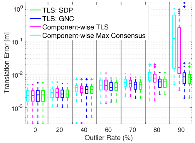
R SDP Relaxations: Quaternion vs. Rotation Matrix
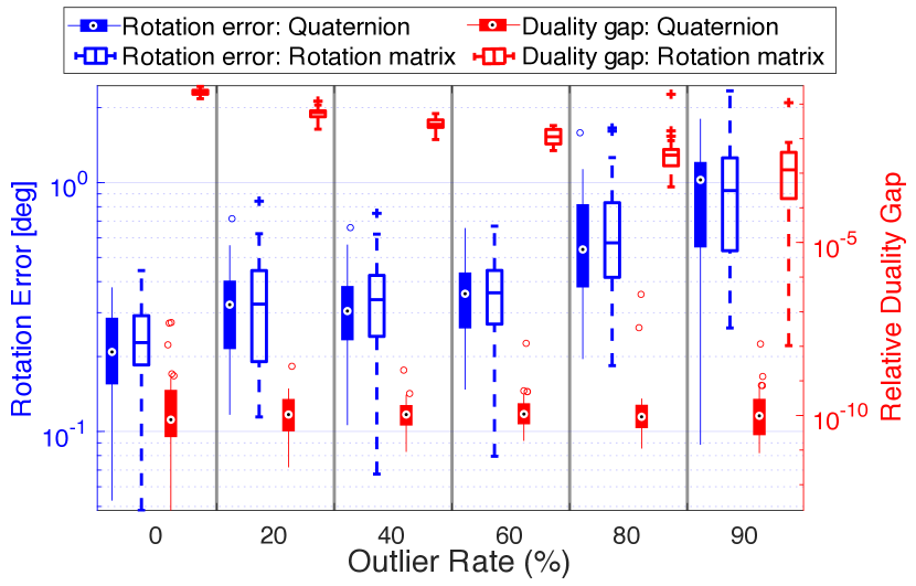 (a) Results on the Bunny dataset.
|
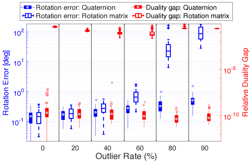 (b) Results on random simulated unit vectors.
|
In Section XI, we compare the rotation estimation error between the quaternion-based SDP relaxation (eq. (29), [39]) and the rotation-matrix-based SDP relaxation ([38]) on the Bunny dataset. In this section, we also report the relative duality gap for the two relaxations on the Bunny dataset. Fig. 13(a) shows the relative duality gap (boxes in red, scale on the right-hand y-axis) and the rotation error (boxes in blue, scale on the left-hand y-axis). The figure shows that the the quaternion-based relaxation is always tighter than the rotation-matrix-based relaxation, although both relaxations achieve similar performance in terms of rotation estimation errors.
To further stress-test the two techniques, we compare their performance in a more randomized test setting [39]: at each Monte Carlo run, we first randomly sample unit vectors from the 3D unit sphere, then apply a random rotation and isotropic Gaussian noise (standard deviation ) to the unit vectors. Fig. 13(b) shows the results under this setting. We can see that the quaternion-based relaxation remains tight, while the rotation-matrix-based relaxation has a much larger relative duality gap. In addition, a tighter relaxation translates to more accurate rotation estimation: the quaternion-based relaxation dominates the rotation-matrix relaxation and obtains much more accurate rotation estimates, especially at outlier rates.
S Stanford Dataset: Extra Results
In all the following experiments, for scale, rotation and translation estimation.
S1 Benchmark on Synthetic Datasets
As stated in Section XI-B in the main document, we have benchmarked TEASER against four state-of-the-art methods in point cloud registration (FGR [55], GORE [19], RANSAC1K, RANSAC) at increasing level of outliers, using four datasets from the Stanford 3D Scanning Repository [97]: Bunny, Armadillo, Dragon and Buddha. Results for the Bunny are showed in the main document and here we show the results for the other three datasets in Fig. 14. The figure confirms that TEASER dominates the other techniques is insensitive to extreme outlier rates.
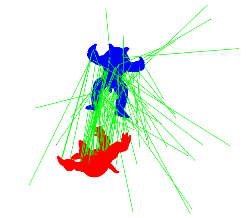
|
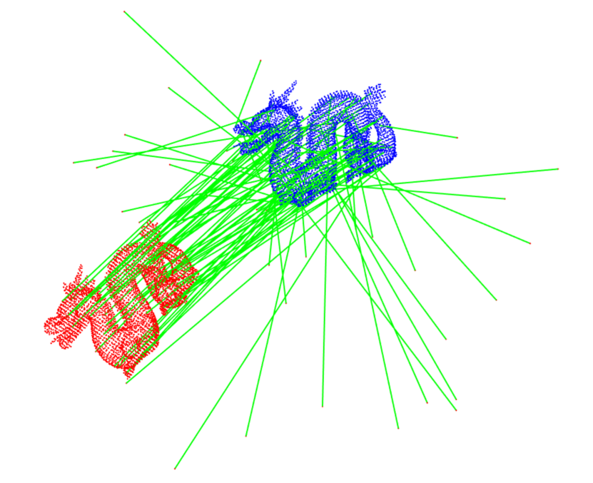
|
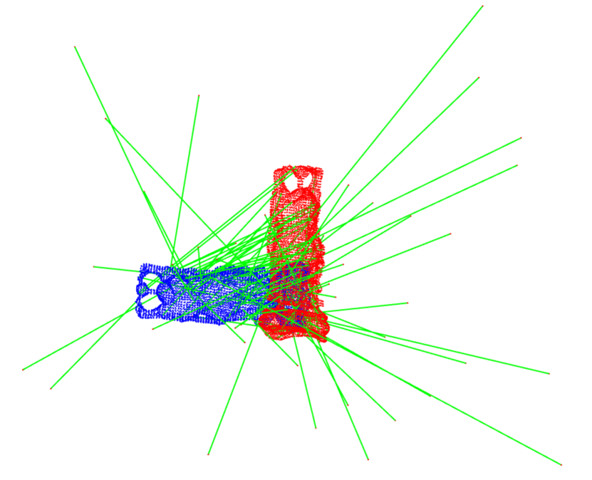
|
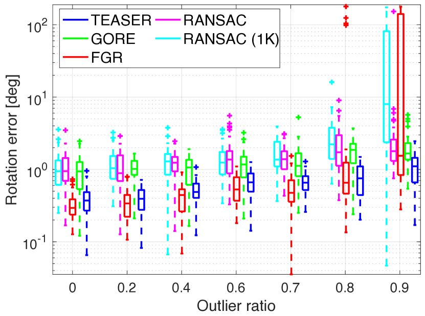
|
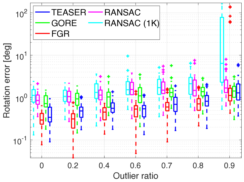
|
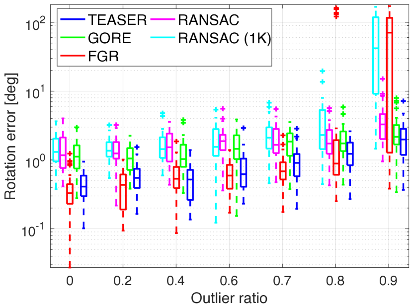
|
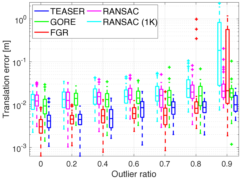 (a) Armadillo
|
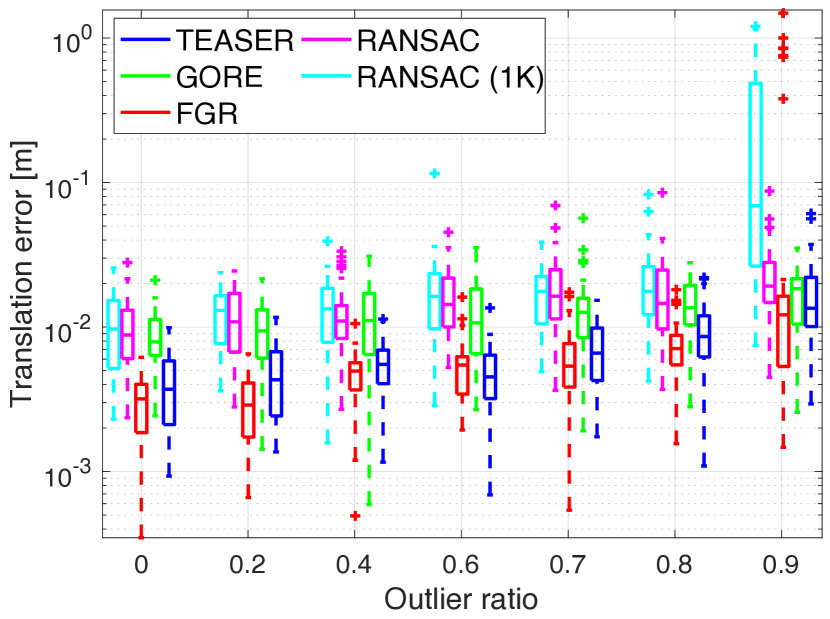 (b) Dragon
|
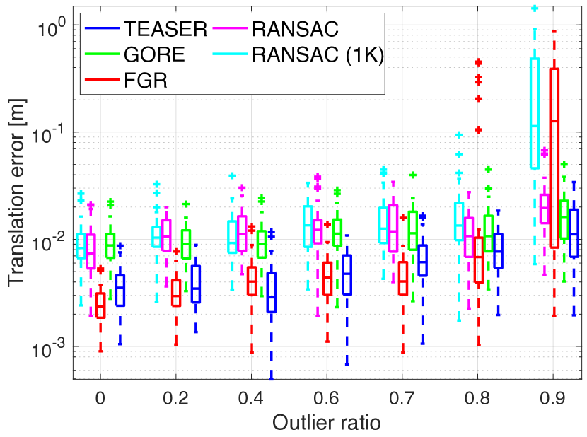 (c) Buddha
|
S2 TEASER on High Noise
In the main document, the standard deviation of the isotropic Gaussian noise is set to be , with the point cloud scaled inside a unit cube . In this section, we give a visual illustration of how corrupted the point cloud is after adding noise of such magnitude. In addition, we increase the noise standard deviation to be , visualize the corresponding corrupted point cloud, and show that TEASER can still recover the ground-truth transformation with reasonable accuracy. Fig. 17 illustrates a clean (noise-free) Bunny model (Fig. 17(a)) scaled inside the unit cube and its variants by adding different levels of isotropic Gaussian noise and outliers. From Fig. 17(b)(c), we can see (noise used in the main document) is a reasonable noise standard deviation for real-world applications, while destroys the geometric structure of the Bunny and it is beyond the noise typically encountered in robotics and computer vision applications. Fig. 17(d) shows the Bunny with high noise () and 50% outliers. Under this setup, we run TEASER to register the two point clouds and recover the relative transformation. TEASER can still return rotation and translation estimates that are close to the ground-truth transformation. However, due to the severe noise corruption, even a successful registration fails to yield a visually convincing registration result to human perception. For example, Fig. 15 shows a representative TEASER registration result with noise corruption and outlier rate, where accurate transformation estimates are obtained (rotation error is and translation error is m), but the Bunny in the cluttered scene is hardly visible, even when super-imposed to the clean model.
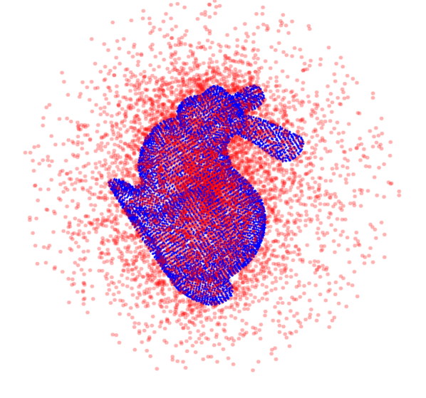
|
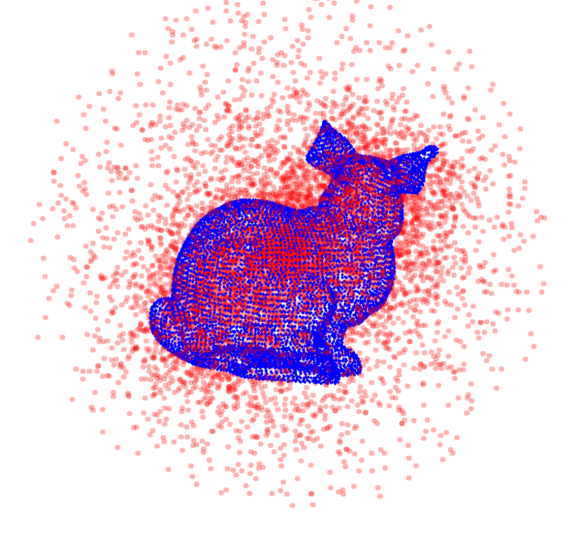
|
S3 TEASER++ on Problems with Increasing Number of Correspondences
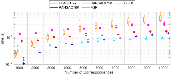
(a) Runtimes vs. number of correspondences
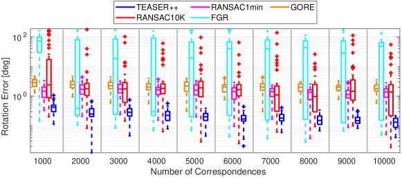
(b) Rotation errors vs. number of correspondences
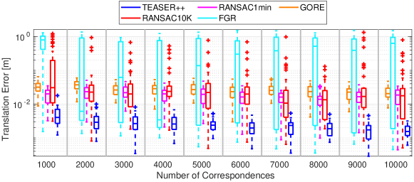
(c) Translation errors vs. number of correspondences
Here we provide more results for TEASER++ on problems with higher number of correspondences. We follow the same experimental setup as detailed in Section XI-B, with the exception that we fixed our outlier rate at 95%, and test the algorithms with increasing numbers of correspondences. Fig. 16 shows the results of the experiments.
Overall, in terms of rotation errors and translation errors, TEASER++ dominates other methods by a large margin. In terms of speed, TEASER++ outperforms other robust estimation algorithms such as GORE. While TEASER++’s runtime scales with the number of correspondences, it still outperforms methods such as GORE on all cases. At 10000 correspondences, TEASER++ only takes around 2 seconds to solve the registration problem. This demonstrates that TEASER++ can be used to solve registration problems with high number of correspondences within reasonable amount of time.
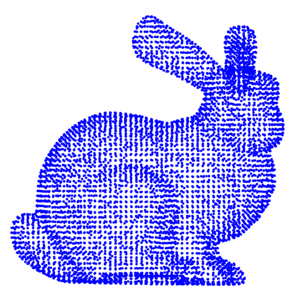 (a) Bunny model
|
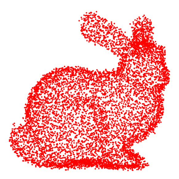 (b) Bunny scene,
|
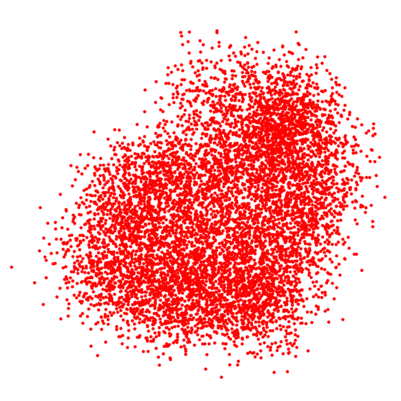 (c) Bunny scene,
|
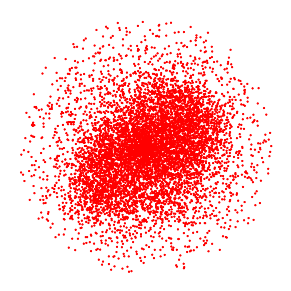 (d) Bunny scene, ,
50% outliers
(d) Bunny scene, ,
50% outliers
|
T Object Pose Estimation: Extra Results
Fig. 18 shows the registration results for the 8 selected scenes from the University of Washington RGB-D datasets [36]. The inlier correspondence ratios for cereal box are all below 10% and typically below 5%. TEASER is able to compute a highly-accurate estimate of the relative pose using a handful of inliers. Due to the distinctive shape of cap, FPFH produces a higher number of inliers and TEASER is able to register the object-scene pair without problems.
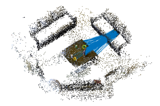
|
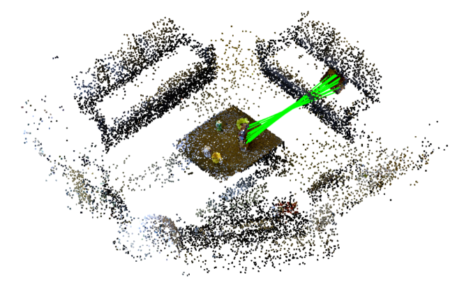
|
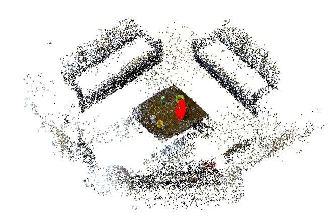
|
| scene-2, # of FPFH correspondences: 550, Inlier ratio: 4.55%, Rotation error: 0.120, Translation error: 0.052. | ||
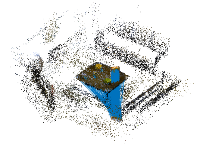
|
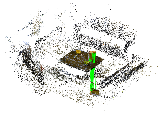
|
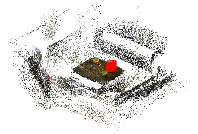
|
| scene-4, # of FPFH correspondences: 636, Inlier ratio: 4.56%, Rotation error: 0.042, Translation error: 0.051. | ||
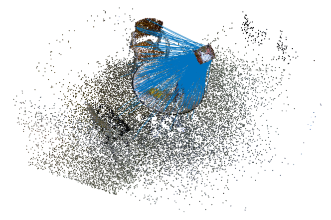
|
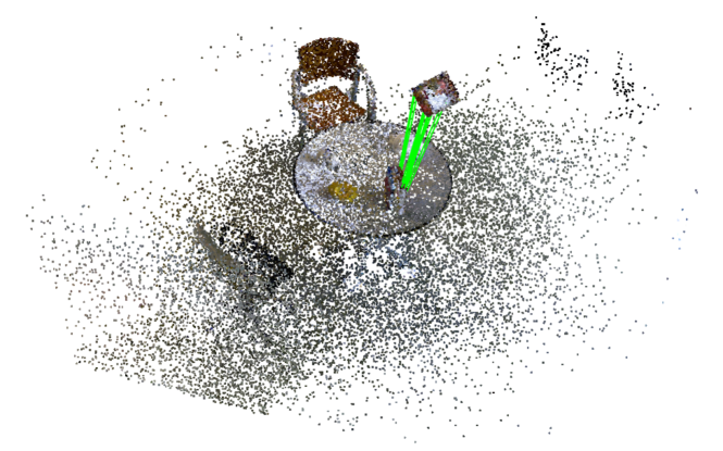
|
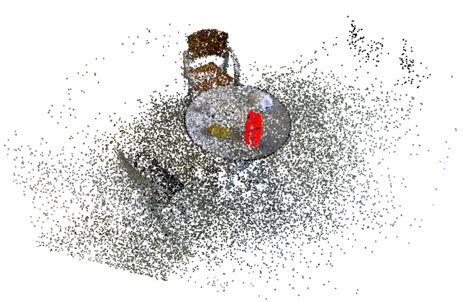
|
| scene-5, # of FPFH correspondences: 685, Inlier ratio: 2.63%, Rotation error: 0.146, Translation error: 0.176. | ||
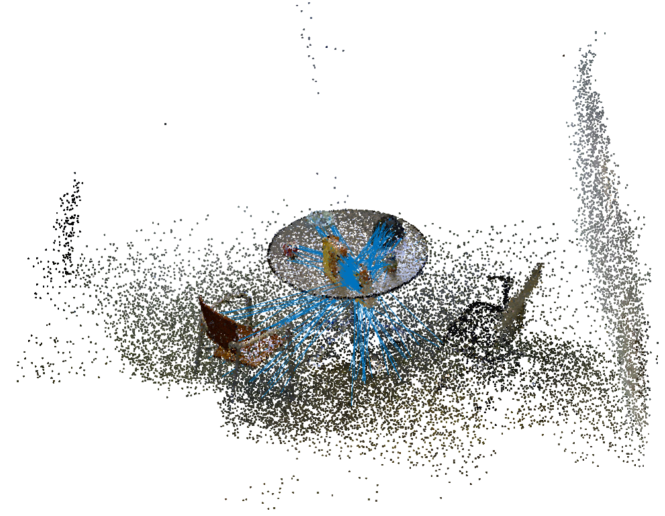
|
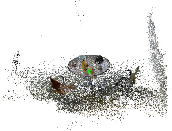
|
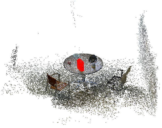
|
| scene-7, # of FPFH correspondences: 416, Inlier ratio: 3.13%, Rotation error: 0.058, Translation error: 0.097. | ||
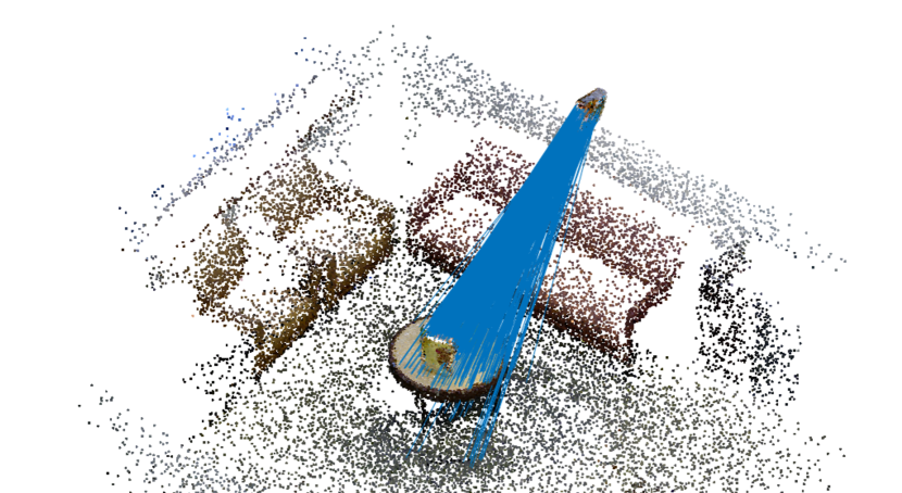
|
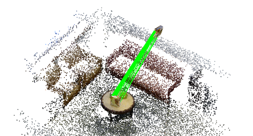
|
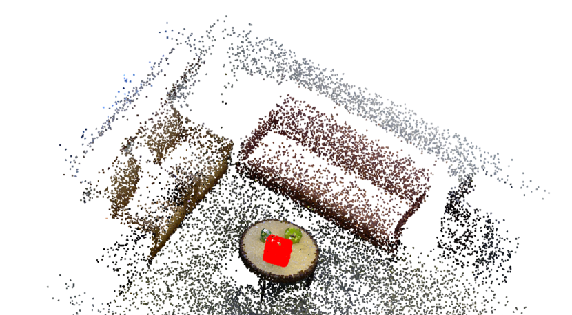
|
| scene-9, # of FPFH correspondences: 651, Inlier ratio: 8.29%, Rotation error: 0.036, Translation error: 0.011. | ||
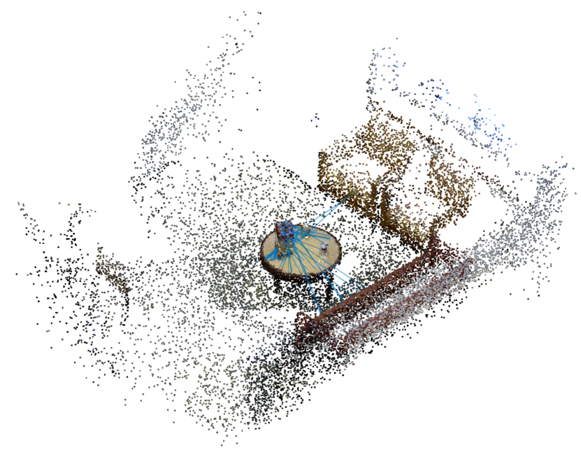
|
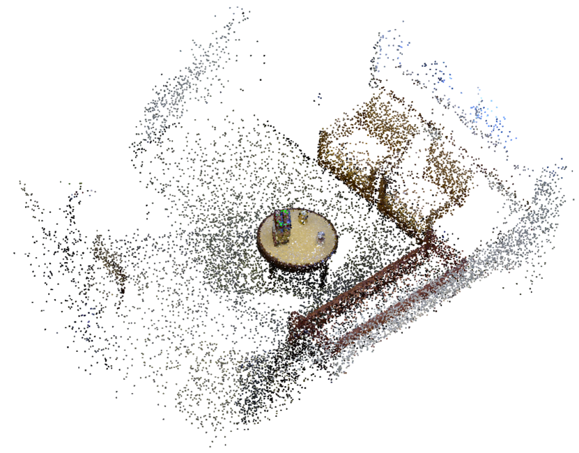
|
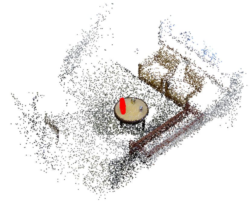
|
| scene-11, # of FPFH correspondences: 445, Inlier ratio: 6.97%, Rotation error: 0.028, Translation error: 0.016. | ||
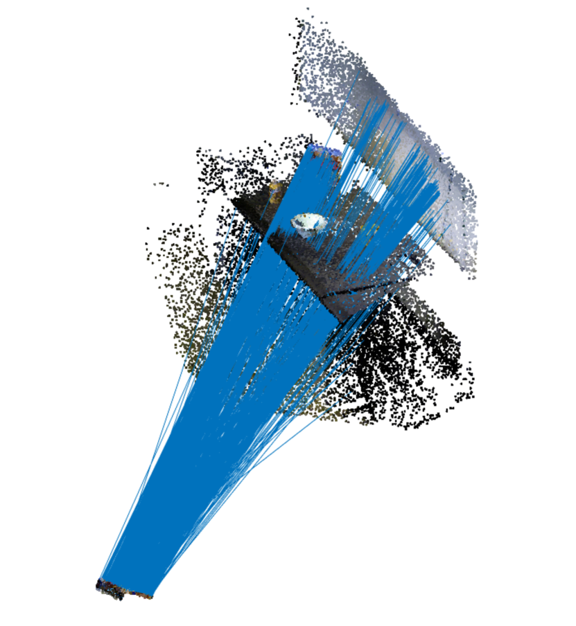
|
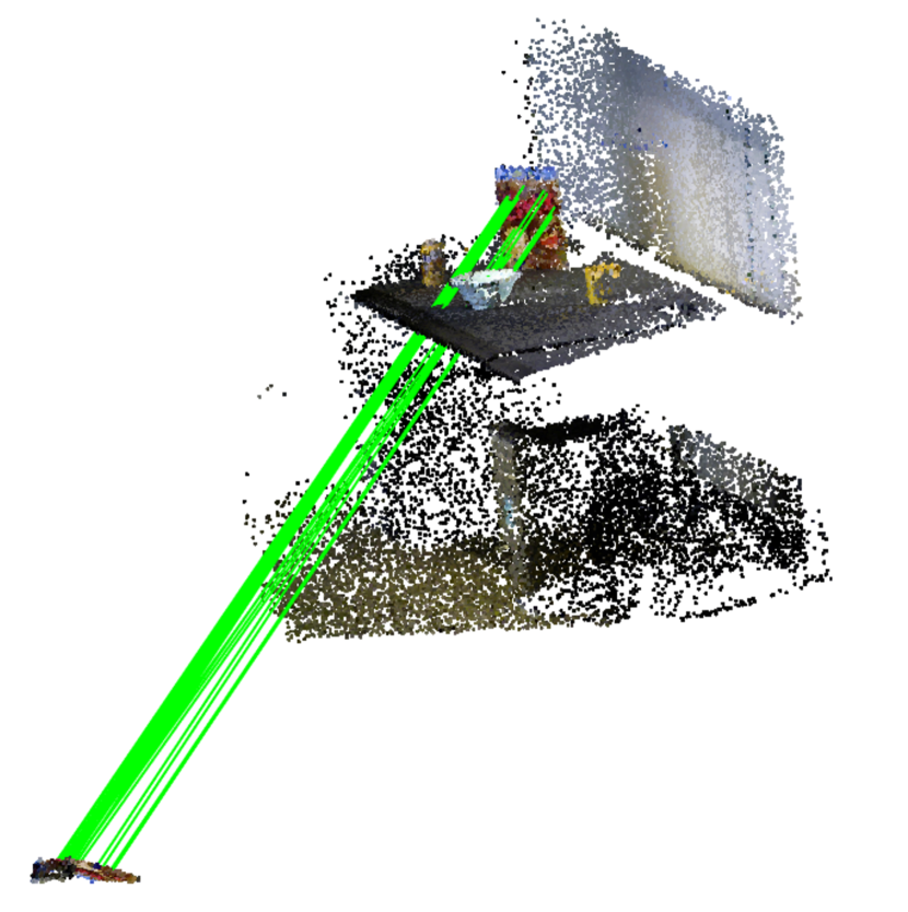
|
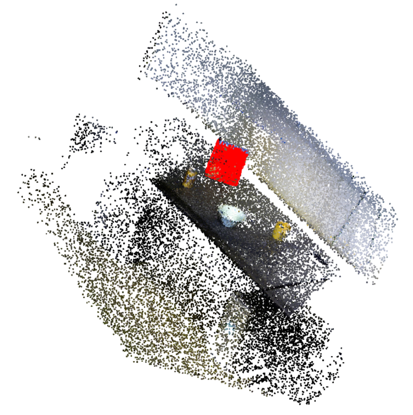
|
| scene-13, # of FPFH correspondences: 612, Inlier ratio: 5.23%, Rotation error: 0.036, Translation error: 0.064. | ||
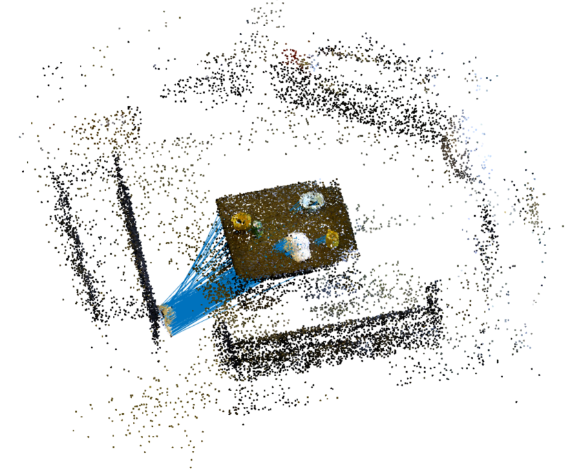
|
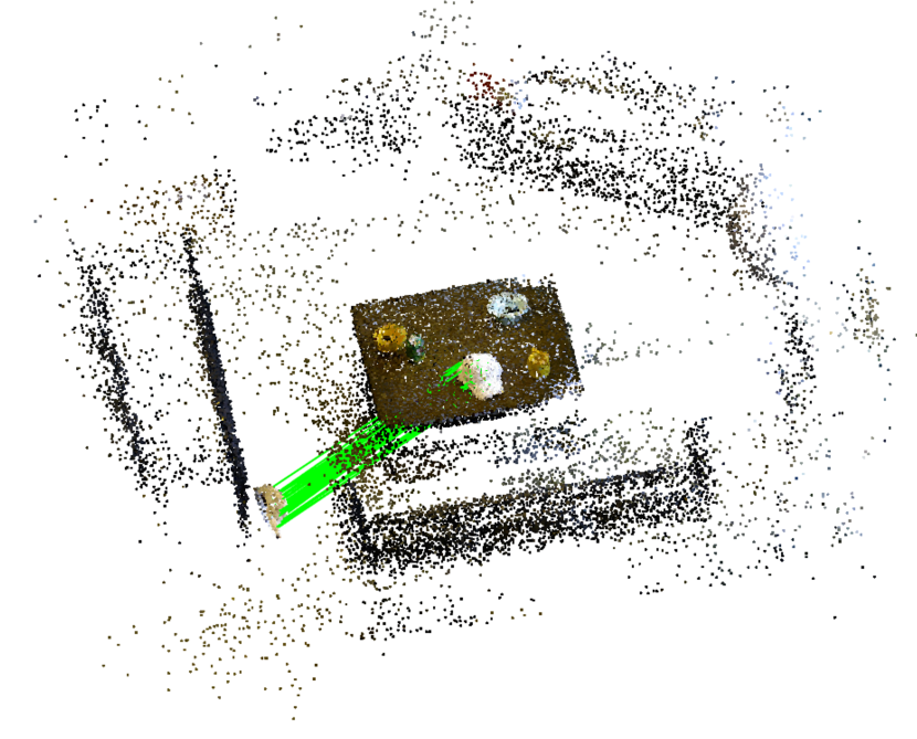
|
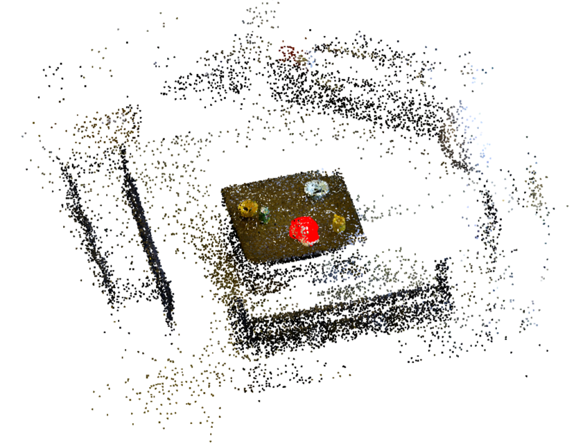
|
| scene-1, # of FPFH correspondences: 207, Inlier ratio: 16.91%, Rotation error: 0.066, Translation error: 0.090. | ||
U Proof of Proposition 33: Projection onto
Proof.
We first analyze the constraints defined by the affine subspace (98). For any matrix , can be written as , with and satisfies , we write this in matrix form:
| (165) |
where the expressions for and are given by the following:
| (166) |
Denote , we write the -th () block-row equality of (165):
| (167) | |||
| (170) | |||
| (171) |
and from eq. (171), we can get the a sum of all to be:
| (172) | |||||
and the sum of all to be:
| (173) |
Now we write the -th block row equality of (165):
| (174) | |||
| (177) | |||
| (178) | |||
| (179) |
and compare eq. (179) with eq. (172):
| (180) | |||
| (181) | |||
| (182) | |||
| (183) |
which states that for inliers , the sum must hold121212This condition is always true because this is the first-order stationary condition for the TLS optimization considering only the least squares part applied on inliers.. We then compare eq. (179) with eq. (173):
| (184) | |||
| (185) | |||
| (186) |
which holds true without any condition. Therefore, we conclude that the equality constraint of the -th block row adds no extra constraints on the matrix . This leads to the following Theorem.
Theorem 34 (Equivalent Projection to ).
The projection of a matrix onto is equivalent to:
| (187) |
where is defined by:
| (188) |
Next we prove that the projection steps in Proposition 33 define the correct projection . To this end, we use to denote the projection of a matrix onto the set . By the definition of projection, is the minimizer of the following optimization:
| (189) |
Denoting the objective function of eq. (189) as , we separate the Frobenius norm of into a sum of block-wise Frobenius norms:
| (190) | |||
| (191) |
where is the following set of ordered indices that enumerate the lower-triangular blocks of any matrix :
| (192) |
and equals to the flipped copy of (eq. (110)). Using the separated Frobenius norm (191), we can get the projection block by block in the following steps.
-
1.
Diagonal block matrix part. From the expression of and the constraint that , we can get the diagonal block matrix part of to be:
(193) which first computes the mean of all diagonal block matrix parts, , and then subtracts the mean from each individual diagonal block matrix part .
-
2.
Diagonal block scalar part. From the expression of and the constraint from eq. (171) (which fixes the scalar parts to be known constants), we can get the diagonal block scalar part of to be:
(194) which first computes the diagonal scalar parts for and then assigns the negative sum of all diagonal scalar parts to the scalar part of the top-left diagonal block ().
-
3.
Off-diagonal block matrix part. From the expression of and the constraint that is skew-symmetric, we can obtain the off-diagonal block matrix part of to be:
(195) which simply projects to its nearest skew-symmetric matrix. Note that it suffices to only project the upper-triangular off-diagonal blocks because both and are symmetric matrices.
-
4.
Off-diagonal block scalar part. The off-diagonal blocks are skew-symmetric matrices and the scalar parts must be zeros. Therefore, the off-diagonal block scalar parts of are:
(196) -
5.
Off-diagonal block vector part. The projection of the vector parts of each block is non-trivial due to the coupling between the diagonal block vector parts and the off-diagonal block vector parts . We first write the diagonal block vector parts as functions of the off-diagonal block vector parts by recalling eq. (171) and (172):
(197) which shows that we can write in a unified notation:
(198) Inserting eq. (198) into the expression of in eq. (191), and using the fact that , we obtain the following unconstrained optimization problem:
(199) To solve problem (199), we first derive the partial derivatives w.r.t. each variable . For notation simplicity, we write , where represent the block-row and block-column indices. In addition, we use to denote the pointer that returns the index of in the set . Using this notation, the partial derivative of w.r.t. is:
(200) (201) (202) Notice that not all of the and in eq. (202) belong to the upper-triangular part of , therefore, we use the fact that for any to convert all lower-triangular vectors to upper-triangular. In addition, we set the partial derivative to zero to obtain sufficient and necessary conditions to solve the convex unconstrained optimization (199):
(203) (204) (205) (206) where the linear map is as defined in eq. (111), and is defined as in eq. (203), and is the following vector:
(207) where denotes the -th entry of vector . Because the partial derivative w.r.t. each variable , must be zero at the global minimizer, , of problem (199), we have linear equations of the form eq. (206), which allows us to write the following matrix form:
(208) and we can compute by:
(209) Surprisingly, due to the structure of , its inverse can be computed in closed form.
Theorem 35 (Closed-form Matrix Inverse).
The inverse of matrix (207), denoted , can be computed in closed form, with each column of being:
(210) where and are the following constants:
(211) Proof.
To show is the inverse of , we need to show . To do so, we first show that , which means the diagonal entries of are all equal to 1. Note that from the definition of in (207) and in (210), one can see that there are non-zero entries in and and when , and when , therefore, we have:
(212) We then show that for any . The non-zero indices of , and their corresponding entries are:
(225) where we have used and . Now depending on the 12 different relations between and , and can have different ways of sharing common indices whose corresponding entries in both and are non-zero. We next show that in all these 12 different cases, holds true.
-
(a)
: and share 4 non-zero entries with the same indices:
(231) Using the above table, we easily see that .
-
(b)
: and share the following common indices whose corresponding entries are non-zero:
(238) Using the table above, we can calculate :
(239) which ends up being due to (cf. eq. (211)).
-
(c)
: and share 4 common indices with non-zero entries:
(245) from which we can compute that .
-
(d)
: and share the following common indices with non-zero entries:
(252) from which we can compute :
(253) -
(e)
: and share the following common indices with non-zero entries:
(260) from which we compute :
(261) -
(f)
: and share 4 common indices with non-zero entries:
(267) from which we easily see that .
-
(g)
: same as by symmetry (switch and ).
-
(h)
: same as by symmetry.
-
(i)
: same as by symmetry.
-
(j)
: same as by symmetry.
-
(k)
: same as by symmetry.
-
(l)
: same as by symmetry.
As we show above, in all cases, , when . Therefore, we prove that and is the closed-form inverse of .
-
(a)
-
6.
Diagonal block vector part. After obtaining off-diagonal block vector parts, we can insert them back into eq. (198) to obtain the diagonal block vector parts:
(268) (269)
V Initial Guess for Algorithm 3
We describe the initial guess as:
| (270) |
where is the following:
| Off-diagonal blocks: | (271) | ||||
| Diagonal block scalar part: | (272) | ||||
| Diagonal block vector part: | (273) | ||||
| Diagonal block matrix part: | (274) |
One can verify that satisfies all the constraints defined by set (188).
W Tighter Bounds for Theorem 17
In this section, we improve over the bounds presented in Theorem 17 and derive tighter but more complex bounds for scale, rotation, and translation estimation.
Theorem 36 (Estimation Contract with Noisy Inliers and Adversarial Outliers).
Assume (i) the set of correspondences contains at least 3 distinct and non-collinear inliers, where for any inlier , , and denotes the ground truth transformation. Assume (ii) the inliers belong to the maximum consensus set in each subproblem131313In other words: the inliers belong to the largest set such that for any , , , and for any transformation . Note that for translation the assumption is applied component-wise. , and (iii) the second largest consensus set is “sufficiently smaller” than the maximum consensus set (as formalized in Lemma 23). If (iv) the rotation subproblem produces a valid certificate (as per Theorems 13-14), then the output of TEASER satisfies:
| (275) | |||
| (276) | |||
| (277) |
where is the set of ground-truth inliers with size , i.e., ground-truth TRIMs in the scale bound, ground-truth TIMs in the rotation bound, and ground-truth correspondences in the translation bound; denotes the -th entry of the translation vector; , and are defined as follows:
| (278) |
is the angular (geodesic) distance between and ; is the matrix that assembles all normalized TIMs in the set , and , denotes the smallest and second smallest singular values of matrix . Note that since there are at least 3 non-collinear ground-truth inliers, and , meaning the rotation bound is well defined. Since the bounds rely on the knowledge of the inliers , to compute the worst-case bounds, one has to enumerate over all possible subsets of inliers to compute the largest bounds for scale, rotation and translation.
Proof.
We will prove the bounds for scale, rotation, and translation separately.
Scale Error Bound. Let us denote with the consensus set associated with the optimal solution of the TLS scale estimation problem, with . To establish a connection with the ground-truth scale , we partition into two sets: that contains all the indices of the true inliers, and that contains all the indices of the false inliers, which are not generated from the true inlier model (TRIM) where classified as inliers by TLS and ended up in . Let and , and we have . For scale measurements that are in and , we have the following relations:
| (279) |
where ’s and ’s are residuals that can be computed from and , and ’s are unknown noise terms. Note that we have . From the first equation in eq. (279), we have:
| (280) | |||
| (281) |
where we have defined a new quantity , that can be computed for every TRIM in the consensus set . Eq. (280) states that the scale error is bounded by the minimum in the set of true inliers. Therefore, if we know what the set of true inliers is, then we can simply take the minimum of the set . However, if we do not know the true inlier set, assuming , we get the worst-case bound:
| (282) |
where is the third-largest in the set .
Rotation Error Bound. Similar to the previous case, we use to denote the consensus set of TIM at the optimal TLS estimate. We also use to denote the set of true inliers and use to denote the set false inliers, i.e., outliers that TLS selected as inliers. We have the following equations for the true inliers and false inliers:
| (283) |
where are the residuals that can be computed and is the unknown noise term. From the first equation of eq. (283), we have:
| (284) | |||
| (285) |
where and we have defined a new quantity that can be computed from the TLS solution. Since eq. (285) holds for every TIM in , we can aggregate all inequalities:
| (286) |
where assembles all normalized TIMs in the set . Now we want to get a lower bound on so that we can upper-bound the rotation error.
Towards this goal, we first analyze the singular values of . Let the three singular values of be , then we know that are equal to the eigenvalues of the matrix . Expanding , we get:
| (287) |
where we have denoted , which is the composition of two rotation matrices. Let the axis-angle representation of be , then the axis-angle representation for is simply . According to the Rodrigues’ rotation formula, we can write and as:
| (288) |
Inserting eq. (288) back into eq. (287), we have:
| (289) |
from which we can see that the three eigenvectors of are and and , where we pick and to be 2 unit orthogonal vectors in the plane that is orthogonal to :
| (290) |
Therefore, we have and . Let the SVD of be , we lower-bound :
| (297) | |||
| (298) | |||
| (299) | |||
| (300) |
where we have used , with being the three singular values of in ascending order. The last inequality in eq. (300) follows from:
| (307) |
Now we combine eq. (300) and (286) to bound :
| (308) | |||
| (309) |
where we note that (i) the existence of at least 3 non-collinear inliers guarantees that , which means and the upper bound is well-defined; (ii) since is the axis-angle representation for , is the angular (geodesic) distance between and ; (iii) the rotation bound is dependent on the scale bound (281).
Again, when the true inlier set is known, one can directly compute the rotation bound using eq. (309); when the true inlier set is unknown, one has to enumerate over all possible subsets of 3 TIMs (formed by a triplet of correspondences) in to compute the worst-case bound.
Translation Error Bound. Let and be the ground-truth and estimated translation. Let be the set of measurements that pass the -th component-wise adaptive voting, i.e., . Again, we let and be the set of true and false inliers within . From condition (ii), we have that , which says that the true inliers pass all three component-wise adaptive voting. However, could potentially be different. Then we write the following relations:
| (310) |
where is the unknown noise that satisfies and and are the residuals that can be computed from the TLS estimate and satisfy and . From the first equation in (310), we have that:
| (311) | |||
| (312) |
where we have defined a new quantity that can be computed from the solution. Now we want to upper-bound , using a similar SVD-based approach as in eq. (300) (but this time we upper-bound):
| (313) | |||
| (314) |
Inserting the inequality (314) back into eq. (312), we get the following translation bound for each
| (315) |
there the final translation bound is:
| (316) |
We note that the translation bound depends on both the scale bound (281) and the rotation bound (309). When the true inlier set is known, one can directly compute the bound using eq. (315); when the true inlier set is unknown, one has to enumerate over all possible subsets of 3 inliers in to compute the worst-case translation bound.