JWvG:1749

Dynamics of a stochastic excitable system with slowly adapting feedback

Abstract

We study an excitable active rotator with slowly adapting nonlinear feedback and noise. Depending on the adaptation and the noise level, this system may display noise-induced spiking, noise-perturbed oscillations, or stochastic busting. We show how the system exhibits transitions between these dynamical regimes, as well as how one can enhance or suppress the coherence resonance, or effectively control the features of the stochastic bursting. The setup can be considered as a paradigmatic model for a neuron with a slow recovery variable or, more generally, as an excitable system under the influence of a nonlinear control mechanism. We employ a multiple timescale approach that combines the classical adiabatic elimination with averaging of rapid oscillations and stochastic averaging of noise-induced fluctuations by a corresponding stationary Fokker-Planck equation. This allows us to perform a numerical bifurcation analysis of a reduced slow system and to determine the parameter regions associated with different types of dynamics. In particular, we demonstrate the existence of a region of bistability, where the noise-induced switching between a stationary and an oscillatory regime gives rise to stochastic bursting.

Recent years have witnessed a rapid expansion of stochastic models for a wide variety of important physical and biological phenomena, from sub-cellular processes and tissue dynamics, over large-scale population dynamics and genetic switching to optical devices, Josephson junctions, fluid mechanics and climatology. These studies have demonstrated that the effects of noise manifest themselves on a broad range of scales, but nevertheless display certain universal features. In particular, the effects of noise may generically be cast into two groups. On the one hand, the noise may enhance or suppress the features of deterministic dynamics, while on the other hand, it may give rise to novel forms of behavior, associated with the crossing of thresholds and separatrices, or with stabilization of deterministically unstable states. The constructive role of noise has been evinced in diverse applications, from neural networks and chemical reactions to lasers and electronic circuits. Classical examples of stochastic facilitation in neuronal systems concern resonant phenomena, such as coherence resonance, where an intermediate level of noise may trigger coherent oscillations in excitable systems, as well as spontaneous switching between the coexisting metastable states. In the present study, we show how the interaction of noise and multiscale dynamics, induced by slowly adapting feedback, may affect an excitable system. It gives rise to a new mode of behavior based on switching dynamics, namely the stochastic bursting, and allows for an efficient control of the properties of coherence resonance.

I Introduction

Multiscale dynamics is ubiquitous in real-world systems. In neuron models, for instance, the evolution of recovery or gating variables is usually much slower than the changes of the membrane potential (Izhikevich, 2007; Gerstner et al., 2014). At the level of neural networks, certain mechanisms of synaptic adaptation, such as the spike timing-dependent plasticity (Abbott and Dayan, 2005; Clopath et al., 2010; Popovych et al., 2013), are slower than the spiking dynamics of individual neurons. When modeling the dynamics of semiconductor lasers (Lang and Kobayashi, 1980; Lüdge, 2011; Soriano et al., 2013), one similarly encounters at least two different timescales, one related to the carriers’ and the other to the photons’ lifetime, whereby their ratio can span several orders of magnitude. Investigating the dynamics of such multiscale systems has lead to the development of a number of useful asymptotic and geometric methods, see Refs. (Krupa et al., 1997; Lichtner et al., 2011; Desroches et al., 2012; Kuehn, 2015; Jardon-Kojakhmetov and Kuehn, 2019) to name just a few.

Another ingredient inevitable in modeling real-world systems is noise, which may describe the intrinsic randomness of the system, the fluctuations in the embedding environment, or may derive from coarse-graining over the degrees of freedom associated with small spatial or temporal scales (Haken, 1985; Lindner et al., 2004). For instance, neuronal dynamics is typically influenced by intrinsic sources of noise, such as the random opening of ion channels, and by external sources, like the synaptic noise (Destexhe and Rudolph-Lilith, 2012). In chemical reactions, noise comprises finite-size effects, while the stochasticity in laser dynamics reflects primarily quantum fluctuations. In general, the impact of noise can manifest itself by modification of the deterministic features of the system, or by the emergence of qualitatively novel types of behavior, induced by the crossing of thresholds or separatrices (Forgoston and Moore, 2018).

In the present paper, we study the effects of slowly adapting feedback and noise on an excitable system. Excitability is a general nonlinear phenomenon based on a threshold-like response of a system to a perturbation (Murray, 1989; Winfree, 2001; Lindner et al., 2004; Izhikevich, 2007). An excitable system features a stable "rest" state intermitted by excitation events (firing), elicited by perturbations. In the absence of a perturbation, such a system remains in the rest state and a small perturbation induces a small-amplitude linear response. If the perturbation is sufficiently strong, an excitable system reacts by a large-amplitude nonlinear response, such as a spike of a neuron. When an excitable system receives additional feedback or a stochastic input, or is coupled to other such systems, new effects may appear due to the self- or noise-induced excitations, as well as excitations from the neighboring systems. Such mechanisms can give rise to different forms of oscillations, patterns, propagating waves, and other phenomena (Lindner et al., 2004; Pikovsky and Kurths, 1997; Oriol et al., 2011; Ermentrout and Kleinfeld, 2001; Lücken et al., 2017; Franović et al., 2018; Bačić et al., 2018; Franović et al., 2015a, b; Yanchuk et al., 2019).

Our focus is on a stochastic excitable system subjected to a slow control via a low-pass filtered feedback

$$\dot{v} =f(v,\mu)+\sqrt{D}\xi(t),$$ (1)

$$\dot{\mu} =\varepsilon(-\mu+\eta g(v)),$$ (2)

where $\varepsilon\gtrsim 0$ is a small parameter that determines the timescale separation between the fast variable $v(t)$ and the slow feedback variable $\mu(t)$. The fast dynamics $\dot{v}=f(v,0)$ is excitable and is influenced by the Gaussian white noise $\xi(t)$ of variance $D$. Moreover, the slow feedback variable $\mu$ controls its excitability properties. The parameter $\eta$ is the control gain, such that for $\eta=0$ one recovers a classical noise-driven excitable system (Lindner et al., 2004). An important example of a system conforming to (1)–(2) for $\eta\neq 0$ is the Izhikevich neuron model (Izhikevich, 2004), where the stochastic input to the fast variable would describe the action of synaptic noise.

Here we analyze a simple paradigmatic example from the class of systems (1)–(2), where the excitable local dynamics is represented by an active rotator

$$\dot{\varphi}=I_{0}-\sin\varphi\quad\textrm{with}\quad\varphi\in S^{1}.$$

The latter undergoes a saddle-node infinite period (SNIPER) bifurcation at $|I_{0}|=1$, turning from excitable ($|I_{0}|\lesssim 1$) to oscillatory regime $|I_{0}|>1$, see (Strogatz, 1994). The adaptation is represented by a positive periodic function $g(\varphi)=1-\sin\varphi$, such that the complete model reads

$$\dot{\varphi} =I_{0}-\sin\varphi+\mu+\sqrt{D}\xi(t),$$ (3)

$$\dot{\mu} =\varepsilon\left(-\mu+\eta\left(1-\sin\varphi\right)\right).$$ (4)

In the presence of feedback, the noiseless dynamics of the active rotator depends not only on $I_{0}$, but is affected by the term $I_{0}+\mu$ involving the control variable $\mu(t)$, which can induce switching between the excitable equilibrium ($|I_{0}+\mu|<1$) and the oscillatory regime ($|I_{0}+\mu|>1$). This adaptation rule provides a positive feedback for the spikes and oscillations, since $\mu$ increases when $\varphi(t)$ is oscillating and drives the system towards the oscillatory regime, while in the vicinity of the equilibrium ($\sin\varphi\approx 1$) the control signal effectively vanishes.

We examine how the behavior of (3)-(4) is influenced by the noise level $D$ and the control gain $\eta$, determining the phase diagram of dynamical regimes in terms of these two parameters. The first part of our results in Sec. II concerns the noise-free system $D=0$, where we employ a combination of two multiscale methods, namely adiabatic elimination in the regime where the fast subsystem has a stable equilibrium and the averaging approach when the fast subsystem is oscillatory. As a result, we obtain a reduced slow system that is capable of describing both the slowly changing fast oscillations and the slowly drifting equilibrium, as well as the transitions between these regimes. The bifurcation analysis of this slow system reveals the emergence of a bistability between the fast oscillations and the equilibrium for sufficiently large $\eta$.

The second part of our results, presented in Sec. III, addresses the multiscale analysis of the dynamics in the presence of noise ($D\neq 0$). Instead of deterministic averaging, we apply the method of stochastic averaging (Shilnikov and Kolomiets, 2008; Pavliotis and Stuart, 2008; Galtier and Wainrib, 2012; Lücken et al., 2016; Bačić et al., 2018), where the distribution density for the fast variable obtained from a stationary Fokker-Plank equation is used to determine the dynamics of the slow flow. In this way, we obtain a deterministic slow dynamics for which one can perform a complete numerical bifurcation analysis with respect to $D$ and $\eta$. In section IV we investigate the effects of stochastic fluctuations on the slow dynamics, which vanish in the limit of infinite timescale separation $\varepsilon\rightarrow 0$ employed in Sec. III. The effect of a slowly adapting feedback on the coherence resonance is shown by extracting from numerical simulations the coefficient of variation of the spike time distribution in the excitable regime. In particular, we compare the results for small positive $\varepsilon$ with the case of infinite time scale separation, where we use the stationary but noise dependent $\mu$ obtained in the preceeding section. The noise-induced switching dynamics in the bistability region is demonstrated by numerical simulations showing an Eyring-Kramers type of behavior.

In terms of the different dynamical regimes, our study of stochastic dynamics reveals three characteristic $(D,\eta)$ regions featuring noise-induced spiking, noise-perturbed spiking and stochastic busting, see Figure 1. We show that by varying the control gain within the region of noise-induced spiking, one can enhance or suppress the coherence resonance, while within the bistability region, one can efficiently control the properties of stochastic bursting. The following sections provide a detailed analysis of the described phenomena.

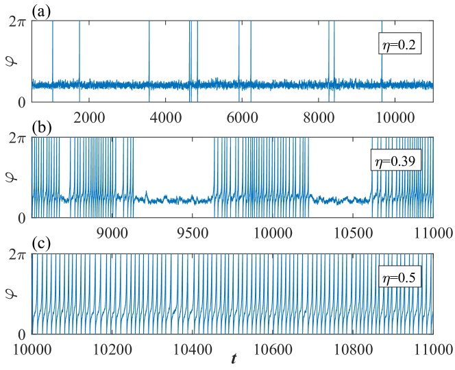
Figure 1: Different dynamical regimes in the stochastic excitable system subjected to a slow control via a low-pass filtered feedback (3)-(4) with $\varepsilon=0.005,\,D=0.008,$ and different choices of the control gain $\eta$: noise-induced spiking (a), stochastic bursting (b), and noise-perturbed spiking (c).

II Slow-fast analysis of the deterministic dynamics

In this Section, we analyze the system (3)–(4) in the absence of noise $(D=0)$

$$\dot{\varphi(t)} =I_{0}-\sin\varphi(t)+\mu(t),$$ (5)

$$\dot{\mu(t)} =\varepsilon\left(-\mu(t)+\eta\left(1-\sin\varphi(t)\right)\right),$$ (6)

considering the limit $\varepsilon\rightarrow 0$ within the framework of singular perturbation theory. The dynamics on the fast timescale is described by the so-called layer equation, obtained from (5)–(6) by setting $\varepsilon=0$

$$\dot{\varphi}(t)=I_{0}+\mu-\sin\varphi(t),$$ (7)

whereby $\mu$ acts as a parameter.

II.1 Dynamics for $\mu<1-I_{0}$: adiabatic elimination

In the case $\mu<1-I_{0}$, the layer equation (7) possesses two equilibria

$$\varphi_{+}(\mu)=\arcsin(I_{0}+\mu),\,\,\,\varphi_{-}(\mu)=\pi-\varphi_{+}(\mu),$$ (8)

where $\varphi_{+}$ is stable and $\varphi_{-}$ is unstable. Considering them as functions of the parameter $\mu$, the equilibria give rise to two branches, which merge in a fold at $\mu=1-I_{0}$, see Fig. 2. Equivalently, the set of equililbria of the fast subsystem

$$\left\{(\varphi,\mu):\,\sin\varphi=I_{0}+\mu\right\}$$ (9)

comprises the critical manifold of (5)–(6), with the stable part $\varphi_{+}(\mu)$ and the unstable part $\varphi_{-}(\mu)$..

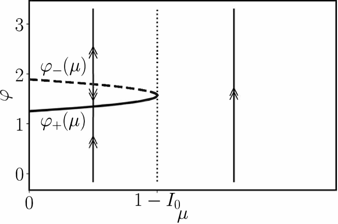
Figure 2: Critical manifold and fast dynamics of system (5)–(6). For $\mu<1-I_{0}$ the fast dynamics converges to the stable branch of the critical manifold, while for $\mu>1-I_{0}$, it is oscillatory with periodic rotation of the phase $\varphi$.

Hence, for $\mu<1-I_{0}$ the trajectories are rapidly attracted towards the stable branch of the critical manifold, along which for positive $\varepsilon$ they slowly drift. In order to describe this slow dynamics, we rescale time $T=\varepsilon t$ and obtain

$$\varepsilon\varphi^{\prime}(T) =I_{0}+\mu(T)-\sin\varphi(T),$$ (10)

$$\mu^{\prime} (T)=-\mu(T)+\eta(1-\sin\varphi(T)),$$ (11)

where the prime denotes the derivative with respect to the slow time $T$. Setting $\varepsilon=0$, we can directly eliminate the term $\sin\varphi=I_{0}+\mu$ and obtain the equation for the slow dynamics on the critical manifold

$$\mu^{\prime}(T)=-\mu(T)+\eta(1-I_{0}-\mu(T)).$$ (12)

II.2 Dynamics for $\mu>1-I_{0}$: averaging fast oscillations

For $\mu>1-I_{0}$, there is no stable equilibrium of the fast subsystem (7), see Fig. 2. Instead, one finds periodic oscillations

$$\varphi_{\mu}(t)=2\arctan\frac{1+\Omega(\mu)\tan\frac{t}{2}\Omega(\mu)}{I_{0}+\mu}$$ (13)

with the $\mu$-dependent frequency

$$\Omega(\mu)=\sqrt{(I_{0}+\mu)^{2}-1}.$$

In this case, the fast oscillations $\varphi_{\mu}(t)$ should be averaged in order to obtain the dynamics of the slow variable $\mu(T)$. A rigorous formal derivation is provided in Appendix A, finally arriving at

$$\mu^{\prime} (T)=-\mu(T)+\eta(1-I_{0}-\mu(T)+\Omega(\mu(T))).$$ (14)

Here we give a simplified explanation of the averaging procedure. First, we substitute the fast-oscillating solution $\varphi=\varphi_{\mu}(t)$ of the layer equation into the equation for the slow variable (11):

$$\mu^{\prime}(T)=-\mu(T)+\eta(1-\sin\varphi_{\mu}(t)).$$

Since the term $\sin(\cdot)$ is fast oscillating, the last equation can be averaged over the fast timescale $t,$which leads to

$$\mu^{\prime}(T)=-\mu(T)+\eta\left(1-\left\langle\sin\varphi_{\mu}(t)\right\rangle_{t}\right).$$ (15)

The average $\left\langle\sin\varphi_{\mu}(t)\right\rangle_{t}$ can be found by integrating (7) over the period

$$\langle\dot{\varphi}(t)\rangle_{t}=\Omega(\mu)=I_{0}+\mu-\langle\sin\varphi_{\mu}(t)\rangle_{t}.$$ (16)

Hence, by substituting

$$\langle\sin\varphi_{\mu}(t)\rangle_{t}=I_{0}+\mu(T)-\Omega(\mu(T))$$

into (15) we obtain the slow averaged dynamics (14).

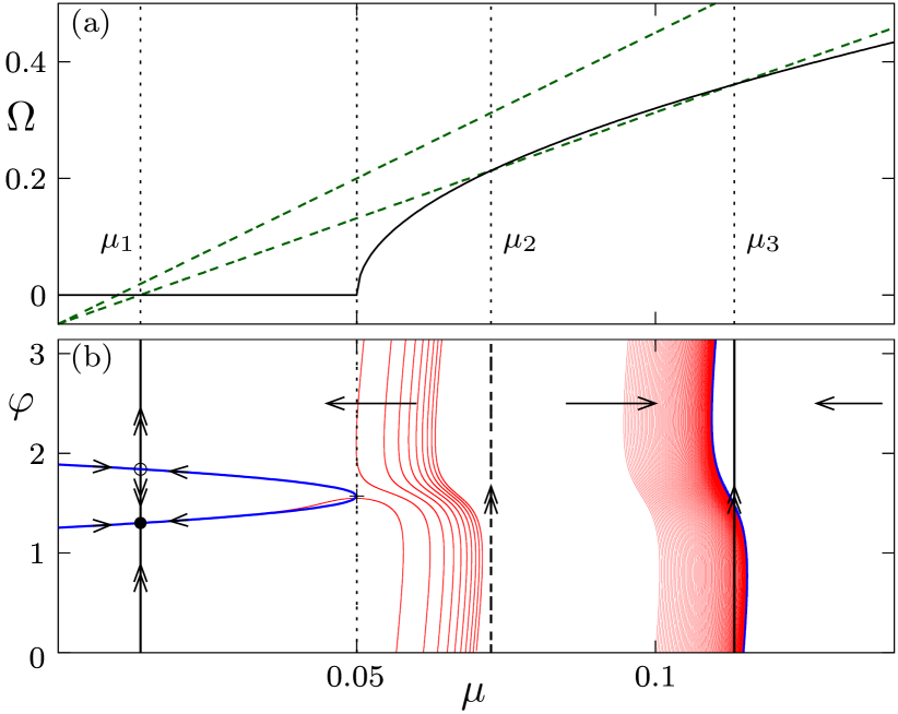
Figure 3: (a) Graphical solution of the fixed point equation (18): $\Omega(\mu)$ according to (17) (black) and the righ-hand side of (18) for different choices of $\eta$. One finds from one to three fixed points depending on $\eta$. (b) Scheme of the slow-fast dynamics of system (5),(6) with parameters $I_{0}=0.95$ and $\eta=0.38$ and the numerical sample trajectories for $\varepsilon=0.005$ (red). For $\mu<1-I_{0}$, trajectories are attracted to the stable branch of the slow manifold (blue curve) and subsequently slowly drift toward the stable fixed point $(\varphi_{+}(\mu_{1}),\mu_{1})$ (black dot). For $\mu>1-I_{0}$, the sample trajectories show fast oscillations in $\varphi$ with a slow average drift in $\mu$ in the direction indicated by the arrows.

II.3 Combined dynamics of the slow variable

Summarizing the results so far, the equation (12) describes the dynamics of the slow variable for $\mu<1-I_{0}$, while the equation (14) holds for $\mu>1-I_{0}$. These two equations can be conveniently combined into a single equation of the form (14) by extending the definition of the frequency $\Omega(\mu)$ as follows

$$\Omega(\mu)=\left\{\begin{array}[]{lr}0,&\mu<1-I_{0}\\ \sqrt{(I_{0}+\mu)^{2}-1},&\mu>1-I_{0}\end{array}\right..$$ (17)

Hence, the slow dynamics is described by the scalar ordinary differential equation on the real line (14), and, as a result, the only possible attractors are fixed points, which are given by the zeros of the right-hand side:

$$\Omega(\mu)=\frac{\eta+1}{\eta}\mu+I_{0}-1$$ (18)

Geometrically, they are points of intersection of the frequency profile $\Omega(\mu)$ with the line $\frac{\eta+1}{\eta}\mu+I_{0}-1$, see Fig. 3(a). In particular, one can check that there is always one fixed point

$$\mu_{1}=\frac{\eta(1-I_{0})}{1+\eta}<1-I_{0}$$ (19)

for which $\Omega(\mu_{1})=0$, such that it corresponds to a pair of equilibria on the critical manifold (9). Since $\mu_{1}$ is stable for the slow dynamics, the point $(\varphi_{+}(\mu_{1}),\mu_{1})$ is also a stable equilibrium for the original system (5)–(6) with small $\varepsilon$. The other two fixed points of the slow equation

$$\mu_{2,3}=\frac{\eta\left(1+\eta-I_{0}\mp\sqrt{(\eta+I_{0})^{2}-1-2\eta}\right)}{1+2\eta}$$ (20)

with $\Omega(\mu_{2,3})>0$ appear in a saddle-node bifurcation at

$$\eta_{\textrm{sn}}=1-I_{0}+\sqrt{2(1-I_{0})},$$ (21)

and correspond to a pair of periodic orbits of the layer equation (7).

In Fig. 3(b) we show schematically the results of our slow-fast analysis for $I_{0}=0.95$ and $\eta=0.38$. For the chosen parameter values there are two stable regimes: the fixed point $(\varphi_{+}(\mu_{1}),\mu_{1})$ and a fast oscillation with $\langle\mu(t)\rangle_{t}\approx\mu_{3}$.

Finally, Fig. (4) presents the bifurcation diagram of the fixed points of the slow dynamics with respect to the control gain $\eta$. One observes that there is always one branch of stable fixed points corresponding to the steady state, and two stable fixed points corresponding to fast oscillations for $\eta>\eta_{\textrm{sn}}$.

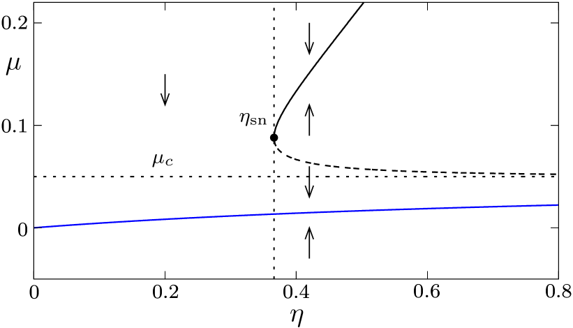
Figure 4: Fixed points of the slow dynamics (14) for varying control gain $\eta$. The values $\mu_{2,3}$ on the upper branch (black curve) correspond to periodic orbits of the layer equation (7), while $\mu_{1}$ (blue curve) is the branch of fixed points; solid and dashed lines indicate stable and unstable solutions, respectively. The direction of the motion in $\mu(T)$ is indicated by the arrows. The dotted lines indicate the onset of bistability for $\eta=\eta_{\textrm{sn}}$ and the transition at $\mu_{c}=1-I_{0}$ from equilibria to periodic orbits.

III Slow-fast analysis of the dynamics with noise

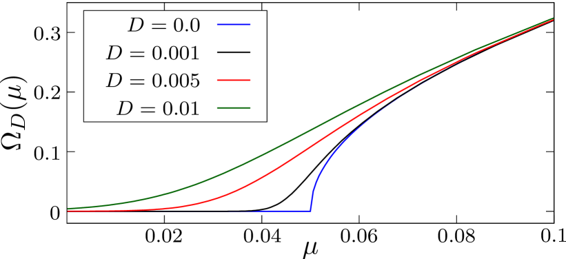
Figure 5: Average frequency of the fast dynamics (3) given by (26)- (27) using numerical solutions of the stationary Fokker-Planck equation (24), where $\mu$ acts as a time independent parameter and fixed $I_{0}=0.95$.

In this section, we consider the dynamics of system (3)–(4) in the presence of noise ($D>0$). In analogy to the noise-free case, one can use the limit $\varepsilon\rightarrow 0$ and employ the stochastic average

$$\langle\sin\varphi(t)\rangle_{t}=\lim_{t\longrightarrow\infty}\frac{1}{t}\int_{0}^{t}\sin\varphi(t)\mathrm{d}t^{\prime}$$

for solutions of the stochastic fast equation

$$\dot{\varphi}(t)=I_{0}+\mu-\sin\varphi(t)+\sqrt{D}\xi(t)$$ (22)

to approximate the slow dynamics in (11) by

$$\mu^{\prime}(T) =-\mu(T)+\eta(1-\langle\sin\varphi(t)\rangle_{t}).$$ (23)

To this end, we consider the stationary probability density distribution $\rho(\varphi;\mu,D)$ for the fast noisy dynamics (3), which for fixed control $\mu$ and noise intensity $D$ is given as a solution to the stationary Fokker-Planck equation

$$\frac{D}{2}\partial_{\varphi\varphi}\rho-\partial_{\varphi}\left[(I_{0}+\mu-\sin\varphi)\rho\right]=0,$$ (24)

together with the periodic boundary conditions $\rho(0)=\rho(2\pi)$ and the normalization

$$\int_{0}^{2\pi}\rho(\varphi;\mu,D)\mathrm{d}\varphi=1.$$ (25)

From this we can calculate the average

$$\langle\sin\varphi(t)\rangle_{t} =\int_{0}^{2\pi}\rho(\varphi;\mu,D)\sin\varphi\mathrm{d}\varphi$$ (26)

and obtain the mean frequency

$$\Omega_{D}(\mu) =I_{0}+\mu-\langle\sin\varphi(t)\rangle_{t},$$ (27)

which depends via (26) both on $D$ and $\mu$. Taking into account (23) and (27), the equation for the slow dynamics of $\mu(T)$ reads

$$\mu^{\prime}(T)=-\mu(T)+\eta(1-I_{0}-\mu+\Omega_{D}(\mu(T))),$$ (28)

i.e. it is of the same form as in the deterministic case (14). The corresponding fixed point equation for the stationary values of $\mu$ with respect to the slow dynamics is given by (18).

The stationary Fokker-Planck equation (24) can be solved directly by integral expressions, see Appendix B. In particular, for $D=0$ we readily recover the results for periodic averaging from the previous section. However, for small non-vanishing $D$, the integrals become difficult to evaluate numerically and we preferred to solve (24) as a first-order ODE boundary value problem with the software AUTO (Doedel et al., 2007), which provides numerical solutions to boundary value problems by collocation methods together with continuation tools for numerical bifurcation analysis.

In Fig. 5 are shown the numerically obtained effective frequencies $\Omega_{D}(\mu)$ for different noise levels $D$. Solving the stationary Fokker-Planck equation (24) together with the fixed point equation for $\mu(T)$ (18), we obtain for fixed values of $D$ and varying control gain $\eta$ branches of stationary solutions $(\mu^{\ast},\rho(\varphi;\mu^{\ast},D))$, see Fig. 6(a). For small noise intensities, these branches are folded, which indicates the coexistence of up to three stationary solutions, similar as in the noise-free case. Alternatively, we can also fix $\eta$ and obtain branches for varying $D$, see Fig. 7. For small $\eta$ they are monotonically increasing, while for larger $\eta$ they are folded. For $\eta_{\textrm{sn}}<\eta$ there are two separate branches, emanating from the three solutions of (18) at $D=0$.

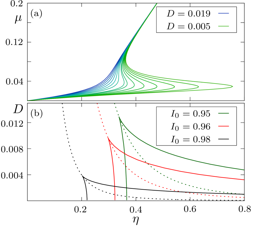
Figure 6: (a) Branches of fixed points $\mu^{\ast}(\eta)$ of the slow dynamics (28) for a set of noise values $D=0.005,0.006,\dots,0.019$, and $I_{0}=0.95$, calculated from (18) together with the stationary Fokker-Planck equation (24). (b) Two-dimensional bifurcation diagrams in terms of $\eta$ and $D$ for three different values of $I_{0}$ show the curves of fold bifurcations, which meet at the cusp point. Dashed curves indicate the case where $\mu=\mu_{c}=1-I_{0}$.

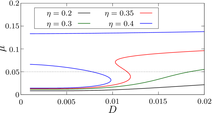
Figure 7: Branches of fixed points $\mu^{\ast}(D)$ of the slow dynamics (28) for a set of control gain values $\eta\in\left\{0.2,0.3,0.35,0.4\right\}$ and fixed $I_{0}=0.95$, calculated from (18) together with the stationary Fokker-Planck equation (24).

Continuation of the folds in the $(\eta,D)$ parameter plane provides the curves outlining the boundaries of the bistability region. Fig. 6(b) shows that the two branches of folds meet at the cusp point $(\eta_{\textrm{cu}},D_{\textrm{cu}})$. One of the branches approaches for $D\rightarrow 0$ the value $\eta=\eta_{\textrm{sn}}$, which we have calculated in (21), while the other one diverges to infinite values of $\eta$. When $I_{0}$ approaches the critical value $I_{0}=1,$ the cusp point shifts to a smaller noise intensity $D$, such that the region of bistability decreases.

Note that for $D>0$ all the average frequencies satisfy $\Omega_{D}>0$ such that a clear distinction between the stationary and the oscillatory regime of the fast dynamics is no longer possible. However, one can compare the critical value of the deterministic fast dynamics

$$\mu_{c}=1-I_{0}$$ (29)

with the corresponding stationary value $\mu^{*}$ of the slow variable from (28) to distinguish between a regime of noise-induced oscillations and oscillations derived from the deterministic part of the dynamics. If $\mu^{*}<\mu_{c}$, the oscillations are noise-induced and have the form of rare spikes, see Fig. 1(a),while for $\mu^{*}>\mu_{c}$ the deterministic oscillations are prevalent, see Fig. 1(c).

It turns out that the curves where the stationary values of $\mu$ satisfy the condition $\mu=\mu_{c}$, shown dashed in Fig. 6(b), pass exactly through the corresponding cusp point and inside the bistability region refer to the unstable solutions given by the middle part of the S-shaped curves in Fig. 6(a). From this we conclude that changing the parameters across this line outside the bistability region results in a gradual transition between the regimes of noise-induced oscillations and the deterministic-driven oscillations, while a hysteretic transition between the two stable regimes is obtained at the boundary of the bistability region. Moreover, for finite timescale separation $\varepsilon>0,$ there can be transitions between the two stable regimes also within the bistability region, which are induced by the stochastic fluctuations. In the following section we study in detail how the region of bistability found for the singular limit $\varepsilon\rightarrow 0$ also affects the dynamics of the original system in case of a finite timescale separation.

IV Effects of fluctuations and finite timescale separation

The two basic deterministic regimes of the fast dynamics, which are the excitable equilibrium and the oscillations, induce in a natural way the two corresponding states of the system with noise and small $\varepsilon>0$, namely

• Noise-induced spiking, characterized by a Poissonian-like distribution of inter-spike intervals (ISIs), see Fig. 8(a);

• Noisy oscillations, involving a Gaussian-like distribution of the ISIs, centered around the deterministic oscillation period, see Fig. 8(b).

These states are found for sufficiently small or large values of $\eta$, respectively, where only a corresponding single branch of the deterministic system is available and the fluctuations of $\mu$ around its average value have no substantial impact on the dynamics, cf. the blue and orange distributions in Fig. 8. For sufficiently large noise levels above the cusp $(D>D_{cu})$ and intermediate values of $\eta,$ one observes a gradual transition between these two regimes. However, for smaller noise $D<D_{cu}$, allowing for the existence of the region of bistability (cf. Fig. 6(b)), new regimes of stochastic dynamics can emerge, namely:

• Enhanced coherence resonance, where a noise-induced dynamical shift of the excitability parameter $I_{0}+\mu_{D}$ is self-adjusted close to criticality;

• Noise-induced switching between the two coexisting regimes in the bistability region, see Fig. 1(b).

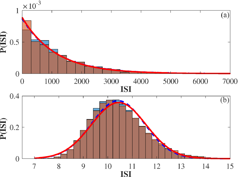
Figure 8: Histograms of inter spike intervals of the phase variable for control gain $\eta=0.2$ (top panel) and $\eta=0.5$ (bottom panel), obtained from numerical simulations of the full system (3)–(4) with $\varepsilon=0.005$ (orange) and in the limit of infinite timescale separation (blue), using (22) with the stationary $\mu(T)\equiv\mu_{D}$ determined from the stationary Fokker-Planck equation (24). Solid red and dashed blue curves represent fits to an exponential decay (a) and a Gaussian (b) for the histograms concerning the full system and the limit of infinite scale separation, respectively.

IV.1 Enhanced coherence resonance

The phenomenon of coherence resonance (Pikovsky and Kurths, 1997; Lindner and Schimansky-Geier, 1999; Makarov et al., 2001), where the regularity of noise-induced oscillations becomes maximal at an intermediate noise level, is well-known for noisy excitable systems such as the fast equation (22) without adaptation, i.e. for $\eta=0$ and therefore also $\mu=0$. For values of the control gain $0<\eta<\eta_{\textrm{cu}}$ below the region of bistability, the control leads to a substantially enhanced coherence resonance. This effect can be quantified by studying the noise dependence of the coefficient of variation of the inter spike intervals. For a given noisy trajectory of (22),the spiking times $t_{k}$ are defined as the first passage times $\varphi(t_{k})=2\pi k$, $k\in\mathbb{N}$ with corresponding inter spike intervals $\tau_{k}=t_{k}-t_{k-1}$. The coefficient of variation of their distribution is defined as

$$R(D) =\frac{\sqrt{\langle\tau_{k}^{2}\rangle-\langle\tau_{k}\rangle^{2}}}{\langle\tau_{k}\rangle}.$$ (30)

For (22) with a fixed $\mu$, the latter can be determined from direct numerical simulations. However, inserting for $\mu$ the corresponding stochastic averages $\mu^{*}(D;\eta)$ obtained in Section shows a strongly nonlinear dependence both on $\eta$ and $D$, see also Figs. 6(a) and 7. In particular, the strongly nonlinear dependence on $D$ for $\eta$ slightly below the cusp value $\eta_{\textrm{cu}}$ has a substantial impact on the resonant behavior reflected in the form of $R(D)$. In Fig. 9, we show the $R(D)$ dependence for different values of the control gain $\eta$, comparing the numerical results for the fast subsystem (22) with inserted stationary values $\mu^{*}(D;\eta)$, to numerical simulations of (3)-(4) for $\varepsilon=0.005$. While for $0<\eta<\eta_{cu}$ one finds that the coherence resonance can be substantially enhanced, cf. for example the $R(D)$ dependencies for $\eta=0$ and $\eta=0.3$, note that by introducing the negative values of the control gain $\eta,$ the resonant effect can be readily suppressed. This implies that the adaptive feedback we employ provides an efficient control of coherence resonance. Such an effect has already been demonstrated in (Aust et al., 2010; Kouvaris et al., 2010; Janson et al., 2004)by using a delayed feedback control of Pyragas type. However, this control method requires the feedback delay time as an additional control parameter to be well adapted to the maximum resonance frequency..

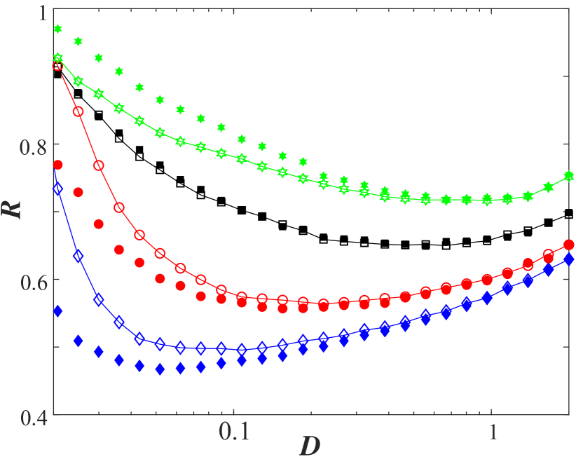
Figure 9: Enhancement or suppression of coherence resonance by a slowly adapting feedback control. The connected lines with empty symbols refer to $R(D)$ dependencies for the full system 3-4 at different values of the control gain: $\eta=-0.2$ (green hexagonals), $\eta=0$ (black squares), $\eta=0.2$ (red circles), and $\eta=0.3$ (blue diamonds), having fixed $I_{0}=0.95,\varepsilon=0.005$. The unconnected filled symbols indicate the corresponding $R(D)$ dependencies obtained from numerical simulations of the layer equation22 with stationary $\mu^{\ast}(D)$.

IV.2 Bursting behavior due to noise-induced switching

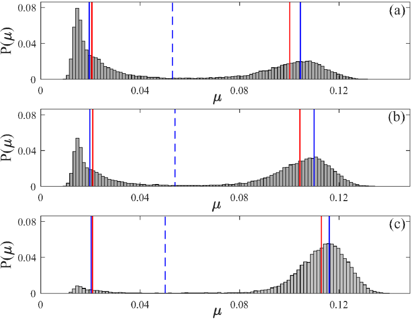
Figure 10: Stationary distributions $P(\mu)$, sampled from numerical simulations of (3)–(4) with $\varepsilon=0.005$. Parameters $\eta=0.37$ in (a), $\eta=0.373$ in (b) and $\eta=0.38$ in (c) and fixed noise level $D=0.009$ lie inside the bistability region from Fig. 6(b). Blue vertical lines indicate the fixed points of $\mu$ from the stationary Fokker-Planck equation (24) together with the fixed point equation (18) of the slow dynamics. Red vertical lines indicate the mean values of all $\mu$ in $P(\mu)$ below and of all $\mu$ above the unstable fixed point in the middle (dashed blue lines).

For parameter values $(\eta,D)$ within the bistable region and finite timescale separation $\varepsilon>0$, the coexisting states of excitable equilibrium and fast oscillations turn into metastable states of the full system (3)–(4). Based on our slow-fast analysis, the corresponding dynamics can be understood as follows. The noisy fluctuations of $\varphi(t)$ around its average distribution, given by the stationary Fokker-Planck equation (24), induces fluctuations of $\langle\sin{\varphi(t)}\rangle_{t}$, and hence also of $\mu$, around their stationary average values calculated above. For small $\varepsilon,$ the corresponding distribution of $\mu$ is centered in narrow peaks at the stable stationary values. However, with increasing $\varepsilon,$ the nonlinear filtering induces a strong skewness of each peak in the distribution, and their overlapping indicates the possibility of noise- induced transitions between the two metastable states. Figure 10 shows the distribution for $\varepsilon=0.005$ and different values of the $\eta$ within the bistability region. These transitions can be understood in analogy to the Eyring-Kramers process in a double well potential. In the generic case of different energy levels for the two potential wells, transitions in one of the directions occur at a higher rate and the system stays preferably in state associated to the global minimum of the potential. Such a behavior of biased switching is very pronounced closed to the boundaries of the bistability region, where a switching to the state close to the fold has a much lower probability than switching back.

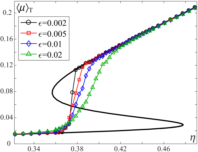
Figure 11: Long-time averages $\langle\mu\rangle_{T}$ from numerical simulations of (3), (4) with fixed noise intensity $D=0.008$ and varying control gain $\eta$ at different values of $\varepsilon\in\{0.002,0.005,0.01,0.02\}$. The black curve represents the corresponding result for the infinite timescale separation, cf. Fig. 6(a).

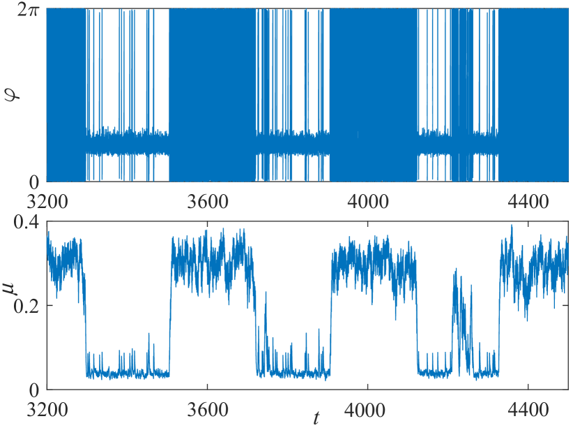
Figure 12: Time series $\varphi(t)$ (top panel) and $\mu(t)$ (bottom panel) illustrating the regime of balanced switching. The system parameters are $\eta=0.38,D=0.008,I_{0}=0.95,\varepsilon=0.01$.

In Fig. 11 are shown the numerical time averages $\langle\mu(T)\rangle$ for varying control gain $\eta$. One can see that for most values of $\eta$, the long time behavior is dominated by one of the two metastable states, which indicates a biased switching process. Nevertheless, at an intermediate value of $\eta,$ we find a balanced switching, where transitions in both directions occur at an almost equal rate. A corresponding time trace is shown in Fig. 12 and Fig. 1(b). For $\varepsilon\to 0,$ the switching rate decreases to zero exponentially and the switching bias in the unbalanced regime increases. This leads to the characteristic steplike behavior of the averages observed in Fig. 11 for smaller $\varepsilon$.

The noise-induced switching shown in Fig. 12 and Fig. 1(b) resembles the regime of bursting in neuronal systems. Here it emerges by an interplay of slow adaptation and noise. In the present setup, the bursts are triggered just by the stochastic fluctuations. However, in the regime $\eta>\eta_{\textrm{cu}},$ the system is also quite susceptible to external inputs, which could initiate the bursts even without any intrinsic noise.

V Discussion and outlook

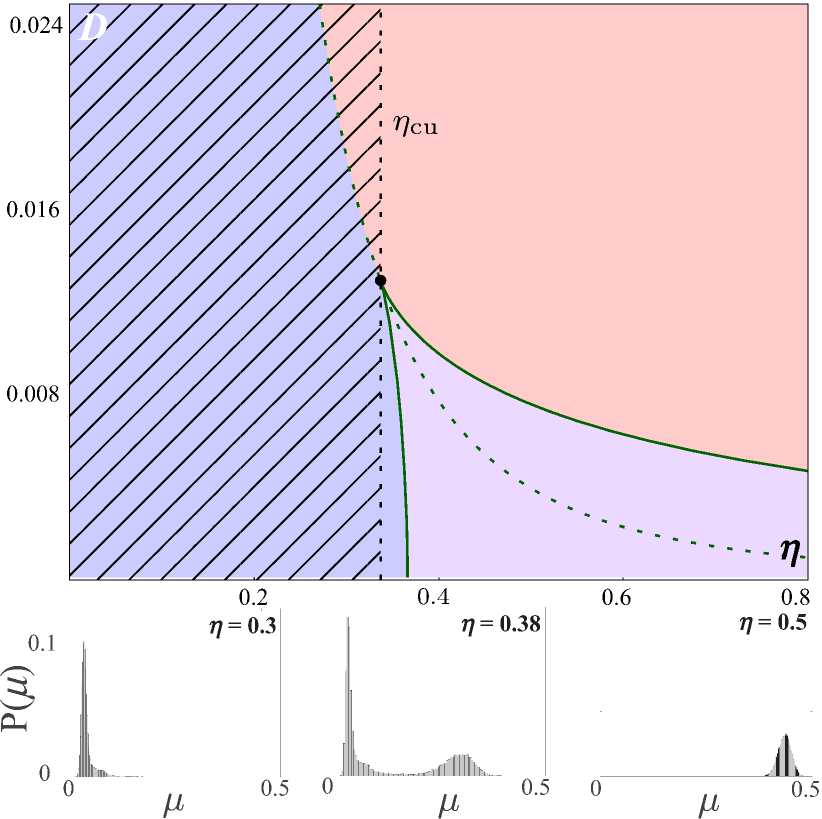
Figure 13: Upper panel: Parameter regions for different dynamical regimes: noise induced spiking (blue), noise perturbed oscillations (red), and noise induced bursting (violet). Enhanced coherence resonance can be found in the hatched region. Lower panels: Sampled distributions of $\mu(T)$ from numerical solutions with $\varepsilon=0.005,\,D=0.008$ and $\eta\in{0.3,0.38,0.5}$.

Our model provides a novel perspective on how the dynamics of an excitable system is influenced by the interaction of a slowly adapting feedback and noise. The feedback is taken from a low pass filter of a function that gives a positive feedback to the oscillations by pushing the excitability parameter towards the oscillatory regime. Since excitability, feedback, and noise are typical ingredients of neural systems, we believe that the application of our results to a specific neural model would be a next natural step, aiming to gain a deeper understanding of the onset of different dynamical regimes, as well as the means of controlling their properties and the emerging resonant effects. In Figure 13 are summarized our main results. In particular, the multiple timescale analysis for the limit of infinite timescale separation has allowed us to perform a numerical bifurcation analysis providing the parameter regions for the different dynamical regimes illustrated in Figure 1. Numerical simulations for finite values of $\varepsilon$ (lower panels in Fig. 13) show that the slowly varying control variable $\mu(T)$ is distributed around the stationary values from the limiting problem $\varepsilon=0$, see also Figure 10. Moreover, we have demonstrated that the filtered feedback in our model provides an efficient control of the effect of coherence resonance, which can be substantially enhanced or suppressed by a corresponding choice of the feedback gain. In the regime where the limiting problem $\varepsilon=0$ indicates a bistability between an equilibrium and a fast oscillation, the stochastic fluctuations at finite values of $\varepsilon$ give rise to a switching between the associated metastable states. However, our analysis shows that for sufficiently high noise intensity, this bistability vanishes and the two different deterministic states can no longer be distinguished.

From the point of view of the theory of multiscale systems, the deterministic part of the presented model provides one of the simplest examples combining the regimes of stable equilibrium and oscillations within the fast subsystem. A rigorous mathematical treatment of the dynamical transitions between the two regimes and the corresponding reductions by the standard adiabatic elimination and the averaging technique is still missing. Also, our approach to analysis of stochastic dynamics in multiscale systems by introducing a stationary Fokker-Planck equation for the fast dynamics leads to important questions concerning the limiting properties of the trajectories and the specific implications of the fluctuations. Nevertheless, we have considered only the case when the noise acts in the fast variable. An open problem is to study how the obtained results are influenced by the noise in the slow variable, where interesting new effects can be expected (Dannenberg et al., 2014).

Appendix A: Multiscale averaging in the regime of fast oscillations

In this appendix we provide a rigorous formal derivation of the slow averaged equation (14) for the case of periodic dynamics in the fast layers.

We apply the following general multiscale Ansatz

$$\varphi=\bar{\varphi}(t,\varepsilon t)+\varepsilon\hat{\varphi}(t,\varepsilon t),$$

$$\mu=\bar{\mu}(t,\varepsilon t)+\varepsilon\hat{\mu}(t,\varepsilon t).$$

Substituting this Ansatz into (3)–(4), one obtains up to the terms of the order $\varepsilon$

$$\partial_{1}\bar{\varphi}+\varepsilon\partial_{2}\bar{\varphi}+\varepsilon\partial_{1}\hat{\varphi} =I_{0}-\sin\left(\bar{\varphi}+\varepsilon\hat{\varphi}\right)+\bar{\mu}+\varepsilon\hat{\mu},$$

$$\partial_{1}\bar{\mu}+\varepsilon\partial_{2}\bar{\mu}+\varepsilon\partial_{1}\hat{\mu} =\varepsilon\left(-\bar{\mu}-\varepsilon\hat{\mu}+\eta\left(1-\sin\left(\bar{\varphi}+\varepsilon\hat{\varphi}\right)\right)\right),$$

where the subscripts 1 and 2 refer to partial derivatives with respect to $t$ and $\varepsilon t$, respectively. Collecting the terms of order $\mathcal{O}(1)$, one finds

$$\partial_{1}\bar{\varphi}=I_{0}-\sin\bar{\varphi}+\bar{\mu},$$ (31)

$$\partial_{1}\bar{\mu}=0.$$ (32)

The equation (32) implies that $\bar{\mu}=\bar{\mu}(\varepsilon t)$ depends only on the slow time and acts as a parameter in (31). For $\bar{\mu}>1-I_{0}$, equation (31) has the oscillating solution $\bar{\varphi}=\varphi_{\bar{\mu}}(t)$ given by (13). Note that the parameters of this solution can depend on the slow time.

As a next step, we consider the terms of order $\varepsilon$:

$$\partial_{2}\bar{\varphi}+\partial_{1}\hat{\varphi} =-\hat{\varphi}\cos\bar{\varphi}+\hat{\mu},$$

$$\partial_{2}\bar{\mu}+\partial_{1}\hat{\mu} =-\bar{\mu}+\eta\left(1-\sin\bar{\varphi}\right).$$ (33)

We rewrite Eq. (33) as

$$\partial_{2}\bar{\mu}+\bar{\mu}=-\partial_{1}\hat{\mu}+\eta\left(1-\sin\bar{\varphi}\right),$$ (34)

where the left-hand side depends only on the slow time. Hence, the solvability condition for (34) is the requirement that its right-hand side is independent on the fast time $t$, i.e.

$$-\partial_{1}\hat{\mu}+\eta\left(1-\sin\bar{\varphi}\right)=u(T)$$ (35)

with some function $u(T),$where $T=\varepsilon t$ is the slow time. By integrating (35) with respect to the fast time, we obtain

$$\hat{\mu}(t)=\hat{\mu}(0)+\eta\left(t-\int_{0}^{t}\sin\bar{\varphi}dt\right)-tu(T)$$ (36)

The integral in (36) can be computed using (31):

$$\int_{0}^{t}\sin\bar{\varphi}dt=tI_{0}+t\bar{\mu}-\bar{\varphi}(t)+\bar{\varphi}(0)$$

such that

$$\hat{\mu}(t)=\hat{\mu}(0)+t\left[\eta\left(1-I_{0}-\bar{\mu}+\frac{\bar{\varphi}(t)-\bar{\varphi}(0)}{t}\right)-u(T)\right]$$

Taking into account that

$$\frac{\bar{\varphi}(t)-\bar{\varphi}(0)}{t}=\Omega(\bar{\mu})+\mathcal{O}\left(\frac{1}{t}\right),$$

we obtain the expression for $\hat{\mu:}$

$$\hat{\mu}(t)=\hat{\mu}(0)+t\left[\eta\left(1-I_{0}-\bar{\mu}+\Omega(\bar{\mu})\right)-u(T)\right]+\mathcal{O}(1),$$

where the linearly growing term must vanish for $\hat{\mu}(t)$ to be bounded. Setting such a secular term to zero (even without computing explicitly $\hat{\mu}$), we have

$$u(T)=\eta\left(1-I_{0}-\bar{\mu}+\Omega(\bar{\mu})\right),$$

and, hence, taking into account (34) and (35), the equation for the leading order approximation of the slow variable reads

$$\partial_{2}\bar{\mu}+\bar{\mu}=\eta\left(1-I_{0}-\bar{\mu}+\Omega(\bar{\mu})\right).$$

Since $\bar{\mu}$ is the function of the slow time only, we have $\partial_{2}\bar{\mu}=\bar{\mu}^{\prime}$ ,which results in the required averaged equation (14).

Appendix B: Explicit solution of the stationary Fokker-Planck equation

Here we present the analytic solution of the stationary Fokker-Planck equation (24)–(25). By integrating Eq. (24) once one obtains

$$\frac{D}{2}\partial_{\varphi}\rho-\left(I_{0}+\mu-\sin\varphi\right)\rho=C$$ (37)

with a constant $C$ to be determined. Solving (37), and taking into account the normalization (25) and the boundary condition $\rho(0)=\rho(2\pi)$, we arrive at

$$\rho(\varphi;\mu,D)=\frac{1}{g_{\Lambda}}\Lambda(\varphi),$$

where

$$\Lambda(\varphi)=\int_{0}^{2\pi}\frac{\Psi(\varphi)}{\Psi(\varphi+\xi)}d\xi,$$

$$g_{\Lambda}=\int_{0}^{2\pi}\Lambda(\varphi)d\xi,$$

$$\Psi(\varphi)=\exp\left\{\frac{2}{D}\left[(I_{0}+\mu)\varphi+\cos\varphi-1\right]\right\}.$$

References

- Izhikevich (2007) E. M. Izhikevich, Dynamical Systems in Neuroscience: The Geometry of Excitability and Bursting (The MIT Press, 2007), ISBN 9780262090438, URL https://mitpress.mit.edu/books/dynamical-systems-neuroscience.
- Gerstner et al. (2014) W. Gerstner, W. M. Kistler, R. Naud, and L. Paninski, Neuronal dynamics: From single neurons to networks and models of cognition (2014), ISBN 9781107447615, URL https://doi.org/10.1017/CBO9781107447615.
- Abbott and Dayan (2005) L. F. Abbott and P. Dayan, Theoretical Neuroscience (The MIT Press, 2005), URL https://mitpress.mit.edu/books/theoretical-neuroscience.
- Clopath et al. (2010) C. Clopath, L. Büsing, E. Vasilaki, and W. Gerstner, Nat. Neurosci. 13, 344 (2010), URL https://doi.org/10.1038/nn.2479.
- Popovych et al. (2013) O. Popovych, S. Yanchuk, and P. A. P. Tass, Sci. Rep. 3, 2926 (2013), URL https://doi.org/10.1038/srep02926.
- Lang and Kobayashi (1980) R. Lang and K. Kobayashi, IEEE J. Quantum Electron. 16, 347 (1980), URL https://doi.org/10.1109/JQE.1980.1070479.
- Lüdge (2011) K. Lüdge, Nonlinear Laser Dynamics (Wiley-VCH Verlag GmbH & Co. KGaA, Weinheim, Germany, 2011), ISBN 9783527639823, URL http://doi.wiley.com/10.1002/9783527639823.
- Soriano et al. (2013) M. C. Soriano, J. García-Ojalvo, C. R. Mirasso, and I. Fischer, Rev. Mod. Phys. 85, 421 (2013), URL https://doi.org/10.1103/RevModPhys.85.421.
- Krupa et al. (1997) M. Krupa, B. Sandstede, and P. Szmolyan, J. Differ. Equ. 133, 49 (1997), URL https://doi.org/10.1006/jdeq.1996.3198.
- Lichtner et al. (2011) M. Lichtner, M. Wolfrum, and S. Yanchuk, SIAM J. Math. Anal. 43, 788 (2011), URL https://doi.org/10.1137/090766796.
- Desroches et al. (2012) M. Desroches, J. Guckenheimer, B. Krauskopf, C. Kuehn, H. M. Osinga, and M. Wechselberger, SIAM Rev. 54, 211 (2012), URL http://epubs.siam.org/doi/10.1137/100791233.
- Kuehn (2015) C. Kuehn, Multiple Time Scale Dynamics, vol. 191 (Springer-Verlag GmbH, 2015), ISBN 978-3-319-12315-8, URL http://link.springer.com/10.1007/978-3-319-12316-5.
- Jardon-Kojakhmetov and Kuehn (2019) H. Jardon-Kojakhmetov and C. Kuehn (2019), eprint 1901.01402, URL http://arxiv.org/abs/1901.01402.
- Haken (1985) H. Haken, Advanced Synergetics (Springer Berlin Heidelberg, 1985), URL https://link.springer.com/book/10.1007/978-3-642-45553-7.
- Lindner et al. (2004) B. Lindner, J. García-Ojalvo, A. Neiman, and L. Schimansky-Geier, Phys. Rep. 392, 321 (2004), URL https://linkinghub.elsevier.com/retrieve/pii/S0370157303004228.
- Destexhe and Rudolph-Lilith (2012) A. Destexhe and M. Rudolph-Lilith, Neuronal Noise (Springer New York, 2012), URL https://www.springer.com/gp/book/9780387790190.
- Forgoston and Moore (2018) E. Forgoston and R. O. Moore, SIAM Rev. 60, 969 (2018), URL https://doi.org/10.1137/17M1142028.
- Murray (1989) J. D. Murray, Mathematical Biology, vol. 19 of Biomathematics (Springer, New York, 1989), ISBN 0-387-19460-6 (New York), 3-540-19460-6 (Berlin), URL https://www.springer.com/gp/book/9780387952239.
- Winfree (2001) A. T. Winfree, The Geometry of Biological Time, vol. 12 (Springer, 2001), ISBN 978-1-4419-3196-2, URL http://link.springer.com/10.1007/978-1-4757-3484-3.
- Pikovsky and Kurths (1997) A. S. Pikovsky and J. Kurths, Phys. Rev. Lett. 78, 775 (1997), URL https://doi.org/10.1103/PhysRevLett.78.775.
- Oriol et al. (2011) V.-C. Oriol, M. Ronny, R. Sten, and L. Schimansky-Geier, Phys. Rev. E 83, 036209 (2011), URL https://doi.org/10.1103/PhysRevE.83.036209.
- Ermentrout and Kleinfeld (2001) G. B. Ermentrout and D. Kleinfeld, Neuron 29, 33 (2001), URL https://doi.org/10.1016/S0896-6273(01)00178-7.
- Lücken et al. (2017) L. Lücken, D. P. Rosin, V. M. Worlitzer, and S. Yanchuk, Chaos 27, 13114 (2017), URL http://aip.scitation.org/doi/full/10.1063/1.4971971.
- Franović et al. (2018) I. Franović, O. E. Omel’chenko, and M. Wolfrum, Chaos 28, 071105 (2018), URL https://aip.scitation.org/doi/10.1063/1.5045179.
- Bačić et al. (2018) I. Bačić, S. Yanchuk, M. Wolfrum, and I. Franović, EPJ ST 227, 1077 (2018), URL https://link.springer.com/article/10.1140/epjst/e2018-800084-6.
- Franović et al. (2015a) I. Franović, K. Todorović, M. Perc, N. Vasović, and N. Burić, Phys. Rev. E 92, 062911 (2015a), URL https://doi.org/10.1103/PhysRevE.92.062911.
- Franović et al. (2015b) I. Franović, M. Perc, K. Todorović, S. Kostić, and N. Burić, Phys. Rev. E 92, 062912 (2015b), URL https://doi.org/10.1103/PhysRevE.92.062912.
- Yanchuk et al. (2019) S. Yanchuk, S. Ruschel, J. Sieber, and M. Wolfrum, Phys. Rev. Lett. 123, 053901 (2019), URL https://doi.org/10.1103/PhysRevLett.123.053901.
- Izhikevich (2004) E. M. Izhikevich, IEEE Trans. Neural Netw. 15, 1063 (2004), URL https://doi.org/10.1109/TNN.2004.832719.
- Strogatz (1994) S. H. Strogatz, Nonlinear Dynamics and Chaos: with Applications to Physics, Biology, Chemistry, and Engineering (Addison-Wesley, 1994), URL https://www.crcpress.com/Nonlinear-Dynamics-and-Chaos-With-Applications-to-Physics-Biology-Chemistry/Strogatz/p/book/9780813349107.
- Shilnikov and Kolomiets (2008) A. Shilnikov and M. Kolomiets, Int. J. Bifurc. Chaos 18, 2141 (2008), URL https://doi.org/10.1142/S0218127408021634.
- Pavliotis and Stuart (2008) G. Pavliotis and A. Stuart, Multiscale Methods: Averaging and Homogenization (Springer Berlin Heidelberg, 2008), URL https://www.springer.com/gp/book/9780387738284.
- Galtier and Wainrib (2012) M. Galtier and G. Wainrib, Phys. Rev. E 2, 13 (2012), URL https://doi.org/10.1186/2190-8567-2-13.
- Lücken et al. (2016) L. Lücken, O. V. Popovych, P. A. Tass, and S. Yanchuk, Phys. Rev. E 93, 32210 (2016), URL https://doi.org/10.1103/PhysRevE.93.032210.
- Doedel et al. (2007) E. J. Doedel, R. C. Paffenroth, A. R. Champneys, T. F. Fairgrieve, Y. A. Kuznetsov, B. Sandstede, and X. Wang, AUTO-07p: Continuation and bifurcation software for ordinary differential equations (Montreal, Canada, 2007), URL http://indy.cs.concordia.ca/auto/.
- Lindner and Schimansky-Geier (1999) B. Lindner and L. Schimansky-Geier, Phys. Rev. E 60, 7270 (1999), URL https://doi.org/10.1103/PhysRevE.60.7270.
- Makarov et al. (2001) V. A. Makarov, V. I. Nekorkin, and M. G. Velarde, Phys. Rev. Lett. 86, 3431 (2001), URL https://doi.org/10.1103/PhysRevLett.86.3431.
- Aust et al. (2010) R. Aust, P. Hövel, J. Hizanidis, and E. Schöll, Eur. Phys. J. Spec. Top. 187, 77 (2010), URL https://link.springer.com/article/10.1140/epjst/e2010-01272-5.
- Kouvaris et al. (2010) N. Kouvaris, L. Schimansky-Geier, and E. Schöll, Eur. Phys. J. Spec. Top. 191, 29 (2010), URL https://link.springer.com/article/10.1140/epjst/e2010-01340-x.
- Janson et al. (2004) N. B. Janson, A. G. Balanov, and E. Schöll, Phys. Rev. Lett. 93, 010601 (2004), URL https://journals.aps.org/prl/abstract/10.1103/PhysRevLett.93.010601.
- Dannenberg et al. (2014) P. H. Dannenberg, J. C. Neu, and S. W. Teitsworth, Phys. Rev. Lett. 113, 020601 (2014), URL https://doi.org/10.1103/PhysRevLett.113.020601.