Bound states in ultrastrong waveguide QED

Abstract

We discuss the properties of bound states in finite-bandwidth waveguide QED beyond the Rotating Wave Approximation or excitation number conserving light-matter coupling models. Therefore, we extend the standard calculations to a broader range of light-matter strengths, in particular, in the so-called ultrastrong coupling regime. We do this using the Polaron technique. Our main results are as follows. We compute the spontaneous emission rate, which is renormalized as compared to the Fermi Golden Rule formula. We generalise the existence criteria for bound states, their properties and their role in the qubits thermalization. We discuss effective spin-spin interactions through both vacuum fluctuations and bound states. Finally, we sketch a perfect state-transfer protocol among distant emitters.

I Introduction

Photons are weakly coupled to matter, so they rarely interact, making them perfect information carriers. Weak coupling constitutes, however, a double-edged sword, as it also hinders the readout process when the time comes to access the information being carried. The trade off is optimized in waveguide QED, where the photons are confined in one dimensional waveguides to enhance the light-matter coupling Roy et al. (2017); Gu et al. (2017). So far, different experimental platforms have been used to implement this coupling between quantum emitters (typically two level systems or qubits) and a one dimensional quantized electromagnetic field. Examples are superconducting circuits Astafiev et al. (2010); Van Loo et al. (2013); Liu and Houck (2017), optical waveguides Faez et al. (2014) among others Lodahl et al. (2015); Chang et al. (2018). Waveguide QED can serve to control light-matter emission, to induce photon-photon interactions or to route the photons in quantum networks. Besides, by engineering the guides, more exotic interfaces can be implemented for quantum simulation Argüello-Luengo et al. (2019), topological photonics Bello et al. (2019), chirality Lodahl et al. (2017); Sánchez-Burillo et al. (2019a) or quantum computing Zheng et al. (2013). Consequently, waveguide QED may be a quantum technological solution.

Trying to optimize the light-matter coupling, several experiments have reached the so-called ultrastrong coupling regime (USC) between light and a single quantum emitter, both in cavity Niemczyk et al. (2010); Forn-Díaz et al. (2010) and waveguide QED Forn-Díaz et al. (2017); Martínez et al. (2019); Leger et al. (2019). The USC is the regime where higher order processes, than the creation (annihilation) of one photon by annihilating (creating) one matter excitation play a role. Two main phenomena are paradigmatic of USC. The Rotating Wave Approximation (RWA) for the interaction breaks down and the atomic bare parameters get renormalized, either the Bloch-Siegert shift Shirley (1965) in cavity QED or the renormalization due to the coupling to the continuum electromagnetic (EM) field in waveguide QED Leggett et al. (1987). Besides, the ground state becomes nontrivial Ashhab and Nori (2010). This has interesting consequences. Some of them are the possibility of transforming virtual onto real photons by perturbing the ground state Ciuti et al. (2005); Stassi et al. (2013); He et al. (2018); Liberato (2017), doing nonlinear optics with zero photons Stassi et al. (2017). Further phenomenology in cavity QED can be found in recent reviews Kockum et al. (2019); Forn-Díaz et al. (2019). In this work we are interested in the USC regime in waveguide QED. Apart from the qubit frequency renormalization, there exist the localization-delocalization transition Peropadre et al. (2013); Shi et al. (2018a), particle production Gheeraert et al. (2018), non-linear optics at the single photon limit Sánchez-Burillo et al. (2014, 2015) or vacuum light emission Sánchez-Burillo et al. (2019b).

In conventional waveguide QED, i.e. when the RWA can be performed, the main objective is to control atom-atom interactions mediated by the waveguide’s EM-fluctuations Dzsotjan et al. (2011); Gonzalez-Tudela et al. (2011); Zueco et al. (2012); Zheng and Baranger (2013); Manzoni et al. (2017). Propagating photons induce long range but dissipative interactions. Dissipative because the information is lost in the travelling wavepackets. On the other hand, dressed atom-field eigenstates localized around the quantum emitter, called bound states John (1984, 1987); John and Wang (1990, 1991); John and Quang (1994), generate non dissipative but exponentially-bounded interactions González-Tudela et al. (2015); Douglas et al. (2015); Shi et al. (2016); Calajó et al. (2016); González-Tudela and Cirac (2017a, b, 2018, 2018); González-Tudela and Galve (2018); Shi et al. (2018b); Bello et al. (2019); Sánchez-Burillo et al. (2019a). These exact non-propagating eigenstates lie within the band gap (hence non-propagating). Besides, bound states modify the spontaneous emission Khalfin (1958); Bykov (1975); Fonda et al. (1978); Onley and Kumar (1992); Gaveau and Schulman (1995); Garmon et al. (2009, 2013); Garmon (2013); Lombardo et al. (2014); Sánchez-Burillo et al. (2017) which makes them an interesting resource for engineering quantum photonics.

In this work, we discuss the physics of bound states in the USC regime of waveguide QED. We focus on the lowest energy ones, discussing their existence and role in the spontaneous emission and thermalization. We also discuss the effective spin-spin models emerging when several emitters are ultrastrongly coupled to the EM field and envision protocols for perfect state transfer between distant atoms. To do this, we face a technical difficulty. The light-matter coupling is modelled via spin(s)-boson type Hamiltonians, a paradigmatic example of a non exactly solvable model Ulrich (1999). Different techniques are available in the literature to deal with it. Matrix-product states (MPS) Peropadre et al. (2013); Sánchez-Burillo et al. (2014, 2015) , density matrix renormalization group (DMRG) Prior et al. (2010) or path integral approaches Grifoni and Hänggi (1998); Le Hur (2010), comprise the toolbox of numerical techniques. Analytical treatments are also used. They are based on different varational anstatzs: Polaron-like Silbey and Harris (1984); Bera et al. (2014); Díaz-Camacho et al. (2016); Shi et al. (2018a); Zueco and García-Ripoll (2019); Sánchez-Burillo et al. (2019b) or Gaussian ones Shi et al. (2018c). In this manuscript we will use a Polaron-type approach that has been shown to be accurate in a wide range of parameters, including couplings well inside the USC.

The rest of the manuscript is organized as follows. In the next section, Sect. II, we will introduce the system, its model and the Polaron picture. In Section III, we treat the single emitter case. We discuss the ground state properties and the lowest bound state, discussing its existence conditions, energy, and localization length. Section IV develops the multiqubit case with emphasis in the effective tight-binding model and in protocols for perfect state transfer. We finish with some conclusions. Several technical issues are sent to the appendices. Finally, the link to the python codes used in the numerical calculations is given in App. D.

II Light-matter interaction and the Polaron picture

II.1 Model

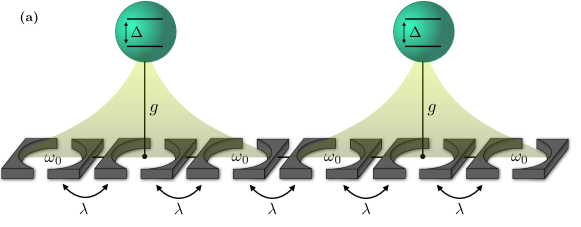
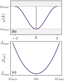
Figure 1: (a) Schematic depiction of two qubits coupled to specific sites of a linear cavity array. Where $g$ is the coupling constant, $\Delta$ is the energy difference between the two states of the qubits, $\omega_{0}$ is the resonance frequency for photons in the cavity (omitted in the coupled cavities for aesthetic purposes) and $\lambda$ is the hopping constant for photons travelling between cavities. The yellow shades represent localized-photon clouds. (b) Finite-band dispersion relation of the model. (c) Spectral density function for the model.

In this manuscript we study the system sketched in Fig. 1(a). Several qubits are coupled to a cavity array forming the photonic medium. In the dipole gauge Di Stefano et al. (2019) and assuming that each qubit is coupled to a single cavity, the model is ($\hbar=1$ is set through the paper)

$$H =\sum_{j=1}^{N_{q}}\frac{\Delta}{2}\sigma_{j}^{z}+\omega_{0}\sum_{n}^{N}b_{n}^{\dagger}b_{n}-\lambda\sum_{n}^{N}\left(b^{\dagger}_{n}b_{n-1}+{\rm H.c.}\right)$$

$$+g\sum_{j=1}^{N_{q}}\sigma_{j}^{x}\left(b_{x_{j}}^{\dagger}+b_{x_{j}}\right)\;.$$ (1)

Here, $N_{q}$ is the total number of qubits with level splitting $\Delta$ (let us assume that all the atoms are identical). $N$ is the number of sites; we will consider the thermodynamic limit $N\to\infty$ in our analytical treatment. $x_{j}$ is the site to which the $j$th-qubit is coupled. Operators $b_{n}^{\dagger}$ and $b_{n}$ correspond to the bosonic creation and annihilation operators at site $n$, and $\sigma^{z}$ and $\sigma^{x}$ are the $z$ and $x$ Pauli matrices. To avoid extra parameters, we will consider that the qubit-resonator coupling is the same for all the qubits, $g$. The photonic medium (second and third term in Eq. (II.1)), which is a cavity array, is diagonalized introducing the bosonic operators in momentum space, which are the Fourier transform of their spatial counterparts: $b_{k}=\frac{1}{\sqrt{N}}\sum_{n}e^{ikn}b_{n}$ obtaining:

$$H =\frac{\Delta}{2}\sum_{j=1}^{N_{q}}\sigma_{j}^{z}+\sum_{k}\omega_{k}b_{k}^{\dagger}b_{k}$$

$$+\sum_{j=1}^{N_{q}}\sigma_{j}^{x}\sum_{k}c_{k}\left(b_{k}^{\dagger}e^{ikx_{j}}+b_{k}e^{-ikx_{j}}\right).$$ (2)

The dispersion relation, sketched in Fig. 1(b), is

$$\omega_{k}=\omega_{0}-2\lambda\cos k,$$ (3)

and the coupling per spin in momentum space is given by

$$c_{k}=\frac{g}{\sqrt{N}}.$$ (4)

The dispersion relation is a finite band of width $4\lambda$ centred around $\omega_{0}$. Besides, the coupling constant is independent of the photonic mode and proportional to $g$, which justifies why, through out this work, we refer to both $g$ and $c_{k}$ indistinctly as the coupling constant. Finally, it is convenient to define the spectral density, plotted in Fig. 1(c),

$$J(\omega)=2\pi\sum_{k}|c_{k}|^{2}\delta(\omega-\omega_{k})\;,$$ (5)

conveniently rewritten in terms of the density of states

$$J(\omega)=2\pi g^{2}\left(\frac{d\omega_{k}}{dk}\right)^{-1}\;.$$ (6)

II.2 A brief comment on the RWA

If the coupling constant is small enough, the Rotating Wave Approximation can be used, by which the interaction term [last term in Eq. (II.1)] becomes

$$\sum_{j=1}^{N_{q}}\sum_{k}c_{k}\left(\sigma_{j}^{-}b_{k}^{\dagger}+\sigma_{j}^{+}b_{k}\right).$$ (7)

It is clear now that the state $\ket{0_{1},0_{2},\dots,0_{N_{q}};{\bf 0}}$ with $\sigma^{z}_{j}|0_{j}\rangle=-|0_{j}\rangle$ and $b_{k}|{\bf 0}\rangle=0$ is the (trivial) ground state (GS) of the system and that the Hamiltonian preserves the number of excitations $N$, $\left[H,N\right]=0$ with $N=\sum_{k}b_{k}^{\dagger}b_{k}+\sum_{j=1}^{N_{q}}\sigma_{j}^{+}\sigma_{j}^{-}$. Consequently, within the RWA, the dynamics are split in subspaces with a fixed number of excitations which makes the low-energy dynamics amenable, at least numerically.

II.3 Polaron picture

It has been shown that in the low-energy sector of a spin(s)-boson model [(2)] is well approximated by an effective, excitation-number-conserving Hamiltonian derived from a Polaron transformation Bera et al. (2014); Díaz-Camacho et al. (2016). The basic idea is to construct a unitary transformation that disentangles the TLS from the bath. This unitary transformation depends on some parameters that are found with the variational principle. In this case, the ansatz is,

$$|\Psi_{GS}[f_{k},c_{\bf s}]\rangle=U_{P}[f_{k}]\;|{\bf 0}\rangle\otimes\sum_{s_{j}=0,1}c_{\bf s}|s_{1},...,s_{N_{p}}\rangle\;.$$ (8)

Here $|{\bf 0}\rangle$ is the photon vacuum state ($b_{k}|{\bf 0}\rangle=0$ for all $k$) and the spin state is arbitrary. The varational parameters are the $c_{\bf s}$-coefficients and $\{f_{k}\}$, the $N$ parameters in the unitary $U_{P}$. Building up on previous work from McCutcheon et al. McCutcheon et al. (2010) and Zheng et al. Zheng et al. (2015) we used a natural extension of the single-qubit Polaron transform valid for arbitrarily distant qubits

$$U_{P}=\exp[-\sum_{j=1}^{N_{q}}\sigma_{j}^{x}\sum_{k}(f_{k}b_{k}^{\dagger}e^{ikx_{j}}-f_{k}^{*}b_{k}e^{-ikx_{j}})].$$ (9)

Provided there is no privileged direction of travel, we can assume that for each boson with wavenumber $k$ there will be another with $-k$, so that $|f_{k}|=|f_{-k}|$. From that, and the fact that the sine is odd, Eq. (9) factors as

$$U_{P}=\bigotimes_{j=1}^{N_{q}}\;U_{j}\;,$$ (10)

with

$$U_{j}=\exp[-\sigma_{j}^{x}\sum_{k}(f_{k}b_{k}^{\dagger}e^{ikx_{j}}-f_{k}^{*}b_{k}e^{-ikx_{j}})].$$

It turns out that minimizing the energy of the spins-boson [(2)],

$$\epsilon_{GS}={\rm min}_{f_{k},c_{\bf s}}\{\langle\Psi_{GS}[f_{k},c_{\bf s}]|H|\Psi_{GS}[f_{k},c_{\bf s}]\rangle\}$$ (11)

is done by finding the ground state of the effective spin model

$${\mathcal{H}}_{S}=\frac{\Delta_{r}}{2}\sum_{j=1}^{N_{q}}\sigma^{z}_{j}+\sum_{i<j}\mathcal{J}_{ij}\sigma_{i}^{x}\sigma_{j}^{x}+N_{q}\sum_{k}f_{k}(w_{k}f_{k}-2c_{k})$$ (12)

with

$$\mathcal{J}_{ij}=2\sum_{k}f_{k}(2c_{k}-\omega_{k}f_{k})\cos[k(x_{i}-x_{j})]\;,$$ (13)

and the renormalized qubits frequency

$$\Delta_{r}=\Delta\exp[-2\sum_{k}|f_{k}|^{2}]\;.$$ (14)

In the next section we will work explicit expressions in the case of one and two qubits. A generalized Polaron transformation is discussed in App. C, where it is shown that the much less cumbersome Eq. (9) is sufficiently good.

III Single qubit case

In the single qubit case, $N_{q}=1$, Hamiltonian [(2)] is nothing but the spin-boson model Leggett et al. (1987) (Ulrich, 1999, Chap. 3). In this section, we tackle the ground-state properties, the single-qubit bound states, and the spontaneous emission within the USC regime for the cavity array model [Eq. (6)].

III.1 Ground state

Setting $N_{q}=1$, Eqs. (11) and (12) yield that the minimum of the energy is reached when $\sigma_{z}|s_{1}\rangle=-|s_{1}\rangle$ [Cf. (12)] with

$$\bar{E}_{GS}=-\frac{\Delta_{r}}{2}+\sum_{k}w_{k}|f_{k}|^{2}-\sum_{k}c_{k}\left(f_{k}+f_{k}^{*}\right),$$ (15)

which is minimum when Silbey and Harris (1984),

$$f_{k}=\frac{c_{k}}{\Delta_{r}+\omega_{k}}.$$ (16)

Putting together Eqs. (14) and (16), we realize that the qubit frequency renormalizes to zero as the coupling strength increases. This is a well known result Leggett et al. (1987). Besides, this renormalization is the responsible for the localization-delocalization phase transition that corresponds to the ferromagnetic-antiferromagnetic phase transition in the Kondo model Guinea et al. (1998). The delocalized phase corresponds to $\Delta_{r}\to 0$, then the qubit state can be in either the symmetric or antisymmetric superpositions of the eigenstates of $\sigma^{z}$. On the other hand, if $c_{k}=0$, the spin is at an eigenstate of $\sigma_{z}$, which corresponds to the localized sector . Using Eqs. (5) and (16) we can rewrite Eq. (14) as,

$$\Delta_{r}=\Delta\exp{-\frac{1}{\pi}\int d\omega\frac{J(\omega)}{(\Delta_{r}+\omega)^{2}}}\;.$$ (17)

Having a phase transition depends on $J(\omega)$ Spohn1 and Domcke1 (1985). In our system it is not expected to have critical behaviour Löwen (1988). It is not within the aspirations of this work to study (the absence of) this phase transition, partly because it is not clear that the PT is valid in these ranges, so we will restrict our study to the so-called ultra-strong coupling region, $g\in(0,\sim 0.5)$, where we are confident that the Polaron ansatz works Zueco and García-Ripoll (2019); Sánchez-Burillo et al. (2019b). As we can see from Fig. 2(a), this region is characterized by a significant, albeit not complete, shrinkage of the tunneling frequency ($\Delta$), and as such we expect predictions from RWA to fail.

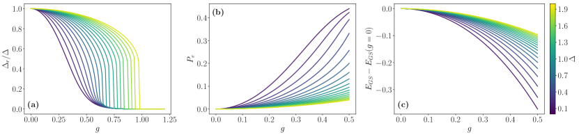
Figure 2: (a) Renormalized frequency in units of the bare qubit frequency as a function of $g$ for several values of $\Delta$. (b) $P_{e}$ as a function of $g$ for several values of $\Delta$. (c) Dependence of the ground state energy with $g$ for several values of $\Delta$, plotted with respect to the GS energy of an uncoupled qubit and the bath.

We can further characterize the GS by computing spin observables as is $P_{e}=\expectationvalue{\sigma^{+}\sigma^{-}}$, the probability of having the spin excited. This is an insightful observable because it relates a measurable quantity, $P_{e}$, to the renormalized frequency, $\Delta_{r}$:

$$P_{e}=\expectationvalue{\sigma^{+}\sigma^{-}}{GS}=\frac{1}{2}\left(1-\frac{\Delta_{r}}{\Delta}\right).$$ (18)

Here we used $\sigma^{+}\sigma^{-}=\frac{1}{2}(\sigma^{z}+I)$ together with $\expectationvalue{\sigma^{z}}{GS}=\expectationvalue{U_{P}^{\dagger}\sigma^{z}U_{P}}{0}=-\frac{\Delta_{r}}{\Delta}$. In Fig. 2(b) we show the dependence of $P_{e}$ with $\Delta$ and $g$, alongside is the GS energy plotted in the same parameter range, in Fig. 2(c). These are signatures of RWA failure, since within the RWA both $P_{e}$ and $E_{GS}$ are zero.

Another interesting observable is the spatial distribution of the photons, $\expectationvalue{b_{n}^{\dagger}b_{n}}$. Some algebra (fully done in App. A.2) yields

$$\expectationvalue{b_{n}^{\dagger}b_{n}}=f_{n}^{2}$$ (19)

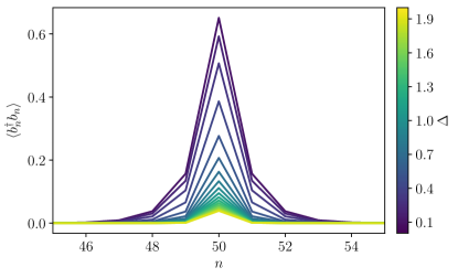
Figure 4: Comparison of the spatial distribution of GS photons for $g=0.5$.

with $f_{n}=\frac{1}{\sqrt{N}}\sum_{k}e^{ik(n-N/2)}f_{k}$ being the Fourier transform of $f_{k}$. We center the transformation at the qubit position that it is understood to be at the middle of the chain. Notice that $f_{n}$ has the clear interpretation of being the real-space variational amplitudes for the Polaron transformation. Figure 4 shows the spatial distribution of photons as calculated in Eq. (19). We observe that they are well localized around the impurity, exhibiting exponential decay $f_{n}\sim\exp\{-\kappa_{GS}(n-N/2)\}$ with localization lenght (See App. A.3 for a proof)

$$\kappa_{GS}^{-1}=\text{arccosh}^{-1}\left(\frac{\omega_{0}+\Delta_{r}}{2\lambda}\right).$$ (20)

The photons dressing the impurity are commonly named virtual photons in reference to their special properties of being non-propagating and exponentially localized, that distinguish them from real photons (Novotny and Hecht, 2006, Chap. 1.3). Again, this is an effect of being in the USC regime and is in stark contrast with the GS found with the RWA which is trivially $\ket{0_{1};{\bf 0}}$.

III.2 Bound states

We discuss now the single excitation bound states (SEBS), which are the basis for creating effective interactions between the qubits. Before moving to the USC regime, let us summarize the existence of bound states within the RWA approximation where the number of excitations is conserved, see Sect. II.2. In this case, the lowest energy bound states are localized eigenstates in the single excitation subspace. Its energy must be outside of the single-photon band. Given a general photonic model, its existence is not guaranteed; i.e., the eigenvalue equation may not have solutions for energies outside of the dispersion relation Gaveau and Schulman (1995); Shi et al. (2016). Notice that photons in these states cannot propagate. They can be thought of as particles trying to enter a potential barrier greater than their energy, and as such, their wavefunction must be exponentially decaying with the distance from the qubit. It turns out that, within the RWA, Hamiltonian [(II.1)] or [(2)], always accepts two exponentially localized eigenstates: one with energies above and other below the photonic band.
In the full model [(2)] the number of excitations is not conserved and we cannot work in the single-excitation subspace. On the other hand, in the Polaron picture the effective Hamiltonian $H_{P}=U_{P}^{\dagger}HU_{P}$ is approximately number-conserving (see App. A.4 for details on the derivation),

$$H_{P} =\Delta_{r}\sigma^{+}\sigma^{-}+\sum_{k}\omega_{k}b_{k}^{\dagger}b_{k}$$ (21)

$$+2\Delta_{r}\big{(}\sigma^{+}\sum_{k}f_{k}b_{k}+{\rm h.c.}\big{)}-2\Delta_{r}\sigma_{z}\sum_{k,p}f_{k}f_{p}b_{k}^{\dagger}b_{p}$$

$$+E_{ZP}+\rm{h.o.t}\;.$$

Here, h.o.t. stands for higher-order terms of order ${\mathcal{O}}(f^{3})$ with two and more excitations. $E_{ZP}=-\frac{\Delta_{r}}{2}+\sum_{k}f_{k}(w_{k}f_{k}-2c_{k})$ is the constant term in $H_{P}$. Thus, in the Polaron picture, $H_{P}$ conserves the number of excitations and becomes tractable with the same techniques as RWA models; in particular we can compute the single-excitation eigenstates. It is interesting to note that the GS obtained from the variational method is an eigenstate of $H_{P}$ with eigenvalue equal to the GS energy. This gives us a sense of consistency that confirms the effective RWA model is accurate: If the GS is well caught, one expects that the first excitations are single particle (quasiparticles) excitations over it.

Figure 3: (a) Relative energy difference between the SEBS as predicted by the PT ($E^{1}_{\text{Polaron}}$) and the RWA ($E^{1}_{\text{RWA}}$). The ground state energy used is the one calculated with the PT for $\Delta=0.3$. (b) Spatial distribution of the photons for $g=0.3$ as a function of $\Delta$. (c) Energy difference between the first excited state and the ground state in comparison with the lower band limit as a function of $g$ and $\Delta$.

In App. A.6 we show that Eq. (21) admits a bound state below the band, with energy $E_{1}$, and that its localization length is given by,

$$\kappa_{\rm SEBS}^{-1}=\max(\kappa_{\rm GS}^{-1},\kappa^{-1})$$ (22)

with $\kappa\cong\text{arccosh}\left(\frac{\omega_{0}-E_{1}}{2\mathcal{J}}\right)$. See App. A.7 for the proof. In Fig. 3(b) we observe the exponential tails. We observe that, the higher the qubit bare-frequency is the peaks become shorter and they also get broader. Qualitatively, we can understand this as follows. The Polaron transformation is local in space Sánchez-Burillo et al. (2019b), thus, for discussing the tails we can argue in the Polaron picture. Because the total number of excitations is $1$ in this subspace, the sum of the values of the number of photons in each site must add up to 1, minus the amount taken up by the qubit (which is expected to decrease as the bare-$\Delta$ increases). That is why, as the peaks become smaller, they also get broader, in order to preserve the number of excitations. Figure 3(c) shows the de-excitation energy for several values of $\Delta$, referred to the lower band limit, which means that there exists a bound state below the band for all values of $\Delta$.

We can now compare the difference between the results provided by the Polaron transform to those obtained using the RWA. Figure 3(a) shows the relative energy difference between the SEBS calculated with each method. The difference increases with $g$, becoming significant for $g\sim 0.1$. We have shown only one value of $\Delta$ for clarity, as all values behaved similarly, being the difference greater the smaller the value of $\Delta$. The fact that the PT predicts different bound state energies is not sufficient to declare it superior to the RWA, it could be the case that these results were worse than those provided by the RWA. The definitive confirmation comes from Fig. 5, where we compare the bosonic spatial distributions from the PT and the RWA with those generated by exact diagonalisation of the Hamiltonian for different coupling strengths (see App. A.5 for details on the calculation).

The results from the PT are in agreement with the numerical results, both in the ground and excited states. In addition, we see how the RWA and PT coincide for low values of $g$, but the RWA immediately begins to underestimate the number of photons when the value of $g$ increases beyond $g=0.1$. Exact diagonalisation is very limited because the state-space grows exponentially with the number of elements. In addition, exact might be an overstatement considering that one must limit the number of excitations per site in order to have a finite size Hamiltonian. That is why only $12$ sites were used in the benchmark for $g=0.05$, a number that had to be reduced for greater values of $g$ in order to accommodate more excitations per site while maintaining the state-space size allowed by our numerical capabilities.

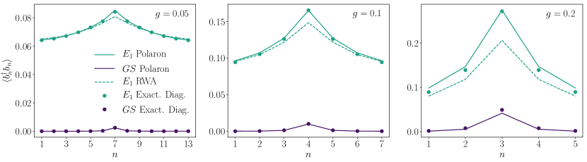
Figure 5: Comparison of spatial boson distributions from the PT, the RWA and exact diagonalisation. They correspond to $\Delta=0.3$, and $g=0.05$, $g=0.1$ and $g=0.2$ respectively from left to right. Solid lines are used to indicate Polaron results, dashed lines for RWA results and dots for exact diagonalisation results.

Finally, let us show that the bound state above the single-photon band that exists in the RWA ($\ket{E_{1}^{u}}$) Longo et al. (2010, 2011); Shi et al. (2016); Calajó et al. (2016), does not exist in general in the full model [(2)]. First of all, there are numerical evidences that the model [(2)] has, at least, an even bound state $\ket{E_{2}}$ Sánchez-Burillo et al. (2014). One can define a band of one-photon states over $\ket{E_{2}}$: $\ket{k,E_{2}}$ Sánchez-Burillo et al. (2018). The parity of these states is odd. The hypothetical bound state $\ket{E_{1}^{u}}$ would also be odd, since it has one excitation in the RWA limit. This implies that, in order for this state to exist, it cannot be embedded in the band formed by $\ket{k,E_{2}}$, since otherwise they would hybridize. A necessary condition is:

$$\omega_{0}\geq 4\lambda\,.$$ (23)

Otherwise, $\ket{E_{1}^{u}}$ does not exist. To demonstrate the latter, we note that the bound state energy is such that $E_{1}^{u}-E_{GS}>\omega_{0}+2\lambda$. On the other hand, $E_{2}-E_{GS}<2(\omega_{0}-2\lambda)$ (i.e. the two photon band). The overlap occurs (and thus the non-existence) if $E_{2}+\omega_{0}-2\lambda<E_{1}^{u}$. Putting it all together we arrive to the condition for existence given by Eq. (23). It seems a paradox, since this state does exist in the RWA for all $\omega_{0}$ and $\lambda$. The puzzle is solved by noting that in the full model this state becomes a resonance with a lifetime that diverges in the RWA limit.

III.3 Spontaneous emission

To end our analysis of the single-qubit model we discuss the behaviour of the system during spontaneous emission. We assume the atom-waveguide at the GS, then the qubit is driven within a $\pi$-pulse. After the $\pi$-pulse, the wavefunction is given by $\ket{\Psi(0)}=\sigma^{+}|GS\rangle$. Since $[\sigma_{x},U_{P}]=0$, we may work in the single excitation manifold in the Polaron picture. Employing the single excitation ansatz $|\psi\rangle_{P}=(\beta\sigma^{+}+\sum_{k}\beta_{k}a_{k}^{\dagger})|0;{\bf 0}\rangle$, the solution is obtained as the inverse Laplace transform $\beta(t)={\mathcal{L}}^{-1}[\beta(s)]$ with,

$$(s+i\Delta_{r})\beta(s)=1-\sum_{k}\frac{|\langle 0;{\bf 0}|a_{k}H_{P}\sigma^{+}|0;{\bf 0}\rangle|^{2}}{s+i\langle 0;{\bf 0}|a_{k}H_{P}a_{k}^{\dagger}|0;{\bf 0}\rangle}\;\beta(s)\;.$$ (24)

The properties of the (inverse) Laplace transform determine the spontanteous emission. In particular, since $\langle 0;{\bf 0}|a_{k}H_{P}\sigma^{+}|0;{\bf 0}\rangle|^{2}=2\Delta_{r}^{2}|f_{k}|^{2}$, in the continuum limit the sum in Eq. (24) can be converted to an integral over the spectral density $J(\omega)$. Let us discuss the two main contributions to this integral. Far from the band limits, $J(\omega)$ is sufficiently smooth and the main contribution comes from the poles in the sum, yielding the exponential decay $\exp[-J(\Delta_{r})t]$. Notice, that this is analogous to the RWA result (where the spontaneous emission is $J(\Delta)$) but now it is renormalized Zueco and García-Ripoll (2019). The other important feature is the long time dynamics of $\beta(t)$ which accounts for the qubit thermalization process. The final value theorem, $\lim_{s\to 0}s\beta(s)=\lim_{t\to\infty}\beta(t)$, tells that $\beta\neq 0$ if some divergence occurs in that integral. This occurs if bound states exist. Physically, this means that the initially excited state overlaps with the bound state John and Wang (1990); John and Quang (1994). This is conveniently calculated by chosing as a basis in the single excitation manifold,

$$\left\{\ket{E_{1}},\ket{E_{1}}^{\perp}_{p}\right\}.$$ (25)

Where $\ket{E_{1}}$ is the bound state and $\ket{E_{1}}^{\perp}_{p}$ are all other eigenstates orthogonal to it. We recall that the bound state can be written in terms of the original states spanning the one-excitation subspace

$$\ket{E_{1}}=\lambda_{0}\ket{1}\ket{0}+\sum_{k}\lambda_{k}\ket{0}\ket{1_{k}}.$$ (26)

The first term corresponds to the initial state of the system $\ket{\psi_{0}}=\ket{1}\ket{0}$, which indicates that the initial state has some projection on to the bound state,

$$\ket{\psi_{0}}=\lambda_{0}\ket{E_{1}}+\sum_{p}\lambda_{p}\ket{E_{1}}^{\perp}_{p}.$$ (27)

The projection onto the orthogonal basis states will contribute to the continuum and as such, it will not contribute the long time dynamics. The projection onto the bound state is responsible for the divergence and thus for the nonzero value for $\beta(t\to\infty)$. Doing the algebra and computing the observable (notice our return to the lab frame) we obtain that:

$$\langle\sigma^{z}(t\to\infty)\rangle=\lambda_{0}^{2}\expectationvalue{U_{P}^{\dagger}\sigma^{z}U_{P}}{E_{1}}-(1-\lambda_{0}^{2})\frac{\Delta_{r}}{\Delta}.$$ (28)

In Fig. 6 we confirm this expression. The evolution converges to the stationary value predicted by Eq. (28). Also shown in Fig. 6 is the difference with $\langle\sigma^{z}\rangle_{GS}$, which becomes significant as the ratio $g/\Delta$ increases, that is, as the system progresses into the USC regime. Let us emphasize that these results show that our theory is able to deal with the dynamics in USC confirming the peculiarities of the thermalisation process when both the light-matter coupling is non-perturbative and there exist excited bound states.

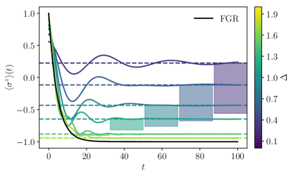
Figure 6: Evolution of $\langle\sigma^{z}\rangle$ (magnetization) for an initially excited qubit as a function of $\Delta$ for a fixed $g=0.3$. Solid coloured lines represent the simulated evolution while dashed coloured lines mark the stationary value predicted analytically, Eq. (28). For contrast, the solid black line corresponds to a Markovian evolution calculated by applying the FGR to the excited and ground states. Coloured shaded boxes have been used to showcase the difference between the stationary magnetisation for each $\Delta$ and the corresponding ground state magnetization, $\expectationvalue{\sigma^{z}}_{GS}$.

IV Two-qubit case

We tackle the case of two qubits coupled to the cavity array. Much like in the single qubit case, we first report the results for the ground state continuing with the bound states properties. We put emphasis in the qubit-qubit interactions mediated by the cavity array. As an application, we devise a simple state transfer between two distant qubits that uses those interactions.

IV.1 Ground state

Setting $N_{q}=2$ and $x=x_{1}-x_{2}$ in Eqs. (12) and (13) yields (see Apps. B.1- B.3) a spin model

$${\mathcal{H}}_{S}=\frac{\Delta_{r}}{2}\left(\sigma^{z}_{1}+\sigma_{2}^{z}\right)-\mathcal{J}\sigma_{1}^{x}\sigma_{2}^{x}+2\sum_{k}f_{k}(w_{k}f_{k}-2c_{k})$$ (29)

with $\mathcal{J}=2\sum_{k}f_{k}(2c_{k}-\omega_{k}f_{k})\cos(kx)$ which can be diagonalized to yield a ferromagnetic GS of the form

$$\ket{GS}_{S}=\cos\theta\ket{00}+\sin\theta\ket{11},$$ (30)

where $\ket{00}\equiv\ket{s_{1}=0,s_{2}=0}$ and the coefficients are

$$\cos\theta=\frac{\Delta_{r}+\sqrt{\Delta_{r}^{2}+\mathcal{J}^{2}}}{\sqrt{\left(\Delta_{r}+\sqrt{\Delta_{r}^{2}+\mathcal{J}^{2}}\right)^{2}+\mathcal{J}^{2}}}$$ (31)

$$\sin\theta=\frac{\mathcal{J}}{\sqrt{\left(\Delta_{r}+\sqrt{\Delta_{r}^{2}+\mathcal{J}^{2}}\right)^{2}+\mathcal{J}^{2}}}.$$ (32)

By Eq. (11), the GS mean energy is

$$\bar{E}_{GS}=-\sqrt{\Delta_{r}^{2}+\mathcal{J}^{2}}+2\sum_{k}f_{k}(w_{k}f_{k}-2c_{k}).$$ (33)

which is minimum for, see also Refs. McCutcheon et al. (2010); Zheng et al. (2015) and App. B.4 for a detailed derivation,

$$f_{k}=c_{k}\frac{\mathcal{E}+\mathcal{J}\cos(kx)}{\omega_{k}\mathcal{E}+\omega_{k}\mathcal{J}\cos(kx)+\Delta_{r}^{2}}.$$ (34)

We have introduced the constant $\mathcal{E}=\sqrt{\Delta_{r}^{2}+\mathcal{J}^{2}}$ to ease notation. It is immediate to check that, should the interaction constant ($\mathcal{J}$) vanish, we would recuperate the expression of $f_{k}$ that we found in the single-qubit case. This indeed happens when we set the qubits infinitely apart, as will be shown shortly. It is also evident that $f_{k}$ is even with respect to $k$, which matches the restriction we imposed so that the PT could be factored, see Eq. (10).

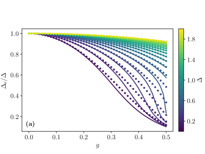
Figure 7: Renormalization of the bare frequency for $x=2$ as a function of $g$ and $\Delta$. Solid lines represent two-qubit results. Dots represent single-qubit results.

Figure 8 shows that the dependence of $\mathcal{J}$ with $x$ is exponential. This implies that the GS is a ferromagnetic state in a short-range Ising model. As such, in a multi-qubit scenario, only the interaction with first-nearest neighbours would have to be taken into account. Following our analysis of the single-qubit case, it is useful to study the renormalization of the bare frequency $\Delta$ with $g$. We have used a distance of $n=2$ sites to illustrate the deviation from the results obtained in the one-qubit scenario.

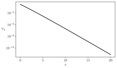
Figure 8: Dependence of the Ising constant, $\mathcal{J}$, with the distance between the qubits, $x$. The behaviour is analogous for all values of $g$.

Figure 7(b) shows that the influence of the neighbouring qubit sharpens the renormalization process, making the system go into full renormalization at lower values of $g$. Granted, this effect vanishes if one places the qubits further apart. Due to the exponential decay of $\mathcal{J}$, we have found that at distances of around $20$ sites the results obtained for one and two qubits are indistinguishable.

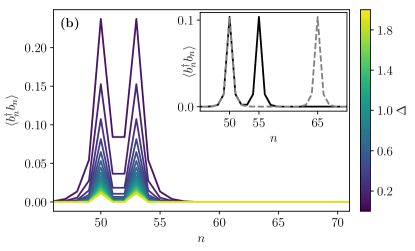
Figure 9: Spatial distribution of GS the photons for $g=0.3$ and $x=3$ as a function of $\Delta$, with inset showing the difference in photon cloud localisation when the qubits are placed at distances $x=5$ and $x=15$ for $g=0.3$ and $\Delta=0.3$.

Back when we studied the single-qubit system we showed that the probability of having an excited spin state was an observable directly related to the renormalization of the bare frequency. The extension to two qubits is straightforward

$$P_{e}=\frac{2+\expectationvalue{\sigma_{1}^{z}+\sigma_{2}^{z}}{GS}_{S}}{2}=1-\frac{\Delta_{r}}{\Delta}\left(\cos^{2}{\theta}-\sin^{2}{\theta}\right)$$ (35)

Where $\ket{GS}_{S}=\cos\theta\ket{00}+\sin\theta\ket{11}$ now. Notice that at large distances, as $\mathcal{J}\to 0$ then $\cos\theta\rightarrow 1$ and $\sin\theta\rightarrow 0$, so Eq. (35) reduces to twice the probability found for a single qubit [Eq. (18)]. The effect of the Ising interaction is revealed at short distances where $P_{e}$ deviates from the single-qubit result, no longer equating to the sum of two non-interacting spins. We can again probe the spatial localisation of the bosonic cloud. Following the scheme presented in the single-qubit case, we obtain

$$\expectationvalue{b_{n}^{\dagger}b_{n}}=|f_{n,1}|^{2}+|f_{n,2}|^{2}+2\cos\theta\sin\theta\Re{f^{*}_{n,1}f_{n,2}},$$ (36)

where

$$f_{n,j}=\frac{1}{\sqrt{N}}\sum_{k}e^{ikx_{j}}f_{k}e^{-ik(n-N/2)}.$$ (37)

See App. B.5 for details on this calculation. It is interesting to see the overlap between the two bosonic clouds surrounding each qubit. Figure 9 shows this phenomenon for a value of $n=3$ where the overlap is significant. In the same figure, the inset monitors the effect of the coalescence of the clouds as the two qubits approach each other.

IV.2 Bound states

Analogously to the single-qubit case, we seek an effective Hamiltonian for the two-qubit model that is a good approximation of the full Hamiltonian but conserves the number of excitations, allowing us to restrict our search for bound states to the one-excitation subspace. We have discussed how $f_{k}$ for two-qubits converges to the expression of $f_{k}$ for a single qubit, so if we assume $\mathcal{J}$ to be small, we can write

$$f_{k}=f_{k}^{0}+\delta(f_{k}).$$ (38)

This allows us to reach the effective Hamiltonian

$$\begin{split}H_{P}=&\frac{\Delta_{r}}{2}\left(\sigma_{1}^{z}+\sigma_{2}^{z}\right)-2\Delta_{r}\sum_{j}\sigma_{j}^{z}\sum_{k,p}f_{k}f_{p}e^{i(k-p)x_{j}}b_{k}^{\dagger}b_{p}\\ +&\sum_{j,k}\left(2\Delta_{r}f_{k}^{0}+\delta(f_{k})(\Delta_{r}-\omega_{k})\right)\left(\sigma_{j}^{-}b_{k}^{\dagger}e^{ikx_{j}}+{\rm h.c.}\right)\\ +&\sum_{k}\omega_{k}b_{k}^{\dagger}b_{k}-\mathcal{J}\sigma_{1}^{x}\sigma_{2}^{x}+E_{ZP}.\end{split}$$ (39)

By construction, the GS obtained by applying the variational method is an eigenstate of $H_{P}$ and the eigenvalue also coincides with the variational energy.

Once again, we can diagonalise the restriction of $H_{P}$ in search of states whose energy lies below the band limit and are, thus, bound. In this case, we expect to find two bound states, corresponding to the symmetric and antisymmetric combination of the wavefunctions corresponding to each single-qubit bound state (See Fig. 10).

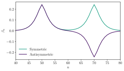
Figure 10: Symmetric and antisymmetric bound state wave functions for $g=0.3$, $\Delta=0.3$ and $x=20$. Solid lines represent Polaron results and dashed lines represent RWA results.

A general eigenstate of $H_{P}$ has the form

$$|\psi\rangle_{P}=(\beta_{1}\sigma_{1}^{+}+\beta_{2}\sigma_{2}^{+}+\sum_{k}\beta_{k}a_{k}^{\dagger})\ket{GS}.$$ (40)

The reader might recall that in the single-qubit case the one-excitation subspace was spanned by $\ket{1}\ket{0}$ and $\ket{0}\ket{1_{k}}$ and wonder why we cannot substitute $\ket{S}\ket{1_{k}}$ by $\ket{00}\ket{1_{k}}$ in the two-qubit basis. In that sense, it must be clarified that we seek to work in a subspace that is one excitation above the GS, regardless of however many excitations the GS contains. The proposed state, Eq. (40), on the other hand, comes with a problem since the subspace spanned by Eq. (40) is not closed under the action of the Hamiltonian, e.g. $\sigma_{1}^{-}a_{k}^{\dagger}|10\rangle|0_{k}\rangle=\cos(\theta)|GS\rangle_{S}|1_{k}\rangle+\sin(\theta)(-\sin(\theta)|00\rangle+\cos(\theta)|11\rangle|1_{k}\rangle)$. Fortunately, this second contribution is of second order in $f_{k}$. Besides, the terms containing $\sigma_{1}^{-}a_{k}^{\dagger}$ in Hamiltonian [(39)] are of the order of $f_{k}$. Thus they are h.o.t that, consistently with Eq. (21), are discarded.
Figure 10 shows $\beta_{n}$ for the two lowest energy eigenstates. Where $\lambda_{n}$ is obtained by Fourier transforming $\lambda_{k}$ in Eq. (40). In the single-qubit case, we showed that there exists a bound state in the form of a cloud of virtual photons localised around the qubit. We have also shown that two sufficiently distant qubits do no interact and, as such, their wavefunctions do not overlap, contributing two bound states of equal energy to the spectrum. As the two qubits approach, we expect the increasing overlap to break the degeneracy, and split the two bound states into different energies. If that is the case, the interaction can cause the energy of the antisymmetric state to rise above the lower band limit, forcing it to no longer be bound (nor antisymmetric), as the corresponding photons have an allowed frequency in the waveguide, and as such they no longer exhibit exponential decay. These oscillating eigenstates are referred to as scattering states Sánchez-Burillo et al. (2017). Figure 11 shows the aforementioned effect. In the figure we also compare our results wich the ones obtained within the RWA. We conclude that the latter understimates the interaction between the two bound states (see below). In Fig. 12 a comparison between the spatial distribution of photons for two different distances is drawn. As the two qubits approach, the difference in profiles becomes significant, and, should they reach $n=2$, the antisymmetric bound state would cease to exist as it enters the allowed frequency band. See App. B.6 for a calculation of $\expectationvalue{b^{\dagger}_{n}b_{n}}$.

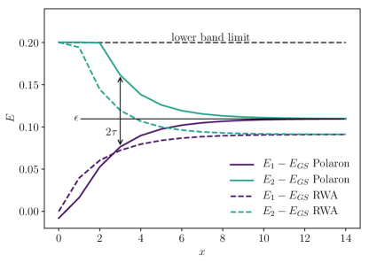
Figure 11: Energy diference between symmetric and antisymmetric bound states as a function of $x$, the distance between qubits for $g=0.3$ and $\Delta=0.3$. Dashed lines represent RWA results and solid lines represent Polaron results.

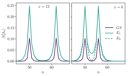
Figure 12: Comparison of spacial photon distributions of the symmetric ($E_{1}$) and antisymmetric ($E_{2}$) bound states for $g=0.3$ and $\Delta=0.3$ at two different distances, $x=12$ and $x=6$.

IV.3 State transfer

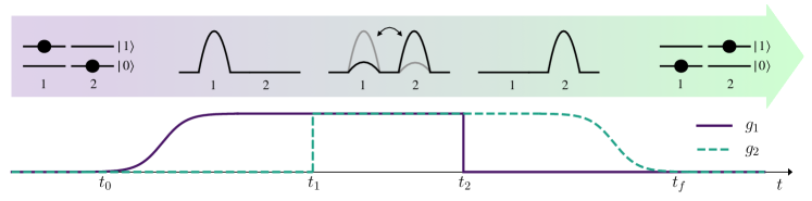
Figure 13: State transfer protocol between two qubits coupled to the same linear cavity array with distinct tunable coupling constants $g_{1}$ and $g_{2}$. Bound states are depicted as parabolic instead of exponential for aesthetic purposes.

Inspired by Fig. 11 and restricting ourselves to the two bound states we can define a tight-binding Hamiltonian

$$H_{TB}=\sum_{i={L,R}}\epsilon\ket{i}\bra{i}+\sum_{\begin{subarray}{c}i,j=L,R\\ i\neq j\end{subarray}}\tau\ket{i}\bra{j},$$ (41)

where $\ket{L}$ represents the bound state of the left-most qubit and $\ket{R}$ represents the bound state of the right-most one. The eigenstates of $H_{TB}$ are the symmetric and antisymmetric combinations of $\ket{L}$ and $\ket{R}$, provided $\tau\neq 0$, with respective energies $\epsilon-\tau$ and $\epsilon+\tau$. This simplified model is the basis for the study of effective interactions between bound states, which, as we introduced, provides a means to engineer lossless state transfer protocols through virtual photons, one of the main objectives of our work. Real, propagating photons can be used to transport information between distant qubits, but, even in one-dimensional arrays where an emitted photon travels non-dissipatively, there exist undesired losses intrinsic to the emission process. The reason is simple, in the absence of anisotropies, it is equally likely that a radiated photon will travel in the direction of the neighbouring qubit as it is for it to travel in the opposite direction, and thus be lost. The transmission of information via virtual photons bypasses this limitation. By virtue of them being non-radiative, there is no loss, information is shared between close qubits through the overlap of their photonic clouds.
To exemplify perfect lossless state-transfer using bound states, we propose the protocol shown in Fig. 13. Its purpose is to transfer the excited state from one qubit to the other deterministically. First, the left-most qubit is initialized in its excited state and the other is kept in its ground state while both are un-coupled from the waveguide. We assume that $g_{1}$ and $g_{2}$, the coupling constant of each qubit to the waveguide, can be tuned independently, and so at $t_{0}$, $g_{1}$ is increased adiabatically, so that the excited qubit entangles with the waveguide progressively, to become a bound-state, by means of the Adiabatic Theorem. Then, at $t_{1}$, $g_{2}$ is increased diabatically to match $g_{1}$. This sudden change in the Hamiltonian does not allow the state to evolve quasi-statically into the new eigenstate and instead gives rise to Rabi oscillations between the left and right bound states, whose symmetric and antysimmetric combinations are actually the eigenstates of the new Hamiltonian. Knowing the hopping frequency ($\tau$), we can interrupt the dynamics, by diabatically zeroing $g_{1}$ at $t_{2}$, at the precise moment where the system is fully in the right bound state. Finally, $g_{2}$ is lowered adiabatically, so the right bound state transforms into an excited right-most qubit, succesfully completing the state-transfer protocol at $t_{f}$. This protocol can be applied sequentially to a succession of qubits, to effectively transport a state along the waveguide.

It is important to note that this method is limited by the fact that the interaction decays exponentially, and this limitation is twofold. Firstly, an exponential decay means that, in order to transport a state between distant qubits, many ancilla quibts are required, placed in close formation, so that there exists an effective interaction amongst every pair of consecutive qubits. For every qubit added to the chain, the system becomes more susceptible to decoherence and losses. In addition, the hopping frequency ($\tau$), which is proportional to the coupling, is what determines the speed at which a single iteration of the protocol can be performed, so it is against our interest that the coupling decays so rapidly. One may even doubt if an exponentially decaying effective interaction would be, at any range, intense enough to not be overpowered by spurious dipole-dipole interactions between the qubits, which decay more slowly, with a power-law. Fortunately, we can assure that the effective interaction is orders of magnitude greater than dipole-dipole interactions, since the latter is of the order of $10^{-4}\ eV$ for nearest neighbours withing a crystal lattice ($d\sim 1\text{\AA}$) . In our set up, there is a non-negligible interaction up to distances of around $3$ sites, which in experimental realisations of quantum circuits have sizes of millimetres.

V Conclusions

We have discussed the main properties of bound states in waveguide QED beyond the RWA paradigm. In other words, we have quantified the corrections to the standard calculations where the qubits-photons interaction is assumed to be number conserving based on the perturbative character of the latter. We have shown that the Polaron technique is useful. It provides a unitary transformation that disentangles qubits and waveguide and the interaction, within this picture, is effectively number conserving. Therefore, it allows to export techniques as the Weisskopf-Wigner theory and intuitions to a broader range of light-matter coupling strengths where the RWA fails.
The main results discussed in the paper are as follows. We have extended the calculations for the spontaneous emission up to moderate light-matter couplings obtaining a renormalization of the rate (due to the qubit-frequency renormalization). The existence criteria for bound states has been generalised and its role in the thermalization of the qubits has been discussed. Finally, we have computed the effective spin-spin interactions both through vacuum fluctuations and bound states. We sketched a perfect state transfer protocol among bound states.

VI Acknowledgments

This work has been supported by the EU (COST Ac- tion 15128 MolSpin on Molecular Spintronics, QUAN- TERA SUMO project and the Spanish MICINN grant MAT2017- 89993-R. Juan Román-Roche is supported by ICMA through a Pi2 contract. Eduardo Sánchez-Burillo acknowledges ERC Advanced Grant QUENOCOBA under the EU Horizon 2020 program (grant agreement 742102).

Appendix A Single qubit: some details of the calculations

A.1 Derivation of the basic commutation relations

Let $A$, $B$, and $C$ be operators such that $[B,A]=C$. Then, if $[C,A]=0$ it follows that $[B,A^{n}]=nCA^{n-1}$.

The proof is by induction:

$$[B,A^{n}] =[B,AA^{n-1}]$$

$$=A[B,A^{n-1}]+[B,A]A^{n-1}$$

$$\text{by I.H.}\rightarrow =A(n-1)CA^{n-2}+CA^{n-1}$$

$$[C,A]=0\rightarrow =(n-1)CA^{n-1}+CA^{n-1}$$

$$=nCA^{n-1}$$ (42)

From this, one can prove that $[B,e^{A}]=Ce^{A}$ also holds.

$$[B,e^{A}] =\sum_{n=0}\frac{[B,A^{n}]^{n}}{n!}$$

$$=[A,I]+\sum_{n=1}\frac{[B,A^{n}]^{n}}{n!}$$

$$=\sum_{n=1}\frac{nCA^{n-1}}{n!}=C\sum_{n=1}\frac{A^{n-1}}{(n-1)!}$$

$$=C\sum_{n=0}\frac{A^{n}}{n!}=Ce^{A}$$ (43)

If we express the Polaron transform as $U_{P}=\exp[A]$, we can apply the properties we just proved to arrive at the basic commutation relations.

$$[b_{k},A]=-\sigma^{x}\left(f_{k}[b_{k},b^{\dagger}_{k}]-f_{k}^{*}[b_{k},b_{k}]\right)=-f_{k}\sigma^{x}\rightarrow$$

$$[b_{k},U_{P}]=-f_{k}\sigma^{x}U_{P}$$ (44)

$$[b^{\dagger}_{k},A]=-\sigma^{x}\left(f_{k}[b^{\dagger}_{k},b^{\dagger}_{k}]-f_{k}^{*}[b^{\dagger}_{k},b_{k}]\right)=-f_{k}\sigma^{x}\rightarrow$$

$$[b^{\dagger}_{k},U_{P}]=-f_{k}^{*}\sigma^{x}U_{P}$$ (45)

A.2 Calculation of $\expectationvalue{b_{n}^{\dagger}b_{n}}$ for the GS of a single qubit

$$\expectationvalue{b_{n}^{\dagger}b_{n}} =\expectationvalue{b_{n}^{\dagger}b_{n}}{GS}$$

$$=\expectationvalue{\frac{1}{\sqrt{N}}\sum_{k}e^{ik(n-N/2)}b_{k}^{\dagger}\frac{1}{\sqrt{N}}\sum_{p}e^{-ip(n-N/2)}b_{p}}{GS}$$

$$=\frac{1}{N}\sum_{k,p}e^{i(k-p)(n-N/2)}\expectationvalue{U_{p}^{\dagger}b_{k}^{\dagger}b_{p}U_{p}}{00}$$ (46)

In order to continue, we must first calculate $U_{p}^{\dagger}b_{k}^{\dagger}b_{p}U_{p}$. Since we have already taken $f_{k}$ as real in previous calculations, we assume it to be real here as well.

$$U_{p}^{\dagger}b_{k}^{\dagger}b_{p}U_{p} =U_{P}^{\dagger}\left(b^{\dagger}_{k}[b_{p},U_{P}]+[b^{\dagger}_{k},U_{P}]b_{p}\right)+b_{k}^{\dagger}b_{p}$$

$$=U_{P}^{\dagger}\left(-f_{p}\sigma^{x}b^{\dagger}_{k}U_{P}-f_{k}\sigma^{x}U_{P}b_{p}\right)+b_{k}^{\dagger}b_{p}$$

$$=U_{P}^{\dagger}\left(-f_{p}\sigma^{x}[b^{\dagger}_{k},U_{P}]-f_{p}\sigma^{x}U_{P}b^{\dagger}_{k}-f_{k}\sigma^{x}U_{P}b_{p}\right)+b_{k}^{\dagger}b_{p}$$

$$=U_{P}^{\dagger}\left(U_{P}f_{k}f_{p}-f_{p}\sigma^{x}U_{P}b^{\dagger}_{k}-f_{k}\sigma^{x}U_{P}b_{p}\right)+b_{k}^{\dagger}b_{p}$$

$$=f_{k}f_{p}-\sigma^{x}(f_{p}b_{k}^{\dagger}+f_{k}b_{p})+b_{k}^{\dagger}b_{p}$$ (47)

We are now equipped with the necessary ingredients to compute $\expectationvalue{U_{p}^{\dagger}b_{k}^{\dagger}b_{p}U_{p}}{00}$. Considering that the state $\ket{00}$ does not connect through the second and third terms, the mean value is just $f_{k}f_{p}$.

With that, we simply have

$$\expectationvalue{b_{n}^{\dagger}b_{n}}=\frac{1}{\sqrt{N}}\sum_{k}e^{ik(n-N/2)}f_{k}\frac{1}{\sqrt{N}}\sum_{p}e^{-ip(n-N/2)}f_{p}=f_{n}^{*}f_{n}=f_{n}^{2}.$$ (48)

A.3 Exponential localisation of the GS

We recall that

$$f_{k}=\frac{g}{\sqrt{N}(\Delta_{r}+\omega_{k})}$$ (49)

with

$$\omega_{k}=\omega_{0}-2\lambda\cos k$$ (50)

Noticing that

$$\mathcal{F}[\;e^{-\kappa_{\rm GS}|n-N/2|}\;]=\frac{1}{\sqrt{N}}\frac{1-e^{-2\kappa_{\rm GS}}}{1+e^{-2\kappa_{\rm GS}}+2e^{-\kappa_{\rm GS}}\cos{k}}$$ (51)

with our convention for the Fourier transform $\mathcal{F}[g(n)]=\sum_{0}^{N-1}e^{ik(n-N/2)}\;g(n)$. Therefore,

$$\mathcal{F}[\;e^{-\kappa_{\rm GS}|n-N/2|}\;]\sim f_{k}$$ (52)

with the identifications

$$\lambda \sim e^{-\kappa_{\rm GS}}$$ (53a)

$$\omega_{0}+\Delta_{r} \sim 1+e^{-2\kappa_{\rm GS}},$$ (53b)

which yields Eq (20) in the main text.

A.4 Single qubit effective Hamiltonian

The strict application of the Polaron transform to the original Hamiltonian, $H_{P}=U_{P}^{\dagger}HU_{P}$, yields the transformed Hamiltonian

$$H_{P}=\frac{\Delta}{2}\exp[2\sigma^{x}\sum_{k}f_{k}b^{\dagger}_{k}-f_{k}^{*}b_{k}]\sigma^{z}+\sum_{k}\omega_{k}b_{k}^{\dagger}b_{k}+\Delta_{r}{\sigma^{x}}\sum_{k}f_{k}\left(b_{k}^{\dagger}+b_{k}\right)+E_{ZP}.$$ (54)

We can further simplify it by expanding the exponential term. Making use of the Baker-Campbell-Hausdorff formula and taking $\{f_{k}\}$ real we get

$$\exp[2\sigma^{x}\sum_{k}f_{k}b^{\dagger}_{k}-f_{k}b_{k}]=\exp[-2\sum_{k}f_{k}^{2}]\exp[2\sigma^{x}\sum_{k}f_{k}b^{\dagger}_{k}]\exp[-2\sigma^{x}\sum_{k}f_{k}b_{k}].$$ (55)

A power series expansions of the non constant terms gives

$$\exp[2\sigma^{x}\sum_{k}f_{k}b^{\dagger}_{k}] =1+2\sigma^{x}\sum_{k}f_{k}b^{\dagger}_{k}+\dots,$$ (56)

$$\exp[-2\sigma^{x}\sum_{k}f_{k}b_{k}] =1-2\sigma^{x}\sum_{k}f_{k}b_{k}+\dots.$$ (57)

Ignoring higher order terms, the right hand side of Eq. (55) becomes

$$\exp[-2\sum_{k}f_{k}^{2}]\left(1+2\sigma^{x}\sum_{k}f_{k}\left(b^{\dagger}_{k}-b_{k}\right)-4\sum_{k,p}f_{k}f_{p}b^{\dagger}_{k}b_{p}\right).$$ (58)

Reintroducing this result in $H_{P}$ yields

$$\begin{split}H_{P}&=\frac{\Delta_{r}}{2}\sigma^{z}+\Delta_{r}\sigma^{x}\sigma^{z}\sum_{k}f_{k}\left(b^{\dagger}_{k}-b_{k}\right)-2\Delta_{r}\sum_{k,p}f_{k}f_{p}b^{\dagger}_{k}b_{p}\\ &+\sum_{k}\omega_{k}b^{\dagger}_{k}b_{k}+\Delta_{r}{\sigma^{x}}\sum_{k}f_{k}\left(b_{k}^{\dagger}+b_{k}\right)+E_{ZP}.\end{split}$$ (59)

Considering that $\sigma^{x}\sigma^{z}+\sigma^{x}=2\sigma^{-}$ and $-\sigma^{x}\sigma^{z}+\sigma^{x}=2\sigma^{+}$ we can combine the second and second-to-last terms to arrive at the final expression for $H_{P}$

$$H_{\text{eff}}=\frac{\Delta_{r}}{2}\sigma^{z}+\sum_{k}\omega_{k}b^{\dagger}_{k}b_{k}+2\Delta_{r}\sum_{k}f_{k}\left(\sigma^{-}b^{\dagger}_{k}-\sigma^{+}b_{k}\right)-2\Delta_{r}\sum_{k,p}f_{k}f_{p}b^{\dagger}_{k}b_{p}+E_{ZP}.$$ (60)

A.5 Calculation of $\expectationvalue{b_{n}^{\dagger}b_{n}}$ for the SEBS of a single qubit

The SEBS will be a state of the form

$$\ket{v}=\lambda_{0}\ket{1}\ket{0}+\sum_{k}\lambda_{k}\ket{0}\ket{1_{k}}.$$ (61)

Thus

$$\expectationvalue{b_{n}^{\dagger}b_{n}} =\expectationvalue{b_{n}^{\dagger}b_{n}}{v}$$

$$=\expectationvalue{\frac{1}{\sqrt{N}}\sum_{k}e^{ik(n-N/2)}b_{k}^{\dagger}\frac{1}{\sqrt{N}}\sum_{p}e^{-ip(n-N/2)}b_{p}}{v}$$

$$=\frac{1}{N}\sum_{k,p}e^{i(k-p)(n-N/2)}\expectationvalue{U_{p}^{\dagger}b_{k}^{\dagger}b_{p}U_{p}}{v}.$$ (62)

In App. A.2 we saw that $U_{p}^{\dagger}b_{k}^{\dagger}b_{p}U_{p}=f_{k}f_{p}-\sigma^{x}(f_{p}b_{k}^{\dagger}+f_{k}b_{p})+b_{k}^{\dagger}b_{p}$ . The first term is constant so $\ket{v}$ connects entirely yielding $f_{k}f_{p}$. The last term only connects the bosonic part of $\ket{v}$ to give $\lambda_{k}\lambda_{p}$. Finally, the second term cross-connects the two components of $\ket{v}$ resulting in $\lambda_{0}f_{p}\lambda^{*}_{k}+\lambda_{0}f_{k}\lambda_{p}$. Reintroducing these partial results into Eq. (87) one has

$$\expectationvalue{b_{n}^{\dagger}b_{n}}=f_{n}^{2}+\lambda_{n}^{2}+\lambda_{0}f_{n}^{*}\lambda^{*}_{n}+\lambda_{0}f_{n}\lambda_{n}=f_{n}^{2}+\lambda_{n}^{2}+2\lambda_{0}\Re{f_{n}\lambda_{n}}.$$ (63)

A.6 Existence of bound states in USC

We work in the Polaron picture. A non-normalized single excitation is,

$$|\psi_{1}\rangle_{P}=\lambda_{0}|1,0\rangle+\sum\lambda_{k}|0,1_{k}\rangle$$ (64)

It is an eigenstate iff

$$\Delta_{r}-\sum\lambda_{k}2\Delta_{r}f_{k} =E$$ (65a)

$$\lambda_{k}\omega_{k}-2\Delta_{r}f_{k}+2\Delta_{r}\lambda_{k}\sum_{k^{\prime}}f_{k}f_{k^{\prime}} =E\lambda_{k}$$ (65b)

The solution for $E$ is found by searching the zeros of the function $F(E)$ [Cf. with the RWA case in Ref. Shi et al., 2016]

$$F_{1}(E)=E-\left(\Delta_{r}+\sum_{k}\frac{(2\Delta_{r}f_{k})^{2}}{E-\omega_{k}-2\Delta_{r}\sum_{k^{\prime}}f_{k}f_{k^{\prime}}}\right)\;.$$ (66)

If $E<{\rm min}[\omega_{k}]$, the state is a SEBS. Notice that the term in brackets is is a monotonically decreasing function with $g$. Therefore if a bound state exists for $g\to 0^{+}$ then it will exists for any finite value of $g$. For our model in the limit $g\to 0^{+}$ a bound state below the band exists Shi et al. (2016), thus the existence of bound states in the USC is guaranteed.

A.7 Localization lenght

Apart from their existence the key property of bound states is their localization lenght. From, Eq. (65b) we obtain that:

$$\lambda_{k}=\frac{2\Delta_{r}f_{k}}{\omega_{k}-E_{1}+2\Delta_{r}\sum_{k^{\prime}}f_{k}f_{k^{\prime}}}$$ (67)

In the log $g$-regime $2\Delta_{r}f_{k}\sim g$ and we can neglect the term $2\Delta_{r}\sum_{k^{\prime}}f_{k}f_{k^{\prime}}$, therefore by simple inspection we see that $\mathcal{F}^{-1}[\lambda_{k}]=\lambda_{n}\sim e^{-\kappa n}$ with

$$\kappa_{1}\cong\text{arccosh}\left(\frac{\omega_{0}-E_{1}}{2\mathcal{J}}\right)$$ (68)

Looking at Eq. (63), Section A.3 and Eq. (20) the localization is given by $\kappa_{\rm SEBS}^{-1}=\max(\kappa_{\rm GS}^{-1},\kappa^{-1})$ as given by Eq. (22).

Appendix B Calculations for the two-qubit case

B.1 Derivation of the basic commutation relations

Recycling much of the work done in Ap. A.1 we simply see that

$$[b_{k},A_{j}]=-\sigma_{j}^{x}\left(f_{k}e^{ikx_{j}}[b_{k},b_{k}^{\dagger}]-f_{k}e^{-ikx_{j}}[b_{k},b_{k}]\right)=-\sigma^{x}f_{k}e^{ikx_{j}}\rightarrow$$

$$[b_{k},U_{j}]=-\sigma^{x}f_{k}e^{ikx_{j}}U_{j}$$ (69)

$$[b_{k}^{\dagger},A_{j}]=-\sigma_{j}^{x}\left(f_{k}e^{ikx_{j}}[b_{k}^{\dagger},b_{k}^{\dagger}]-f_{k}e^{-ikx_{j}}[b_{k}^{\dagger},b_{k}]\right)=-\sigma^{x}f_{k}e^{-ikx_{j}}\rightarrow$$

$$[b_{k}^{\dagger},U_{j}]=-\sigma^{x}f_{k}e^{-ikx_{j}}U_{j}.$$ (70)

B.2 Calculation of $H_{I}$

In an attempt to lighten notation we have omitted the summation signs ($\sum$) in the following calculation. They will be reintroduced when we present the final result. It must be understood that there is summation over all indexes present, for instance

$$\sigma^{x}_{j}c_{k}\left(b_{k}^{\dagger}e^{ikx_{j}}+b_{k}e^{-ikx_{j}}\right)\equiv\sum_{j}\sigma^{x}_{j}\sum_{k}c_{k}\left(b_{k}^{\dagger}e^{ikx_{j}}+b_{k}e^{-ikx_{j}}\right).$$ (71)

We thus have

$$U_{P}^{\dagger}H_{I}U_{P}=U_{2}^{\dagger}U_{1}^{\dagger}\left(H_{I}^{1}+H_{I}^{2}\right)U_{1}U_{2},$$ (72)

we can focus on $H_{I}^{1}$ and the results will be perfectly extensible to $H_{I}^{2}$.

Hence, making use of the basic commutation relations, [Eqs. (69), (70)],

$$U_{2}^{\dagger}U_{1}^{\dagger}H_{I}^{1}U_{1}U_{2} =U_{2}^{\dagger}U_{1}^{\dagger}\sigma^{x}_{1}c_{k}\left(b_{k}^{\dagger}e^{ikx_{1}}+b_{k}e^{-ikx_{1}}\right)U_{1}U_{2}$$

$$=U_{2}^{\dagger}\left(\sigma_{1}^{x}c_{k}\left(-\sigma_{1}^{x}e^{ikx_{1}}f_{k}e^{-ikx_{1}}-\sigma_{1}^{x}e^{-ikx_{1}}f_{k}e^{ikx_{1}}\right)+H_{I}^{1}\right)U_{2}$$

$$=U_{2}^{\dagger}\left(-2c_{k}f_{k}+H_{I}^{1}\right)U_{2}=-2c_{k}f_{k}+U_{2}^{\dagger}H_{I}^{1}U_{2}$$

$$=-2c_{k}f_{k}+U_{2}^{\dagger}\left(\sigma_{1}^{x}c_{k}\left(b_{k}^{\dagger}e^{ikx_{1}}+b_{k}e^{-ikx_{1}}\right)\right)U_{2}$$

$$=-2c_{k}f_{k}+\sigma_{1}^{x}c_{k}\left(-\sigma_{2}^{x}e^{ikx_{1}}f_{k}e^{-ikx_{2}}-\sigma_{2}^{x}e^{-ikx_{1}}f_{k}e^{ikx_{2}}\right)+H_{I}^{1}$$

$$=-2c_{k}f_{k}-2\sigma_{1}^{x}\sigma_{2}^{x}c_{k}f_{k}\cos(kx)+H_{I}^{1}.$$ (73)

Likewise,

$$U_{2}^{\dagger}U_{1}^{\dagger}H_{I}^{2}U_{1}U_{2}=-2c_{k}f_{k}-2\sigma_{1}^{x}\sigma_{2}^{x}c_{k}f_{k}\cos(kx)+H_{I}^{2}.$$ (74)

And finally,

$$U_{P}^{\dagger}H_{I}U_{P}=-4\sum_{k}c_{k}f_{k}-4\sigma_{1}^{x}\sigma_{2}^{x}\sum_{k}c_{k}f_{k}\cos(kx)+H_{I}.$$ (75)

B.3 Calculation of $H_{B}$

Much like in App. B.2 we have omitted the summation signs for the calculation.

$$U_{P}^{\dagger}H_{B}U_{P} =U_{2}^{\dagger}U_{1}^{\dagger}\omega_{k}b_{k}^{\dagger}b_{k}U_{1}U_{2}$$

$$=\omega_{k}U_{2}^{\dagger}\left(U_{1}^{\dagger}\left(b_{k}^{\dagger}[b_{k},U_{1}]+[b_{k}^{\dagger},U_{1}]b_{k}\right)+H_{B}/\omega_{k}\right)$$

$$=\omega_{k}U_{2}^{\dagger}\left(U_{1}^{\dagger}\left(-\sigma_{1}^{x}b_{k}^{\dagger}f_{k}e^{ikx_{1}}U_{1}-\sigma f_{k}e^{-ikx_{1}}U_{1}b_{k}\right)+H_{B}/\omega_{k}\right)U_{2}$$

$$=\omega_{k}U_{2}^{\dagger}\left(U_{1}^{\dagger}\left(-\sigma_{1}^{x}f_{k}e^{ikx_{1}}\left(U_{1}b_{k}^{\dagger}-\sigma_{1}^{x}f_{k}e^{-ikx_{1}}U_{1}\right)-\sigma_{1}^{x}f_{k}e^{-ikx_{1}}U_{1}b_{k}\right)+H_{B}/\omega_{k}\right)U_{2}$$

$$=\omega_{k}U_{2}^{\dagger}\left(-\sigma_{1}^{x}f_{k}\left(b_{k}^{\dagger}e^{ikx_{1}}+b_{k}e^{-ikx_{1}}\right)+f_{k}^{2}+H_{B}/\omega_{k}\right)U_{2}$$

$$=H_{B}+\omega_{k}\left(2f_{k}^{2}-\sigma_{1}^{x}f_{k}\left(b_{k}^{\dagger}e^{ikx_{1}}+b_{k}e^{-ikx_{1}}\right)-\sigma_{2}^{x}f_{k}\left(b_{k}^{\dagger}e^{ikx_{2}}+b_{k}e^{-ikx_{2}}\right)\right.$$

$$\left.\quad\quad\quad\quad\quad\quad+\ U_{2}^{\dagger}\left[-\sigma_{1}^{x}f_{k}\left(b_{k}^{\dagger}e^{ikx_{1}}+b_{k}e^{-ikx_{1}}\right),U_{2}\right]\right)$$

$$=H_{B}+\omega_{k}\left(2f_{k}^{2}-\sigma_{j}^{x}f_{k}\left(b_{k}^{\dagger}e^{ikx_{j}}+b_{k}e^{-ikx_{j}}\right)\right.$$

$$\left.\quad\quad\quad\quad\quad\quad-\ \sigma_{1}^{x}f_{k}\left(-\sigma_{2}^{x}e^{ikx_{1}}f_{k}e^{-ikx_{2}}-\sigma_{2}^{x}e^{-ikx_{1}}f_{k}e^{ikx_{2}}\right)\right)$$

$$=\omega_{k}\left(2f_{k}^{2}-\sigma_{j}^{x}f_{k}\left(b_{k}^{\dagger}e^{ikx_{j}}+b_{k}e^{-ikx_{j}}\right)+2\sigma_{1}^{x}\sigma_{2}^{x}f_{k}^{2}\cos(k(x_{2}-x_{1}))\right)+H_{B}$$ (76)

So finally,

$$\begin{split}U_{P}^{\dagger}H_{B}U_{P}=&\ 2\sum_{k}\omega_{k}f_{k}^{2}+2\sigma_{1}^{x}\sigma_{2}^{x}\sum_{k}\omega_{k}f_{k}^{2}\cos(kx)\\ &-\sum_{j}\sigma_{j}^{x}\sum_{k}\omega_{k}f_{k}\left(b_{k}^{\dagger}e^{ikx_{j}}+b_{k}e^{-ikx_{j}}\right)+\sum_{k}\omega_{k}b_{k}^{\dagger}b_{k}.\end{split}$$ (77)

B.4 Calculation of the minimal value of $f_{k}$

The explicit dependence of $\bar{E}_{GS}$ with $f_{k}$ is

$$\bar{E}_{GS} =-\mathcal{E}+2\sum_{k}f_{k}(\omega_{k}f_{k}-2c_{k})=-\sqrt{\Delta_{r}^{2}+\mathcal{J}^{2}}+2\sum_{k}f_{k}(\omega_{k}f_{k}-2c_{k})$$

$$\begin{split}&=-\sqrt{4\left(\sum_{k}f_{k}(2c_{k}-\omega_{k}f_{k})\cos(kx)\right)^{2}+\Delta^{2}\exp[-4\sum_{k}f_{k}^{2}]}\\ &\quad\quad+2\sum_{k}f_{k}(\omega_{k}f_{k}-2c_{k}).\end{split}$$ (78)

Thus

$$\frac{\partial\bar{E}_{GS}}{\partial f_{k}}=-\frac{4\mathcal{J}(2c_{k}-2\omega_{k}f_{k})\cos(kx))-8f_{k}\Delta_{r}^{2}}{2\mathcal{E}}+2(2\omega_{k}f_{k}-2c_{k})=0\rightarrow$$

$$f_{k}=c_{k}\frac{\mathcal{E}+\mathcal{J}\cos(kx)}{\mathcal{E}\omega_{k}+\mathcal{J}\omega_{k}\cos(kx)+\Delta_{r}^{2}}$$ (79)

B.5 Calculation of $\expectationvalue{b_{n}^{\dagger}b_{n}}$ for the GS of the two-qubit scenario

The ground state is

$$\ket{GS}=\left(\alpha\ket{00}+\beta\ket{11}\right)\ket{0}$$ (80)

Thus

$$\expectationvalue{b_{n}^{\dagger}b_{n}} =\expectationvalue{b_{n}^{\dagger}b_{n}}{GS}$$

$$=\expectationvalue{\frac{1}{\sqrt{N}}\sum_{k}e^{ik(n-N/2)}b_{k}^{\dagger}\frac{1}{\sqrt{N}}\sum_{p}e^{-ip(n-N/2)}b_{p}}{GS}$$

$$=\frac{1}{N}\sum_{k,p}e^{i(k-p)(n-N/2)}\expectationvalue{U_{p}^{\dagger}b_{k}^{\dagger}b_{p}U_{p}}{GS}.$$ (81)

We must now calculate $U_{p}^{\dagger}b_{k}^{\dagger}b_{p}U_{p}$ in the two-qubit case.

$$U_{p}^{\dagger}b_{k}^{\dagger}b_{p}U_{p} =U_{2}^{\dagger}U_{1}^{\dagger}b^{\dagger}_{k}b_{p}U_{1}U_{2}$$

$$=U_{2}^{\dagger}U_{1}^{\dagger}\left(\left(b^{\dagger}_{k}[b_{p},U_{1}]+[b^{\dagger}_{k},U_{1}]b_{p}\right)+b_{k}^{\dagger}b_{p}\right)U_{2}$$

$$=U_{2}^{\dagger}U_{1}^{\dagger}\left(\left(-f_{p}e^{ipx_{1}}\sigma_{1}^{x}b^{\dagger}_{k}U_{1}-f_{k}e^{-ikx_{1}}\sigma_{1}^{x}U_{1}b_{p}\right)+b_{k}^{\dagger}b_{p}\right)U_{2}$$

$$=U_{2}^{\dagger}\left(\left(-f_{p}e^{ipx_{1}}\sigma_{1}^{x}\right)\left(-f_{k}e^{-ikx_{1}}\sigma_{1}^{x}\right)-f_{p}e^{ipx_{1}}\sigma_{1}^{x}b^{\dagger}_{k}-f_{k}e^{-ikx_{1}}\sigma_{1}^{x}b_{p}+b_{k}^{\dagger}b_{p}\right)U_{2}$$

$$=U_{2}^{\dagger}\left(f_{k}f_{p}e^{-ikx_{1}}e^{ipx_{1}}-f_{p}e^{ipx_{1}}\sigma_{1}^{x}b^{\dagger}_{k}-f_{k}e^{-ikx_{1}}\sigma_{1}^{x}b_{p}+b_{k}^{\dagger}b_{p}\right)U_{2}$$

$$=f_{k}f_{p}e^{-ikx_{1}}e^{ipx_{1}}+f_{k}f_{p}e^{-ikx_{2}}e^{ipx_{2}}$$

$$\quad-f_{p}e^{ipx_{1}}\sigma_{1}^{x}b^{\dagger}_{k}-f_{k}e^{-ikx_{1}}\sigma_{1}^{x}b_{p}$$

$$\quad-f_{p}e^{ipx_{2}}\sigma_{2}^{x}b^{\dagger}_{k}-f_{k}e^{-ikx_{2}}\sigma_{2}^{x}b_{p}$$

$$\quad+b_{k}^{\dagger}b_{p}+\left[-f_{p}e^{ipx_{1}}\sigma_{1}^{x}b^{\dagger}_{k},U_{2}\right]+\left[-f_{k}e^{-ikx_{1}}\sigma_{1}^{x}b_{p},U_{2}\right]$$

The last two terms give,

$$=-f_{p}e^{ipx_{1}}\sigma_{1}^{x}\left(-\sigma_{2}^{x}f_{k}e^{-ikx_{2}}\right)-f_{k}e^{-ikx_{1}}\sigma_{1}^{x}\left(-\sigma_{2}^{x}f_{p}e^{ipx_{2}}\right)$$

$$=\sigma_{1}^{x}\sigma_{2}^{x}f_{p}f_{k}e^{ipx_{1}}e^{-ikx_{2}}+\sigma_{1}^{x}\sigma_{2}^{x}f_{p}f_{k}e^{ipx_{2}}e^{-ikx_{1}}.$$

Putting everything together one has

$$U_{p}^{\dagger}b_{k}^{\dagger}b_{p}U_{p} =f_{k}f_{p}e^{-ikx_{1}}e^{ipx_{1}}+f_{k}f_{p}e^{-ikx_{2}}e^{ipx_{2}}$$

$$\quad-\sum_{j}\sigma_{j}^{x}\left(f_{p}e^{ipx_{j}}b_{k}^{\dagger}+f_{k}e^{-ikx_{j}}b_{p}\right)$$

$$\quad+\sigma_{1}^{x}\sigma_{2}^{x}f_{p}f_{k}\left(e^{ipx_{1}}e^{-ikx_{2}}+e^{ipx_{2}}e^{-ikx_{1}}\right)$$

$$\quad+b_{k}^{\dagger}b_{p}$$ (82)

The ground state has no photons, so it only connects with itself through the first and second-to-last terms of $U_{p}^{\dagger}b_{k}^{\dagger}b_{p}U_{p}$. The first term connects the GS with itself completely, while the other cross-connects the spin terms $\ket{00}$ and $\ket{11}$. This yields

$$\expectationvalue{U_{p}^{\dagger}b_{k}^{\dagger}b_{p}U_{p}}{GS} =f_{k}f_{p}e^{-ikx_{1}}e^{ipx_{1}}+f_{k}f_{p}e^{-ikx_{2}}e^{ipx_{2}}$$

$$\quad+2\alpha\beta f_{p}f_{k}\left(e^{ipx_{1}}e^{-ikx_{2}}+e^{ipx_{2}}e^{-ikx_{1}}\right).$$ (83)

Completing the Fourier transform one finally arrives at

$$\expectationvalue{b_{n}^{\dagger}b_{n}}=\absolutevalue{f_{n,1}}^{2}+\absolutevalue{f_{n,2}}^{2}+4\alpha\beta\Re{f_{n,1}f^{*}_{n,2}}.$$ (84)

Where $f_{n,1}$ is the fourier transform of $f_{k,1}$, defined as

$$f_{k,1}=f_{k}e^{ikx_{1}}.$$ (85)

B.6 Calculation of $\expectationvalue{b_{n}^{\dagger}b_{n}}$ for the bound states of the two-qubit scenario

The SEBS will be states of the form

$$\ket{v}=\lambda_{0}\ket{01}\ket{0}+\lambda_{1}\ket{10}\ket{0}+\sum_{k}\lambda_{k}\left(\alpha\ket{00}+\beta\ket{11}\right)\ket{1_{k}}.$$ (86)

Thus

$$\expectationvalue{b_{n}^{\dagger}b_{n}} =\expectationvalue{b_{n}^{\dagger}b_{n}}{v}$$

$$=\expectationvalue{\frac{1}{\sqrt{N}}\sum_{k}e^{ik(n-N/2)}b_{k}^{\dagger}\frac{1}{\sqrt{N}}\sum_{p}e^{-ip(n-N/2)}b_{p}}{v}$$

$$=\frac{1}{N}\sum_{k,p}e^{i(k-p)(n-N/2)}\expectationvalue{U_{p}^{\dagger}b_{k}^{\dagger}b_{p}U_{p}}{v}.$$ (87)

We saw in App. B.5 that

$$U_{p}^{\dagger}b_{k}^{\dagger}b_{p}U_{p} =f_{k}f_{p}e^{-ikx_{1}}e^{ipx_{1}}+f_{k}f_{p}e^{-ikx_{2}}e^{ipx_{2}}$$

$$\quad-\sum_{j}\sigma_{j}^{x}\left(f_{p}e^{ipx_{j}}b_{k}^{\dagger}+f_{k}e^{-ikx_{j}}b_{p}\right)$$

$$\quad+\sigma_{1}^{x}\sigma_{2}^{x}f_{p}f_{k}\left(e^{ipx_{1}}e^{-ikx_{2}}+e^{ipx_{2}}e^{-ikx_{1}}\right)$$

$$\quad+b_{k}^{\dagger}b_{p}.$$ (88)

Contrary to what happened with the GS, all terms must now be considered because the SEBS connect through them all in one way or another. Thus, we must study each term individually.

The first two are trivial, as they connect SEBS completely with them selves, so they will not be discussed.

The second term is more interesting. Through

$$-\sum_{j}\sigma_{j}^{x}\left(f_{p}e^{ipx_{j}}b_{k}^{\dagger}+f_{k}e^{-ikx_{j}}b_{p}\right),$$ (89)

the term $\lambda_{0}\ket{01}\ket{0}$ in $\ket{v}$ becomes

$$-\lambda_{0}f_{p,1}\ket{11}\ket{1_{k}}-\lambda_{0}f_{p,2}\ket{00}\ket{1_{k}},$$ (90)

which connects with $\lambda_{k}\left(\alpha\ket{00}+\beta\ket{11}\right)\ket{1_{k}}$ to yield

$$-\lambda_{0}\lambda_{k}\left(\beta f_{p,1}+\alpha f_{p,2}\right).$$ (91)

The term $\lambda_{1}\ket{10}\ket{0}$ in $\ket{v}$ becomes

$$-\lambda_{1}f_{p,1}\ket{11}\ket{1_{k}}-\lambda_{1}f_{p,2}\ket{00}\ket{1_{k}},$$ (92)

which connects with $\lambda_{k}\left(\alpha\ket{00}+\beta\ket{11}\right)\ket{1_{k}}$ to yield

$$-\lambda_{1}\lambda_{k}\left(\alpha f_{p,1}+\beta f_{p,2}\right).$$ (93)

Naturally, the term $\left(\alpha\ket{00}+\beta\ket{11}\right)\sum_{k}\lambda_{k}\ket{1_{k}}$ connects with both $\lambda_{0}\ket{01}\ket{0}$ and $\lambda_{1}\ket{10}\ket{0}$ to yield the complex conjugate of the terms that we just calculated in the opposite direction.

Through the third term,

$$\quad+\sigma_{1}^{x}\sigma_{2}^{x}f_{p}f_{k}\left(e^{ipx_{1}}e^{-ikx_{2}}+e^{ipx_{2}}e^{-ikx_{1}}\right),$$ (94)

the term $\lambda_{0}\ket{01}\ket{0}$ in $\ket{v}$ becomes

$$\lambda_{0}\left(f_{p,1}f^{*}_{k,2}+f_{p,2}f^{*}_{k,1}\right)\ket{10}\ket{0},$$ (95)

which connects with $\lambda_{1}\ket{10}\ket{0}$ to yield

$$\lambda_{0}\lambda_{1}\left(f_{p,1}f^{*}_{k,2}+f_{p,2}f^{*}_{k,1}\right).$$ (96)

Naturally, the term $\lambda_{1}\ket{10}\ket{0}$ in $\ket{v}$ becomes

$$\lambda_{1}\left(f_{p,1}f^{*}_{k,2}+f_{p,2}f^{*}_{k,1}\right)\ket{01}\ket{0},$$ (97)

which connects with $\lambda_{0}\ket{01}\ket{0}$ to yield

$$\lambda_{0}\lambda_{1}\left(f_{p,1}f^{*}_{k,2}+f_{p,2}f^{*}_{k,1}\right),$$ (98)

the complex conjugate of its counterpart. Lastly, the term $\left(\alpha\ket{00}+\beta\ket{11}\right)\sum_{k}\lambda_{k}\ket{1_{k}}$ becomes

$$\left(\alpha\ket{11}+\beta\ket{00}\right)\sum_{k}\lambda_{k}\ket{1_{k}}\left(f_{p,1}f^{*}_{k,2}+f_{p,2}f^{*}_{k,1}\right),$$ (99)

and connects with $\left(\alpha\ket{00}+\beta\ket{11}\right)\sum_{k}\lambda_{k}\ket{1_{k}}$ to yield

$$2\alpha\beta\left(1-\lambda_{0}^{2}-\lambda_{1}^{2}\right)\left(\alpha\ket{00}+\beta\ket{11}\right)\left(f_{p,1}f^{*}_{k,2}+f_{p,2}f^{*}_{k,1}\right).$$ (100)

Finally, the term $b_{k}^{\dagger}b_{p}$ connects the $p^{\text{th}}$ and $k^{\text{th}}$ photonic terms to yield $\lambda_{k}^{*}\lambda_{p}$.

Summarizing, we have

$$\expectationvalue{U_{p}^{\dagger}b_{k}^{\dagger}b_{p}U_{p}}{v} =\left(f^{*}_{k,1}f_{p,2}+f^{*}_{k,2}f_{p,1}\right)$$

$$\quad-\lambda_{0}\lambda_{k}\left(\beta f_{p,1}+\alpha f_{p,2}\right)-\lambda_{1}\lambda_{k}\left(\alpha f_{p,1}+\beta f_{p,2}\right)$$

$$\quad-\lambda_{0}\lambda_{p}\left(\beta f^{*}_{k,1}+\alpha f^{*}_{k,2}\right)-\lambda_{1}\lambda_{p}\left(\alpha f^{*}_{k,1}+\beta f^{*}_{k,2}\right)$$

$$\quad+\lambda_{0}\lambda_{1}\left(f_{p,1}f^{*}_{k,2}+f_{p,2}f^{*}_{k,1}\right)$$

$$\quad+2\alpha\beta\left(1-\lambda_{0}^{2}-\lambda_{1}^{2}\right)\left(\alpha\ket{00}+\beta\ket{11}\right)\left(f_{p,1}f^{*}_{k,2}+f_{p,2}f^{*}_{k,1}\right)$$

$$\quad+\lambda_{k}^{*}\lambda_{p}.$$ (101)

Completing the Fourier transform, one arrives at

$$\expectationvalue{b_{n}^{\dagger}b_{n}} =\absolutevalue{f_{n,1}}^{2}+\absolutevalue{f_{n,2}}^{2}$$

$$\quad-2\lambda_{0}\Re{\lambda_{n}^{*}\left(\beta f_{n,1}+\alpha f_{n,2}\right)}$$

$$\quad-2\lambda_{1}\Re{\lambda_{n}^{*}\left(\alpha f_{n,1}+\beta f_{n,2}\right)}$$

$$\quad+4\lambda_{0}\lambda_{1}\Re{f_{n,1}f^{*}_{n,2}}$$

$$\quad+4\alpha\beta\left(1-\lambda_{0}^{2}-\lambda_{1}^{2}\right)\Re{f_{n,1}f^{*}_{n,2}}$$

$$\quad+\absolutevalue{\lambda_{n}}^{2}$$ (102)

Where $f_{n,1}$ is the fourier transform of $f_{k,1}$, defined as

$$f_{k,1}=f_{k}e^{ikx_{1}}.$$ (103)

Appendix C A generalized Polaron transform

Let us consider a more general form of Eq. (2) for the two-qubit case, i.e. $N_{q}=2$.

$$H=\frac{\epsilon}{2}\sum_{j=1}^{2}\sigma_{j}^{x}+\frac{\Delta}{2}\sum_{j=1}^{2}\sigma_{j}^{z}+\sum_{k}\omega_{k}b^{\dagger}_{k}b_{k}+\sum_{j=1}^{2}\sigma_{j}^{x}\sum_{k}c_{k}\left(b_{k}^{\dagger}e^{ikx_{j}}+h.c.\right)$$ (104)

In order to acomodate the bias introduced to the qubits, we consider a variation of the Polaron transform presented in Eq. (9)

$$U_{P}=\exp[-\sum_{j=1}^{2}\sigma_{j}^{x}\hat{\alpha}_{j}+\hat{\beta}_{j}],$$ (105)

with, $\hat{\alpha}=\sum_{k}(f_{k}b_{k}^{\dagger}e^{ikx_{j}}-f_{k}^{*}b_{k}e^{-ikx_{j}})$ and $\hat{\beta}=\sum_{k}(l_{k}b_{k}^{\dagger}e^{ikx_{j}}-l_{k}^{*}b_{k}e^{-ikx_{j}})$. When the new variational parameters $\{l_{k}\}$ vanish, Eq. (105) reduces to Eq. (9). In fact, provided there is no privileged direction of travel, so that $|f_{k}|=|f_{-k}|$ and $|l_{k}|=|l_{-k}|$, and the fact that the sine is odd, it can be seen that the transform factors as

$$U_{P}=\bigotimes_{j=1}^{2}U_{j}\tilde{U}_{j},$$ (106)

with

$$U_{j}=\exp[-\sigma_{j}^{x}\sum_{k}(f_{k}b_{k}^{\dagger}e^{ikx_{j}}-f_{k}^{*}b_{k}e^{-ikx_{j}})]$$ (107)

$$\tilde{U}_{j}=\exp[\sum_{k}(l_{k}b_{k}^{\dagger}e^{ikx_{j}}-l_{k}^{*}b_{k}e^{-ikx_{j}})]$$ (108)

Setting $x_{1}-x_{2}=x$, the minimization of the ground state energy using this new transform yields the following spin model

$$\mathcal{H}_{S}=\frac{\Delta_{r}}{2}\left(\sigma_{1}^{z}+\sigma_{2}^{z}\right)+\frac{\epsilon^{\prime}}{2}\left(\sigma_{1}^{x}+\sigma_{2}^{x}\right)-\mathcal{J}\sigma_{1}^{x}\sigma_{2}^{x}+2\sum_{k}f_{k}(w_{k}f_{k}-2c_{k})+2\sum_{k}\omega_{k}l_{k}^{2}(1+\cos{kx}),$$ (109)

with,

$$\epsilon^{\prime}=\epsilon-2\sum_{k}l_{k}(c_{k}-\omega_{k}f_{k})(1-\cos{kx}).$$ (110)

This spin model is not exactly solvable, but performing perturbation theory on the term $\frac{\epsilon^{\prime}}{2}\left(\sigma_{1}^{x}+\sigma_{2}^{x}\right)$, we find a ground state energy of the form

$$\bar{E}_{GS}=\frac{1}{2}\left(-\mathcal{J}-\mathcal{E}-\sqrt{(\mathcal{E}-\mathcal{J})^{2}+4\eta^{2}}\right)+2\sum_{k}f_{k}(w_{k}f_{k}-2c_{k})+2\sum_{k}\omega_{k}l_{k}^{2}(1+\cos{kx}),$$ (111)

where

$$\eta=\frac{\epsilon^{\prime}}{\sqrt{2}}\frac{\Delta_{r}+\mathcal{E}+\mathcal{J}}{\sqrt{(\Delta_{r}+\mathcal{E})^{2}+\mathcal{J}^{2}}},$$ (112)

which is minimum when

$$l_{k}=\frac{\eta}{\sqrt{2}\sqrt{(\mathcal{E}-\mathcal{J})^{2}+4\eta^{2}}}\frac{\Delta_{r}+\mathcal{E}+\mathcal{J}}{\sqrt{(\Delta_{r}+\mathcal{E})^{2}+\mathcal{J}^{2}}}\frac{\omega_{k}f_{k}-c_{k}}{\omega_{k}},$$ (113)

$$f_{k}=\frac{N_{1}+N_{2}+N_{3}+N_{4}+N_{5}}{D_{1}+D_{2}+D_{3}+D_{4}+D_{5}+D_{6}+D_{7}+D_{8}}.$$ (114)

We have used the following compact notation to trim the lengthy expression of $f_{k}$

$$N_{1}=4c_{k}+2c_{k}\cos{kx}(1+\mathcal{J}/\mathcal{E})$$ (115)

$$N_{2}=\frac{2c_{k}(1+\cos{kx})(\mathcal{E}+\mathcal{J}+\Delta_{r})^{2}\eta^{2}}{((\Delta_{r}+\mathcal{E})^{2}+\mathcal{J}^{2})((\mathcal{E}-\mathcal{J})^{2}+4\eta^{2})},$$ (116)

$$N_{3}=\frac{2c_{k}\cos{kx}(\mathcal{E}-\mathcal{J})(\mathcal{J}/\mathcal{E}-1)}{\sqrt{(\mathcal{E}-\mathcal{J})^{2}+4\eta^{2}}},$$ (117)

$$N_{4}=\frac{8c_{k}\cos{kx}(1+\mathcal{J}/\mathcal{E})\eta^{2}}{(\mathcal{E}+\mathcal{J}+\Delta_{r})\sqrt{(\mathcal{E}-\mathcal{J})^{2}+4\eta^{2}}},$$ (118)

$$N_{5}=\frac{8c_{k}\cos{kx}(2+\Delta_{r}/\mathcal{E})\eta^{2}\mathcal{J}}{(\mathcal{J}^{2}+(\mathcal{E}^{2}+\Delta_{r}^{2})^{2})\sqrt{(\mathcal{E}-\mathcal{J})^{2}+4\eta^{2}}},$$ (119)

$$D_{1}=4\omega_{k}+2\omega_{k}\cos{kx}(1+\mathcal{J}/\mathcal{E})+2\Delta_{r}^{2}/\mathcal{E},$$ (120)

$$D_{2}=\frac{2\omega_{k}(1+\cos{kx})(\mathcal{E}+\mathcal{J}+\Delta_{r})^{2}\eta^{2}}{((\Delta_{r}+\mathcal{E})^{2}+\mathcal{J}^{2})((\mathcal{E}-\mathcal{J})^{2}+4\eta^{2})},$$ (121)

$$D_{3}=\frac{2\omega_{k}\cos{kx}(\mathcal{E}-\mathcal{J})(\mathcal{J}/\mathcal{E}-1)}{\sqrt{(\mathcal{E}-\mathcal{J})^{2}+4\eta^{2}}},$$ (122)

$$D_{4}=\frac{2(\mathcal{E}-\mathcal{J})\Delta_{r}^{2}}{\mathcal{E}\sqrt{(\mathcal{E}-\mathcal{J})^{2}+4\eta^{2}}},$$ (123)

$$D_{5}=\frac{8c_{k}\cos{kx}(1+\mathcal{J}/\mathcal{E})\eta^{2}}{(\mathcal{E}+\mathcal{J}+\Delta_{r})\sqrt{(\mathcal{E}-\mathcal{J})^{2}+4\eta^{2}}},$$ (124)

$$D_{6}=\frac{8\Delta_{r}\eta^{2}(1+\Delta_{r}/\mathcal{E})}{(\mathcal{E}+\mathcal{J}+\Delta_{r})\sqrt{(\mathcal{E}-\mathcal{J})^{2}+4\eta^{2}}},$$ (125)

$$D_{7}=\frac{8\omega_{k}\cos{kx}(2+\Delta_{r}/\mathcal{E})\eta^{2}\mathcal{J}}{(\mathcal{J}^{2}+(\mathcal{E}^{2}+\Delta_{r}^{2})^{2})\sqrt{(\mathcal{E}-\mathcal{J})^{2}+4\eta^{2}}},$$ (126)

$$D_{8}=\frac{8\Delta_{r}\eta^{2}(\mathcal{E}+\Delta_{r})(1+\Delta_{r}/\mathcal{E})}{(\mathcal{J}^{2}+(\mathcal{E}^{2}+\Delta_{r}^{2})^{2})\sqrt{(\mathcal{E}-\mathcal{J})^{2}+4\eta^{2}}}.$$ (127)

As one can see, the calculations quickly become cumbersome when considering a biased model with the generalized Polaron transform. At the same time, we find (see Fig. 14) that the results in frequency renormalization and ground state energy do not deviate from those obtained with the standard transform in an unbiased model. That is why we have omitted this method in the main body of this paper. Nevertheless, it is important to notice that the introduction of a perturbative bias serves to lift the degeneracy between the ground state and the first excited state of the effective spin model [Eq. (109)] that arises when one goes beyond the USC regime into a scenario with full frequency renormalization, i.e. $\Delta_{r}\to 0$.

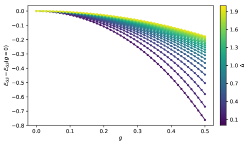
Figure 14: Dependence of the ground state energy with $g$ for several values of $\Delta$, for x = $5$ and $\epsilon=10^{-4}$. Solid lines represent results for the biased model. For comparison, dotted lines represent results for the unbiased model.

Appendix D Code

All numerical calculations can be found https://github.com/chuan97/TFG-Appendix-C.

References

- Roy et al. (2017) D. Roy, C. M. Wilson, and O. Firstenberg, Reviews of Modern Physics 89, 021001 (2017).
- Gu et al. (2017) X. Gu, A. F. Kockum, A. Miranowicz, Y.-x. Liu, and F. Nori, Physics Reports 718, 1 (2017).
- Astafiev et al. (2010) O. Astafiev, A. M. Zagoskin, A. Abdumalikov, Y. A. Pashkin, T. Yamamoto, K. Inomata, Y. Nakamura, and J. Tsai, Science 327, 840 (2010).
- Van Loo et al. (2013) A. F. Van Loo, A. Fedorov, K. Lalumière, B. C. Sanders, A. Blais, and A. Wallraff, Science 342, 1494 (2013).
- Liu and Houck (2017) Y. Liu and A. A. Houck, Nature Physics 13, 48 (2017).
- Faez et al. (2014) S. Faez, P. Türschmann, H. R. Haakh, S. Götzinger, and V. Sandoghdar, Physical review letters 113, 213601 (2014).
- Lodahl et al. (2015) P. Lodahl, S. Mahmoodian, and S. Stobbe, Reviews of Modern Physics 87, 347 (2015).
- Chang et al. (2018) D. Chang, J. Douglas, A. González-Tudela, C.-L. Hung, and H. Kimble, Reviews of Modern Physics 90, 031002 (2018).
- Argüello-Luengo et al. (2019) J. Argüello-Luengo, A. González-Tudela, T. Shi, P. Zoller, and J. I. Cirac, Nature 574, 215 (2019).
- Bello et al. (2019) M. Bello, G. Platero, J. I. Cirac, and A. González-Tudela, Science advances 5, eaaw0297 (2019).
- Lodahl et al. (2017) P. Lodahl, S. Mahmoodian, S. Stobbe, A. Rauschenbeutel, P. Schneeweiss, J. Volz, H. Pichler, and P. Zoller, Nature 541, 473 (2017).
- Sánchez-Burillo et al. (2019a) E. Sánchez-Burillo, C. Wan, D. Zueco, and A. González-Tudela, arXiv preprint arXiv:1907.00840 (2019a).
- Zheng et al. (2013) H. Zheng, D. J. Gauthier, and H. U. Baranger, Physical review letters 111, 090502 (2013).
- Niemczyk et al. (2010) T. Niemczyk, F. Deppe, H. Huebl, E. P. Menzel, F. Hocke, M. J. Schwarz, J. J. Garcia-Ripoll, D. Zueco, T. Hümmer, E. Solano, A. Marx, and R. Gross, Nature Physics 6, 772 (2010).
- Forn-Díaz et al. (2010) P. Forn-Díaz, J. Lisenfeld, D. Marcos, J. J. Garcia-Ripoll, E. Solano, C. Harmans, and J. Mooij, Physical review letters 105, 237001 (2010).
- Forn-Díaz et al. (2017) P. Forn-Díaz, J. J. García-Ripoll, B. Peropadre, J.-L. Orgiazzi, M. Yurtalan, R. Belyansky, C. M. Wilson, and A. Lupascu, Nature Physics 13, 39 (2017).
- Martínez et al. (2019) J. P. Martínez, S. Léger, N. Gheeraert, R. Dassonneville, L. Planat, F. Foroughi, Y. Krupko, O. Buisson, C. Naud, W. Hasch-Guichard, et al., npj Quantum Information 5, 19 (2019).
- Leger et al. (2019) S. Leger, J. Puertas-Martinez, K. Bharadwaj, R. Dassonneville, J. Delaforce, F. Foroughi, V. Milchakov, L. Planat, O. Buisson, C. Naud, W. Hasch-Guichard, S. Florens, I. Snyman, and N. Roch, arXiv preprint arXiv:1910.08340 (2019).
- Shirley (1965) J. H. Shirley, Physical Review 138, B979 (1965).
- Leggett et al. (1987) A. J. Leggett, S. Chakravarty, A. T. Dorsey, M. P. A. Fisher, A. Garg, and W. Zwerger, Reviews of Modern Physics 59, 1 (1987).
- Ashhab and Nori (2010) S. Ashhab and F. Nori, Physical Review A 81 (2010), 10.1103/physreva.81.042311.
- Ciuti et al. (2005) C. Ciuti, G. Bastard, and I. Carusotto, Phys. Rev. B 72, 115303 (2005).
- Stassi et al. (2013) R. Stassi, A. Ridolfo, O. D. Stefano, M. J. Hartmann, and S. Savasta, Physical Review Letters 110 (2013), 10.1103/physrevlett.110.243601.
- He et al. (2018) Q.-K. He, Z. An, H.-J. Song, and D. L. Zhou, ArXiv e-prints (2018), arXiv:1810.04523v1 .
- Liberato (2017) S. D. Liberato, Nature Communications 8 (2017), 10.1038/s41467-017-01504-5.
- Stassi et al. (2017) R. Stassi, V. Macrì, A. F. Kockum, O. D. Stefano, A. Miranowicz, S. Savasta, and F. Nori, Physical Review A 96 (2017), 10.1103/physreva.96.023818.
- Kockum et al. (2019) A. F. Kockum, A. Miranowicz, S. De Liberato, S. Savasta, and F. Nori, Nature Reviews Physics 1, 19 (2019).
- Forn-Díaz et al. (2019) P. Forn-Díaz, L. Lamata, E. Rico, J. Kono, and E. Solano, Reviews of Modern Physics 91, 025005 (2019).
- Peropadre et al. (2013) B. Peropadre, D. Zueco, D. Porras, and J. J. García-Ripoll, Physical review letters 111, 243602 (2013).
- Shi et al. (2018a) T. Shi, Y. Chang, and J. J. García-Ripoll, Physical Review Letters 120 (2018a), 10.1103/physrevlett.120.153602.
- Gheeraert et al. (2018) N. Gheeraert, X. H. Zhang, T. Sépulcre, S. Bera, N. Roch, H. U. Baranger, and S. Florens, Physical Review A 98, 043816 (2018).
- Sánchez-Burillo et al. (2014) E. Sánchez-Burillo, D. Zueco, J. Garcia-Ripoll, and L. Martin-Moreno, Physical review letters 113, 263604 (2014).
- Sánchez-Burillo et al. (2015) E. Sánchez-Burillo, J. García-Ripoll, L. Martín-Moreno, and D. Zueco, Faraday discussions 178, 335 (2015).
- Sánchez-Burillo et al. (2019b) E. Sánchez-Burillo, L. Martín-Moreno, J. García-Ripoll, and D. Zueco, Physical review letters 123, 013601 (2019b).
- Dzsotjan et al. (2011) D. Dzsotjan, J. Kästel, and M. Fleischhauer, Physical Review B 84, 075419 (2011).
- Gonzalez-Tudela et al. (2011) A. Gonzalez-Tudela, D. Martin-Cano, E. Moreno, L. Martin-Moreno, C. Tejedor, and F. J. Garcia-Vidal, Physical review letters 106, 020501 (2011).
- Zueco et al. (2012) D. Zueco, J. J. Mazo, E. Solano, and J. J. García-Ripoll, Physical Review B 86, 024503 (2012).
- Zheng and Baranger (2013) H. Zheng and H. U. Baranger, Physical review letters 110, 113601 (2013).
- Manzoni et al. (2017) M. T. Manzoni, L. Mathey, and D. E. Chang, Nature communications 8, 14696 (2017).
- John (1984) S. John, Phys. Rev. Lett. 53, 2169 (1984).
- John (1987) S. John, Phys. Rev. Lett. 58, 2486 (1987).
- John and Wang (1990) S. John and J. Wang, Physical review letters 64, 2418 (1990).
- John and Wang (1991) S. John and J. Wang, Phys. Rev. B 43, 12772 (1991).
- John and Quang (1994) S. John and T. Quang, Physical Review A 50, 1764 (1994).
- González-Tudela et al. (2015) A. González-Tudela, C.-L. Hung, D. E. Chang, J. I. Cirac, and H. J. Kimble, Nature Photonics 9, 320 (2015).
- Douglas et al. (2015) J. S. Douglas, H. Habibian, C.-L. Hung, A. V. Gorshkov, H. J. Kimble, and D. E. Chang, Nature Photonics 9, 326 (2015).
- Shi et al. (2016) T. Shi, Y.-H. Wu, A. González-Tudela, and J. I. Cirac, Physical Review X 6, 021027 (2016).
- Calajó et al. (2016) G. Calajó, F. Ciccarello, D. Chang, and P. Rabl, Physical Review A 93, 033833 (2016).
- González-Tudela and Cirac (2017a) A. González-Tudela and J. I. Cirac, Phys. Rev. A 96, 043811 (2017a).
- González-Tudela and Cirac (2017b) A. González-Tudela and J. I. Cirac, Phys. Rev. Lett. 119, 143602 (2017b).
- González-Tudela and Cirac (2018) A. González-Tudela and J. I. Cirac, Quantum 2, 97 (2018).
- González-Tudela and Cirac (2018) A. González-Tudela and J. I. Cirac, Phys. Rev. A 97, 043831 (2018).
- González-Tudela and Galve (2018) A. González-Tudela and F. Galve, ACS Photonics 6, 221 (2018).
- Shi et al. (2018b) T. Shi, Y. H. Wu, A. González-Tudela, and J. I. Cirac, New Journal of Physics 20, 105005 (2018b).
- Khalfin (1958) L. A. Khalfin, Soviet Physics JETP 6, 1053 (1958).
- Bykov (1975) V. P. Bykov, Soviet Journal of Quantum Electronics 4, 861 (1975).
- Fonda et al. (1978) L. Fonda, G. C. Ghirardi, and A. Rimini, Reports on Progress in Physics 41, 587 (1978).
- Onley and Kumar (1992) D. S. Onley and A. Kumar, American Journal of Physics 60, 432 (1992).
- Gaveau and Schulman (1995) B. Gaveau and L. Schulman, Journal of Physics A: Mathematical and General 28, 7359 (1995).
- Garmon et al. (2009) S. Garmon, H. Nakamura, N. Hatano, and T. Petrosky, Phys. Rev. B 80, 115318 (2009).
- Garmon et al. (2013) S. Garmon, T. Petrosky, L. Simine, and D. Segal, Fortschritte der Physik 61, 261 (2013).
- Garmon (2013) S. Garmon, in The Rochester Conferences on Coherence and Quantum Optics and the Quantum Information and Measurement meeting (OSA, 2013).
- Lombardo et al. (2014) F. Lombardo, F. Ciccarello, and G. M. Palma, Phys. Rev. A 89, 053826 (2014).
- Sánchez-Burillo et al. (2017) E. Sánchez-Burillo, D. Zueco, L. Martín-Moreno, and J. J. García-Ripoll, Physical Review A 96, 023831 (2017).
- Ulrich (1999) W. Ulrich, Quantum Dissipative Systems (Second Edition), Series In Modern Condensed Matter Physics (World Scientific Publishing Company, 1999).
- Prior et al. (2010) J. Prior, A. W. Chin, S. F. Huelga, and M. B. Plenio, Physical review letters 105, 050404 (2010).
- Grifoni and Hänggi (1998) M. Grifoni and P. Hänggi, Physics Reports 304, 229 (1998).
- Le Hur (2010) K. Le Hur, in Understanding Quantum Phase Transitions (CRC Press, 2010) pp. 245–268.
- Silbey and Harris (1984) R. Silbey and R. A. Harris, The Journal of chemical physics 80, 2615 (1984).
- Bera et al. (2014) S. Bera, A. Nazir, A. W. Chin, H. U. Baranger, and S. Florens, Physical Review B 90 (2014), 10.1103/physrevb.90.075110.
- Díaz-Camacho et al. (2016) G. Díaz-Camacho, A. Bermudez, and J. J. García-Ripoll, Phys. Rev. A 93, 043843 (2016).
- Zueco and García-Ripoll (2019) D. Zueco and J. García-Ripoll, Physical Review A 99, 013807 (2019).
- Shi et al. (2018c) T. Shi, E. Demler, and J. I. Cirac, Annals of Physics 390, 245 (2018c).
- Di Stefano et al. (2019) O. Di Stefano, A. Settineri, V. Macrì, L. Garziano, R. Stassi, S. Savasta, and F. Nori, Nature Physics , 1 (2019).
- Note (1) Take a function . Then, . This yields Eq. (6\@@italiccorr) in the main text.
- McCutcheon et al. (2010) D. P. S. McCutcheon, A. Nazir, S. Bose, and A. J. Fisher, Phys. Rev. B 81 (2010), 10.1103/physrevb.81.235321.
- Zheng et al. (2015) H. Zheng, Z. Lü, and Y. Zhao, Phys. Rev. E 91 (2015), 10.1103/physreve.91.062115.
- Guinea et al. (1998) F. Guinea, E. Bascones, and M. Calderon, in AIP Conference Proceedings, Vol. 438 (AIP, 1998) pp. 1–82.
- Note (2) For those who have condensed-matter background the spin-boson is paradigmatic in impurity models. In those formulations that naturally lead to a double-well interpretation of the TLS, the roles of and are switched in the Hamiltonian. In that case, is viewed as the delocalized regime whereas is viewed as the localized regime.
- Spohn1 and Domcke1 (1985) H. Spohn1 and R. Domcke1, Journal of Statistical Physics 41, 389 (1985).
- Löwen (1988) H. Löwen, Physical Review B 37, 8661 (1988).
- Novotny and Hecht (2006) L. Novotny and B. Hecht, Principles of Nano-Optics (Cambridge University Press, 2006).
- Longo et al. (2010) P. Longo, P. Schmitteckert, and K. Busch, Phys. Rev. Lett. 104, 023602 (2010).
- Longo et al. (2011) P. Longo, P. Schmitteckert, and K. Busch, Phys. Rev. A 83, 063828 (2011).
- Sánchez-Burillo et al. (2018) E. Sánchez-Burillo, A. Cadarso, L. Martín-Moreno, J. J. García-Ripoll, and D. Zueco, New Journal of Physics 20, 013017 (2018).
- Note (3) To exemplify the weakness of the dipole-dipole interaction, it is insightful to remember that it was not strong enough to explain ferromagnetism in solids. The exchange interaction had to be introduced in the study of ferromagnetism for this very reason.