Coupled Möbius Maps as a Tool to Model Kuramoto Phase Synchronization

Abstract

We propose Möbius maps as a tool to model synchronization phenomena in coupled phase oscillators. Not only does the map provide fast computation of phase synchronization, it also reflects the underlying group structure of the sinusoidally coupled continuous phase dynamics. We study map versions of various known continuous-time collective dynamics, such as the synchronization transition in the Kuramoto-Sakaguchi model of non-identical oscillators, chimeras in two coupled populations of identical phase oscillators, and Kuramoto-Battogtokh chimeras on a ring, and demonstrate similarities and differences between the iterated map models and their known continuous-time counterparts.

I Introduction

Ensembles of sinusoidally coupled phase oscillators Kuramoto (1975); Pazó and Montbrió (2014) are widely adopted as canonical models for synchronization in various scientific and engineering inquiries. For instance, models of coupled phase oscillators have been successfully applied to functional connectivity of the human brain Cabral et al. (2011); Petkoski et al. (2018), neuronal oscillatory behavior Breakspear et al. (2010); Montbrió and Pazó (2018), and neural encoding Doesburg et al. (2009); Malagarriga et al. (2015); Soman et al. (2018). Increasingly, they also serve as a computational tool in machine learning and artificial intelligence based on oscillatory neural networks Hoppensteadt and Izhikevich (2000); Chakraborty et al. (2014); Vodenicarevic et al. (2016); Zhang et al. (2019), which opens up a new perspective for hardware implementations Heger and Krischer (2016).

The most popular models in the field, the Kuramoto-Sakaguchi model Sakaguchi and Kuramoto (1986) and the Winfree model Winfree (1967) are formulated as systems of ordinary differential equations for coupled phase oscillators. The goal of this paper is to formulate a discrete-time analogue of the Kuramoto-Sakaguchi model as a system of coupled maps, that has similar dynamical properties but provides a fast computation of the dynamics in discrete-time steps.

Globally coupled maps Kaneko (1990, 1991); Nozawa (1992); Pikovsky and Kurths (1994); Just (1995); Topaj et al. (2001) have been intensively studied in the literature, often with emphasis on the collective dynamics of intrinsically chaotic units. Among the existing map models, coupled circle maps are ideal for studying synchronization phenomena due to their periodic domains. The simplest and most widely used circle map is the sine circle map $\varphi\to\varphi+\Omega+\varepsilon\sin\varphi$, which has been explored in the context of global coupling Kaneko (1991); Chatterjee and Gupte (1996); Osipov and Kurths (2002) as well as in non-trivial coupling networks such as computational neural networks Bauer and Martienssen (2009). However, the coupled sine circle maps have several properties different from that of the Kuramoto-Sakaguchi model. For example, a known property of the continuous-time Kuramoto-Sakaguchi model is that clustering, i.e., the formation of several distinct synchronized groups, cannot occur Gong et al. (2019). However, for the sine circle maps, even though the map parameters can be tuned to certain regions such that no chaos is produced by the iteration of a single map (i.e., the mapping remains one-to-one), the coupled iterated map dynamics of identical units governed by the same mean field nevertheless produces various complex cluster states.

As shown in previous literature, the propagator of continuous-time phase oscillators forced proportionally to the first harmonics of the phase has the form of a Möbius transformation Marvel et al. (2009). The Möbius transform lies at the heart of the low-dimensional dynamical theory for globally forced populations of continuous-time phase oscillators formulated by Watanabe and Strogatz (WS) Watanabe and Strogatz (1994); Pikovsky and Rosenblum (2008); Marvel et al. (2009); Pikovsky and Rosenblum (2015); Chen et al. (2017). There, the Möbius transform is used to convert the original phase variables to new conserved quantities, such that the time-varying transformation parameters obey a simple low-dimensional system of ordinary differential equations.

In this paper, we implement a Möbius map, inspired from the aforementioned Möbius transform, as the basic circle map. The main arguments for studying synchronization and collective dynamics using Möbius maps are threefold. First, similar to the solution of a continuous-time Kuramoto-type phase model, an ensemble of infinite units governed by Möbius maps possesses a low-dimensional manifold (corresponding to the Ott-Antonsen (OA) manifold Ott and Antonsen (2008) for continuous-time oscillators). Therefore, the equation for the mean field can be reduced to a low-dimensional map, whereas the mean-field equations for more general circle maps are generic infinite-dimensional nonlinear Perron-Frobenius operators. One exception is homographic maps Griniasty and Hakim (1994), which as we will discuss in Section II.3 below, are equivalent to Möbius maps. Secondly, iterated maps allow for large changes of the system state at each time step, in contrast to numerical integration of ordinary differential equations (ODEs) – a property which can be exploited to speed up computation for large systems. Third, while Möbius maps can fully reproduce the ODE behaviour within certain limit of map parameters, new and interesting dynamics is also possible, e.g. for strong negative coupling.

The plan of the paper is as follows. In Sec. II, we first review the general form of the complex Möbius map and discuss its group properties. We discuss its single-map dynamics under function iteration and fixed parameters. Next, by allowing the parameters of the map to vary in time and applying the group properties, we study the low-dimensional dynamics in globally coupled identical maps, and make the connection to the WS and OA mean-field reduction theories. Finally, we give a real-valued representation of the Möbius map on the unit circle to be used in numerical calculations and remark on a connection of the theory of Möbius maps with earlier results for homographic maps. In Sec. III we give a compact expression of the Möbius map which solves the Adler equation for phase dynamics on an arbitrary time interval. In Sec. IV, we use this result to construct a map model of globally coupled, non-identical oscillators, as a discrete-time counterpart to the Kuramoto-Sakaguchi model Sakaguchi and Kuramoto (1986). We discuss the dynamics of globally coupled Möbius maps with frequency heterogeneity, of chimera states in two populations of identical phase oscillators with different intra- and inter-population couplings Abrams et al. (2008), and of chimeras on a periodic lattice of identical oscillators with non-local coupling Abrams and Strogatz (2004); Kuramoto and Battogtokh (2002); Kalle et al. (2017). In all examples, known behaviours of the continuous-time dynamics can be reproduced qualitatively under positive coupling, and an interesting new synchronizing behaviour can be found for finite negative coupling, under which the familiar continuous-time dynamics would simply be incoherent or asynchronous.

II Möbius map and its properties

In this section we heavily rely on the excellent introduction of Möbius transformation and Möbius group in the context of continuous-time dynamics by Marvel, Mirollo, and Strogatz Marvel et al. (2009). We will repeat some results from Ref. Marvel et al. (2009) for the sake of consistency. Our extension of Ref. Marvel et al. (2009) is the introduction of the Möbius circle map as a dynamical system (Section II.1), and the formulation of the low-dimensional discrete-time equations governing the evolution of ensembles (Section II.2). Additionally, we give a real-valued representation of the map on the complex unit circle and connect the Möbius maps to homographic maps on the real line, where low-dimensional mean-field behavior on an invariant manifold for infinite ensembles has been reported previously Griniasty and Hakim (1994).

II.1 Standard form and dynamics of a single iterated map

For the Möbius transformation we use the same parametrization as in Ref. Marvel et al. (2009)

$$\mathcal{M}_{q,\psi}\left(z\right)=\frac{q+e^{i\psi}z}{1+q^{*}e^{i\psi}z}~{},$$ (1)

with parameters $(q,\psi)\in\mathbb{D}\times S^{1}$, where $|q|<1$, i.e., $q$ is on the open complex unit disc $\mathbb{D}$, and $\exp(i\psi)\in S^{1}$ on the complex unit circle $S^{1}$. The complex conjugate of $q$ is denoted as $q^{*}$. Transformation (1) can be applied to any complex number $z$ in the closed unit disk, $z\in\{\mathbb{D}\cup S^{1}\}$. Transformation (1) is invertible and leaves the complex unit circle invariant. This property will be used to define a circle map. Möbius transformation (1) can be decomposed as two independent actions

$$\mathcal{M}_{q,\psi}\left(z\right)=\mathcal{C}_{q}\circ\mathcal{R}_{\psi}\left(z\right)~{},$$ (2)

where $\mathcal{R}_{\psi}$ denotes rotation by an angle $\psi$

$$\mathcal{R}_{\psi}:z\to e^{i\psi}z~{},$$ (3)

and $\mathcal{C}_{q}$ denotes a directional contraction

$$\mathcal{C}_{q}:z\to\frac{q+z}{1+q^{*}z}~{}.$$ (4)

The identity transformation is $\mathcal{M}_{0,0}$. The rotational actions commute: $\mathcal{R}_{\psi_{1}}\circ\mathcal{R}_{\psi_{2}}=\mathcal{R}_{\psi_{2}}\circ\mathcal{R}_{\psi_{1}}=\mathcal{R}_{\psi_{1}+\psi_{2}}$, with the inverse of the rotation $\mathcal{R}^{-1}_{\psi}=\mathcal{R}_{-\psi}$. The inverse of the contraction is $\mathcal{C}_{q}^{-1}=\mathcal{C}_{-q}$ such that

$$\mathcal{M}^{-1}_{q,\psi}=\mathcal{R}_{-\psi}\circ\mathcal{C}_{-q}~{}.$$ (5)

Rotational symmetry is expressed as

$$\mathcal{C}_{q}=\mathcal{R}_{-\psi}\circ\mathcal{C}_{qe^{i\psi}}\circ\mathcal{R}_{\psi}~{}.$$ (6)

It is well known that Möbius transformation forms a group under functional composition

$$\mathcal{M}_{q_{2},\psi_{2}}\left(z\right)=\mathcal{M}_{q_{1},\psi_{1}}\circ\mathcal{M}_{q_{0},\psi_{0}}\left(z\right)~{}.$$ (7)

This is to say, the group parameters $q_{2},\psi_{2}$ of the new transformation are functions of the parameters of the component transformations. Under parametrization (1), these functions are (see Appendix A for a detailed derivation):

$$q_{2}=\mathcal{M}_{q_{1},\psi_{1}}\left(q_{0}\right)\;,\quad e^{i\psi_{2}}=\mathcal{C}_{q_{1}q^{*}_{0}}\left(e^{i\psi_{1}}\right)\cdot e^{i\psi_{0}}\;.$$ (8)

We now consider a complex variable $z=e^{i\varphi}$ on the unit circle, and define a Möbius circle map by virtue of the transformation (1):

$$e^{i\varphi^{(n+1)}}=\mathcal{M}_{q,\psi}\left(e^{i\varphi^{(n)}}\right)\;,$$ (9)

where $n=0,1,\ldots$ is a discrete time index. Map $\mathcal{M}_{q,\psi}$ is defined by a complex parameter $q=\rho\exp(i\vartheta)$ and a real parameter $\psi$. Here we first assume the parameters $q,\psi$ to be constant.

Circle map (9), contrary to generic smooth circle maps, possesses a very simple dynamics under iteration. It can be shown that it has just one Arnold tongue – a region of synchronous phase locking with rotation number zero, while tongues with other rotation numbers do not exist. This should be contrasted with the existence of Arnold tongues with all rational rotation numbers for generic circle maps Katok and Hasselblatt (1995). The rotation number $\eta$ can be defined according to Refs. Katok and Hasselblatt (1995); Pikovsky et al. (2001) as

$$\eta=\lim_{n\to\infty}\frac{\varphi^{(n)}-\varphi^{(0)}}{2\pi n}~{},$$ (10)

where the phase variable is lifted to the real line. Derived in detail in Appendix B, the rotation number of map (9) can be expressed as

$$\eta=\begin{cases}0&\text{for}\quad\rho>\left|\sin\frac{\psi}{2}\right|\;,\\ \frac{1}{\pi}\arctan\left(\tan\frac{\psi}{2}\cdot\sqrt{1-\frac{\rho^{2}}{\sin^{2}\frac{\psi}{2}}}\right)&\quad\textrm{otherwise.}\end{cases}$$ (11)

The rotation number of the Möbius map as a function of parameter $\psi$ is demonstrated in Fig. 1, where numerical and analytical results are shown to coincide. One can see a plateau with $\eta=0$ for $\rho>\left|\sin\frac{\psi}{2}\right|$ and smooth dependence on $\psi$ outside the plateau. In the domain $\eta\neq 0$, as is derived in Appendix B, the Möbius map is conjugate (by virtue of another Möbius transformation) to a circle shift.

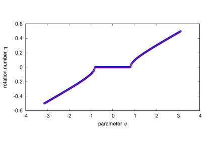
Figure 1: The rotation number $\eta$ of iterated Möbius maps as a function of map parameter $\psi$, given $\rho=0.4$. Open circles: direct numerical simulations; solid line: formula (11).

The above calculation consists an analytical proof for the existence of one single Arnold tongue in iterated dynamics of Möbius maps of fixed parameters. Another way of proving the same result is by considering the group property of Möbius map (7). If we assume to the contrary, that Möbius map (9) under iteration has an Arnold tongue with a non-integer rotation number, then it follows that there exists a stable periodic orbit with a period larger than one. This in turn implies that an iteration over such a period results in several stable fixed points. But from the group property (7), we know that any iteration of the Möbius map is again a Möbius map, and a Möbius map can have at most only one stable fixed point. This contradicts the assumption that Möbius map (9) has an Arnold tongue with a non-integer rotation number. Hence Möbius map (9) can only possess Arnold tongues of integer rotation number.

This special property of Möbius maps having only one Arnold tongue has another consequence, namely, that different phases iterated by the same Möbius map may form at most one cluster. A cluster $K\{\varphi^{(n)}_{j},j=1\dots N\}$ is a subset of phases in an ensemble which contract to a single point on the unit circle in the course of the phase evolution, i.e., $\lim_{n\to\infty}\exp[i(\varphi_{k}^{(n)}-\varphi_{j}^{(n)})]=1$ for all pairs of phases $\{\varphi_{k},\varphi_{j}\}$ in the cluster. Since the evolution of any phase variable $\varphi^{(0)}\to\varphi^{(n)}$ is given by the same Möbius map, which has at most one attractive fixed point, only one cluster can be formed under a common iterated Möbius map of fixed or time-varying parameters, with the possible exception of one phase located precisely at the unstable fixed point of the map, outside the cluster.

Under the iteration of Möbius maps, as with all invertible circle maps, chaotic dynamics of the phases cannot occur, regardless of whether the map parameters are constant, time-varying, or follow chaotic sequences.

II.2 Low-dimensional evolution of oscillator ensembles under Möbius maps

The group property of the Möbius maps, as shown by Eqs. (7) and (8), implies that the evolution under Möbius map dynamics (9) from any set of initial states is reducible to a three-dimensional evolution of the map parameters $q$ and $\psi$. To see this, consider the single-map dynamics (9) with an arbitrary discrete sequence of parameters $q^{(n)},\psi^{(n)}$ that vary in time

$$e^{i\varphi^{(n)}}=\mathcal{M}_{q^{(n)},\psi^{(n)}}\left(e^{i\varphi^{(n-1)}}\right)\;.$$ (12)

Due to the group property (7), the evolution over any time interval from the initial state $\exp(i\varphi^{(0)})$ to the final state $\exp(i\varphi^{(n)})$ can also be expressed as a Möbius map

$$e^{i\varphi^{(n)}}=\mathcal{M}_{Q^{(n)},\Psi^{(n)}}\left(e^{i\varphi^{(0)}}\right).$$ (13)

Shifting $n\to(n-1)$, applying map (12) of time step $n$ to both sides of (13) and using the transformation rule (8) for composite group parameters, we obtain the evolution equations of $Q$ and $\Psi$

$$Q^{(n)} =\mathcal{M}_{q^{(n)},\psi^{(n)}}\left(Q^{(n-1)}\right)~{},$$ (14)

$$e^{i\Psi^{(n)}} =\mathcal{C}_{q^{(n)}Q^{*(n-1)}}\left(e^{i\psi^{(n)}}\right)e^{i\Psi^{(n-1)}}~{}.$$

The initial values $Q^{(0)}=0$ and $\Psi^{(0)}=0$ follow from the identity map $\mathcal{M}_{0,0}(z)=z$.

We note that the transformation governing $Q$ is the same as the original Möbius map (12) for the phase $\varphi$, but here it is applied to a complex variable defined on the unit disc, and not on the unit circle.

Because transformation (14) does not depend on the initial phase $\varphi^{(0)}$, it can be used to describe the evolution of any initial state of the phase by first applying the map (14) for $Q^{(n)}$ and then applying the map (13) for the phase. Thus, the evolution of any ensemble of oscillators by a sequence of Möbius maps is always restricted to a three-dimensional manifold described by (14) and parametrized by $(Q^{(n)},\Psi^{(n)})\in\mathbb{D}\times S^{1}$. Hence, the discrete-time dynamics (14) for an ensemble of oscillators under common forcing is fully analogous to the Watanabe-Strogatz quasi-mean-field equations in the continuous-time case Watanabe and Strogatz (1994). The role of the three-dimensional manifold is the same as in the continuous-time case: It implies that for any number of units, the dynamics can be split into constants of motion (e.g., initial values of the phases) and three dynamical variables $(Q^{(n)},\Psi^{(n)})$, the evolution of which may be nontrivial. One often calls this property of the phase dynamics “partial integrability”.

Even for an infinite ensemble of oscillators described by a density $\mu(\varphi)$, the evolution takes place on a three-dimensional invariant manifold. $\mu_{Q,\Psi}(\varphi)$ denotes the density of oscillator phases after the transformation $\exp(i\varphi)\to\mathcal{M}_{Q,\Psi}(\exp(i\varphi))$ from an initial density $\mu_{0,0}(\varphi)$. The family of densities $\mu_{Q,\Psi}(\varphi)$ is a three-dimensional invariant manifold, parametrized by $Q$ and $\Psi$. In the special case of a continuous, uniform phase density $\mu_{0,0}(\varphi)=1/(2\pi)$, the resulting family of densities $\mu_{Q,\Psi}(\varphi)=\mu_{Q}(\varphi)$ is independent of $\Psi$, which corresponds to an angular shift that leaves the uniform density invariant on the circle. As shown in Ref. Marvel et al. (2009) and Appendix C, $\mu_{Q}(\varphi)$ is the family of wrapped Cauchy distributions

$$\mu_{Q}(\varphi)=\frac{1}{2\pi}\frac{1-|Q|^{2}}{|e^{i\varphi}-Q|^{2}}\;.$$ (15)

This family of phase densities is called the Ott-Antonsen (OA) manifold in continuous-time phase dynamics Ott and Antonsen (2008), and we shall use the same name to discuss the manifold in the map dynamics here. On the OA manifold, the Kuramoto mean field $Z=\left\langle\exp(i\varphi)\right\rangle_{\mu_{Q}}$ is in fact identical to the Möbius map parameter $Q$ (Appendix C). Replacing map parameter $Q$ with the mean field $Z$ in (14), it follows that the exact evolution of the ensemble mean field can also be expressed as an iterated Möbius transformation

$$Z^{(n)}=\mathcal{M}_{q^{(n)},\psi^{(n)}}\left(Z^{(n-1)}\right)=\frac{q^{(n)}+e^{i\psi^{(n)}}Z^{(n-1)}}{1+q^{*(n)}e^{i\psi^{(n)}}Z^{(n-1)}}\;.\quad$$ (16)

It is interesting to note that, the map for the mean field (16) has exactly the same form as the map describing the dynamics (12) of every single oscillator in the ensemble. However, the domains of the two maps differ: while the complex oscillators $\exp(i\varphi)$ are always on the unit circle, the mean field $Z$ is an element of the unit disc, i.e. $|Z|\leq 1$.

As a side note, the sequences $q^{(n)}$ and $\psi^{(n)}$ in Eq. (12) are arbitrary and may be functions of $Z$ or contain random components. In this way, more complicated noisy dynamics and globally coupled oscillators can also be studied with the discrete map model proposed here for which all the results above still hold.

II.3 Real-valued representation and relation to homographic maps

For computational purposes, an equivalent form of parametrization of the Möbius map may be used, which is more suited for programming languages that do not natively support a data type for complex numbers. Using identity $\exp(is)=(1+i\tan\frac{s}{2})(1-i\tan\frac{s}{2})^{-1}$ and $q=\rho\exp(i\vartheta)$ as before, we can rewrite (9) in the trigonometric form

$$\tan\frac{\varphi^{(n+1)}-\vartheta}{2}=\frac{1-\rho}{1+\rho}\tan\frac{\varphi^{(n)}+\psi-\vartheta}{2}~{}.$$ (17)

Manipulating (17) we then obtain the computationally simple Möbius map via the ATAN2 function

$$\begin{gathered}\varphi^{(n+1)}=\vartheta+\text{ATAN2}\left[(1-\rho^{2})\sin(\varphi^{(n)}+\psi-\vartheta),\right.\\ \left.(1+\rho^{2})\cos(\varphi^{(n)}+\psi-\vartheta)+2\rho\right]\;.\end{gathered}$$ (18)

Griniasty and Hakim Griniasty and Hakim (1994) studied a family of homographic maps, defined for real variable $x$ as

$$x^{(n+1)}=a-\frac{b}{x^{(n)}}\;.$$ (19)

This map leaves a Cauchy distribution invariant, in the same way that Möbius maps leave a wrapped Cauchy distribution invariant. The homographic map (19) can be shown to be equivalent to a Möbius map. Indeed, by a substitution $x^{(n)}=\tan{(\varphi^{(n)}/2)}=i(1-e^{i\varphi^{(n)}})(1+e^{i\varphi^{(n)}})^{-1}$ we can rewrite (19) as the Möbius map (9) for $\varphi^{(n)}$ with parameters

$$q=\frac{i(1-b)+a}{i(1+b)+a},\quad e^{i\psi}=\frac{a-i(1+b)}{a+i(1+b)}\;.$$ (20)

Given a Cauchy distribution with mean $r$ and scale parameter $s$, the complex number $z=r+is$ can be shown to be transformed under the same homographic map $z^{(n+1)}=a-b/z^{(n)}$ as the Cauchy distributed variables $x^{(n)}$. This is to say, that the low-dimensional reduction for ensembles evolved under iterated homographic maps was already deduced in Griniasty and Hakim (1994), almost at the same time as the discovery of the low-dimensional dynamics in the ensembles of phase oscillators Watanabe and Strogatz (1994); Ott and Antonsen (2008); Marvel et al. (2009).

III Relation to Adler equation

Many continuous-time phase models of coupled oscillators can be written in the form of an Adler equation Adler (1946) with constant or time-varying parameters. As we shall see, the solution of the Adler equation has the form of a Möbius map. This allows us to build Möbius map models of coupled oscillators analogous to continuous-time models. In this section we relate the parameters of the Adler equation to those of the Möbius map.

The Adler equation with constant parameters can be written in the form

$$\dot{\varphi}=A\left[\lambda-\sin(\varphi-\beta)\right]~{},$$ (21)

where the real-valued parameters consist of the amplitude $A$, the ratio $\lambda$ between the constant bias term and the amplitude of the sinusoidal forcing, and the phase shift $\beta$. It is known that for $|\lambda|\leq 1$ the Adler equation has a steady state solution, and for $|\lambda|>1$, it yields phase rotations.

The solution of the Adler equation with fixed parameters $A,\lambda,\beta$ over a time interval $\tau$ can be shown to be a Möbius map (see Appendix D for details). Here $A$ and $\tau$ only enter the solution as a product $P=A\tau$. Denoting

$$\sigma=\sqrt{1-\lambda^{2}},\quad\Gamma=\tanh\left(\frac{P}{2}\sigma\right)~{},$$ (22)

and using the conventions $\sqrt{-1}=i$ and $\tanh(ix)=i\tan(x)$, we can write the solution of the Adler equation as the Möbius map

$$e^{i\varphi(\tau)}=\frac{(\sigma+i\lambda\Gamma)e^{i\varphi(0)}+e^{i\beta}\Gamma}{(\sigma-i\lambda\Gamma)+e^{i\varphi(0)}e^{-i\beta}\Gamma}=\mathcal{M}_{q,\psi}\left(e^{i\varphi(0)}\right)$$ (23)

with group parameters

$$q=e^{i\beta}\frac{\Gamma}{\sigma-i\lambda\Gamma}~{},\qquad e^{i\psi}=\frac{\sigma+i\lambda\Gamma}{\sigma-i\lambda\Gamma}~{}.$$ (24)

The saddle-node bifurcation for the Adler equation at $|\lambda|=1$ corresponds to the tangent bifurcation of the circle map. At the bifurcation, Eqs. (24) need to be evaluated in the limit $\lambda\to\pm 1$, i.e.,

$$q=e^{i\beta}\frac{P}{2\mp iP}~{},\qquad e^{i\psi}=\frac{2\pm iP}{2\mp iP}~{}.$$ (25)

If the solution to the Adler equation after interval $\tau$ is a Möbius map, then the evolution under iterated Möbius maps is a Möbius map again, as shown by the group property in Sec. II. Therefore, taking infinitesimal time steps, the solution of the Adler equation with time dependent parameters $A(t)$, $\lambda(t)$ and $\beta(t)$ is still a Möbius map.

Consequently, all basic properties of the Adler equation are inherited by the Möbius map. In particular, it is known that for a solution to the Adler equation which has a periodic dependence on its parameters, there is only one Arnold tongue for every integer rotation number Buchstaber et al. (2010); Ilyashenko et al. (2011). This matches exactly the property of Möbius map as discussed in Section II, i.e. the Möbius map has at most one stable fixed point in the synchronized state. Hence, Eq. (23) can be viewed as a numerical scheme to simulate the continuous-time Adler equation with small time step $\tau$. In fact, while a standard Euler scheme, which to the linear order in $\tau$ coincides with the Möbius map, breaks the Watanabe-Strogatz partial integrability of the Adler equation Gong et al. (2019), the Möbius map (23) preserves this partial integrability, similar to the symplectic integration schemes for Hamiltonian equations. Because the map keeps the properties of the Adler equation also for large $\tau$, it offers a possibility to model features of oscillators obeying the Adler-type dynamics with an increased computational efficiency, even though the main bottleneck of computing the mean-field at each step remains for coupled maps (see Appendix E for more details).

In the special case where only the amplitude $A=A(t)$ has explicit time dependence, the Adler equation (21) has the form of a phase response to a time-dependent forcing, $\dot{\varphi}=H(\varphi)A(t)$. The exact solution of (21) in this case can be obtained by separation of variables. The solution has the same form as (22) and (23), except in this case the parameter $P$ is the integral of $A(t)$ over the time interval $\tau$

$$P=\int_{0}^{\tau}A(t)dt~{}.$$ (26)

Here, the time-dependent kick amplitude $A(t)$ can be any generic function, e.g. a delta pulse or a constant force.

IV Mean-Field Dynamics for Phases Evolved Under Coupled Möbius Maps

IV.1 Formulation of a model of globally coupled maps with Kuramoto-Sakaguchi-type coupling

The Kuramoto-Sakaguchi model of globally coupled phase oscillators is formulated as a system of $N$ Adler-type equations

$$\dot{\varphi}_{j}=\omega_{j}+\varepsilon R\sin(\Theta-\varphi_{j}-\alpha)~{},$$ (27)

where the forcing, common to all oscillators, is expressed through the complex mean field

$$Z=Re^{i\Theta}=\frac{1}{N}\sum_{j=1}^{N}e^{i\varphi_{j}}=\langle e^{i\varphi_{j}}\rangle_{j}~{}.$$ (28)

Here, natural frequencies $\omega_{j}$ can be typically assumed to be sampled from some distribution. In this section, we build a discrete analogue of model (27) based on the Möbius maps.

Comparing (27) with the Adler equation (21), one can see that $A$ corresponds to $\varepsilon R$, $\beta$ corresponds to $\Theta-\alpha$, and $\lambda$ corresponds to $\omega_{j}/(\varepsilon R)$. However, a direct application of the map solution (23) of the discrete-time Adler equation is not optimal here, because parameters $\lambda$ and $A$ enter (23) in a rather complex manner. In order to obtain a simple discrete-time model, which not only carries the essential properties of a globally forced continuous-time phase model, but also allows an analytic evaluation of averages with respect to some distribution of natural frequencies, we split the phase evolution in the Kuramoto-Sakaguchi model into two stages. In the first stage a delta pulse of strength $P^{(n)}=\varepsilon R^{(n)}$ is applied to all oscillators, the solution to which corresponds to (23) with $\beta^{(n)}=\Theta^{(n)}-\alpha$ and $\lambda=0$. Here $R^{(n)}\exp(i\Theta^{(n)})$ is the mean field calculated just prior to the kick by the delta pulse. In the second stage, the oscillators undergo free rotation for a time interval $T$ with individual natural frequencies $\omega_{j}$. This stage corresponds to the map $\varphi_{j}\to\varphi_{j}+\omega_{j}T$. Combining stages one and two, we formulate the resulting model of heterogeneous, globally coupled oscillators as

$$e^{i\varphi_{j}^{(n+1)}}=e^{i\omega_{j}T}\frac{e^{i\varphi_{j}^{(n)}}+e^{i\Theta^{(n)}-i\alpha}\tanh\frac{\varepsilon R^{(n)}}{2}}{1+e^{i\varphi_{j}^{(n)}}e^{-i\Theta^{(n)}+i\alpha}\tanh\frac{\varepsilon R^{(n)}}{2}}\;.$$ (29)

Here the mean field is defined as

$$R^{(n)}e^{i\Theta^{(n)}}=\frac{1}{N}\sum_{j=1}^{N}e^{i\varphi_{j}^{(n)}}\;.$$ (30)

Taking $T\to dt$ and $\varepsilon\to\varepsilon dt$ the map (29) is to the linear order in $dt$ equivalent to an Euler integration step for the continuous-time Kuramoto-Sakaguchi model (27) and solves the ODE exactly in the limit $dt\to 0$. In the thermodynamic limit and on the Ott-Antonsen manifold, the phase density $\mu_{Q}(\varphi,\omega)$ for each value of frequency $\omega$ is a wrapped Cauchy distribution with mean field $Q(\omega)=\left\langle e^{i\varphi}\right\rangle_{\mu_{Q}(\varphi,\omega)}$, as shown above in Sec. II.2. According to (16), parameter $Q$ then obeys the same map as the individual phases having natural frequency $\omega$ (29), i.e.

$$Q^{(n+1)}(\omega)=e^{i\omega T}\frac{Q^{(n)}(\omega)+e^{i(\Theta^{(n)}-\alpha)}\tanh\frac{\varepsilon R^{(n)}}{2}}{1+Q^{(n)}(\omega)e^{-i(\Theta^{(n)}-\alpha)}\tanh\frac{\varepsilon R^{(n)}}{2}}~{}.$$ (31)

The value of the mean field $Z$ can be calculated as the average of $Q^{(n)}(\omega)$ with respect to a continuous distribution density of natural frequencies $g(\omega)$

$$Z^{(n)}=R^{(n)}e^{i\Theta^{(n)}}=\int_{-\infty}^{\infty}Q^{(n)}(\omega)g(\omega)d\omega~{}.$$ (32)

Similar to the approach of Ott and Antonsen Ott and Antonsen (2008), we can assume that $Q(\omega)$ is analytic in the upper half-plane, which allows us to calculate the integral via the residue theorem. For a Lorentzian frequency distribution of mean $\omega_{0}$ and scale parameter $\gamma$

$$g(\omega)=\frac{1}{\pi\gamma}\frac{\gamma^{2}}{(\omega-\omega_{0})^{2}+\gamma^{2}}~{},$$ (33)

the mean field is $Z=Q(\omega_{0}+i\gamma)$. Accordingly, the global mean field evolves according to the following map

$$Z^{(n+1)}=e^{(i\omega_{0}-\gamma)T}\frac{Z^{(n)}+e^{i(\Theta^{(n)}-\alpha)}\tanh\left(\frac{\varepsilon R^{(n)}}{2}\right)}{1+Z^{(n)}e^{-i(\Theta^{(n)}-\alpha)}\tanh\left(\frac{\varepsilon R^{(n)}}{2}\right)}~{}.$$ (34)

The first part of map (34), $e^{(i\omega_{0}-\gamma)T}$, consists of a rotation with the mean frequency $\omega_{0}$ of the ensemble, and a decay of the mean field due to population heterogeneity $\gamma$, which is determined by the width of the natural frequency distribution. Equation (34) is a discrete analogue of the Ott-Antonsen equation Ott and Antonsen (2008) which describes the dynamics of the mean field in the Kuramoto-Sakaguchi model.

For globally coupled Möbius maps we can calculate the steady state order parameter $\tilde{R}=R\exp(\gamma T)$ after each kick implicitly. Because we can always go into the co-rotating frame with the mean frequency $\omega_{0}$, we can set it to 0 without loss of generality. Setting the order parameter $\tilde{R}$ equal on both sides of (34)

$$\begin{gathered}\tilde{R}^{2}=\left|\frac{\Gamma e^{-i\alpha}+\tilde{R}e^{-\gamma T}}{1+\Gamma e^{i\alpha}\tilde{R}e^{-\gamma T}}\right|^{2}=\\ =\frac{\Gamma^{2}+\tilde{R}^{2}e^{-2\gamma T}+2\Gamma\tilde{R}e^{-\gamma T}\cos\alpha}{1+\Gamma^{2}\tilde{R}^{2}e^{-2\gamma T}+2\Gamma\tilde{R}e^{-\gamma T}\cos\alpha}\;,\end{gathered}$$ (35)

where $\Gamma=\tanh\left(\varepsilon e^{-\gamma T}\tilde{R}/2\right)$, we solve a quadratic equation for $\Gamma$, and obtain

$$\Gamma=\frac{\tilde{R}}{1-\tilde{R}^{4}e^{-2\gamma T}}\left[-(1-\tilde{R}^{2})e^{-\gamma T}\cos\alpha\right.$$ (36)

$$\left.\pm\sqrt{(1-\tilde{R}^{2})^{2}e^{-2\gamma T}\cos^{2}\alpha+\left(1-e^{-2\gamma T}\right)\left(1-\tilde{R}^{4}e^{-2\gamma T}\right)}\right]~{}.$$

Inverting the expression for $\varepsilon$ we obtain

$$\varepsilon=\frac{2}{\tilde{R}e^{-\gamma T}}\textrm{arctanh}\left(\Gamma\right)~{}.$$ (37)

Eq. (36) and Eq. (37) together allow us to express coupling strength $\varepsilon$ explicitly as a function of the steady state synchronization order parameter $\tilde{R}$ and to plot them in a bifurcation diagram, as shown in Fig. 2..

The first notable limit of the expression of the bifurcation curve is the existence of two critical coupling strengths for $\tilde{R}\to 0$

$$\varepsilon_{cr}=2\left(-\cos\alpha\pm\sqrt{\cos^{2}\alpha+e^{2\gamma T}-1}\right)~{}.$$ (38)

Eq. (38) implies that there is always a positive and a negative critical coupling strength for the incoherent state in globally coupled Möbius maps. The second limit is the limit of identical oscillators $\gamma\to 0$, in which case $\tilde{R}=R$ and

$$\Gamma=\tanh\left(\frac{\varepsilon R}{2}\right)=R\frac{-\cos\alpha\pm\left|\cos\alpha\right|}{1+R^{2}}~{}.$$ (39)

Eq. (39) indicates the existence of two lines of fixed points connecting incoherence at $R=0$ and complete synchronization at $R=1$, for a given value of $\alpha$.

Under negative coupling and identical frequency, there are several regimes for a transition to synchrony. At $\varepsilon_{0}=0$, the stability of complete synchronization and incoherence is exchanged instantly. At $\varepsilon_{1}=-4\cos\alpha$, incoherence at $R=0$ becomes unstable, and at $\varepsilon_{2}=\ln\left[(1-\cos\alpha)/(1+\cos\alpha)\right]$, complete synchronization at $R=1$ becomes unstable.

The existence of a synchronization transition for strongly repulsively coupled oscillators under discrete time stands in stark contrast to the continuous-time Kuramoto-Sakaguchi model (27). In the continuous case, the order parameter $R$ decreases to zero continuously under negative coupling, whereas in the coupled-maps system a negative forcing strong enough can invert the orientation of the mean field during one step, and even increase its amplitude.

Such an effect of overshooting a fixed point is typical for maps, e.g. the logistic map in contrast to the logistic differential equation. When interpreted physically, the map model is appropriate at describing cases where a global coupling force is implemented as sequence of pulses. For example, in studies of neuron populations, delayed feedback for closed-loop deep brain stimulation can induce desynchronization Rosenblum and Pikovsky (2004a, b); Popovych et al. (2005). In such physiological applications, the appropriate external action on the neurons is not of a continuous signal like in the Kuramoto model, instead it consists of a sequence of pulses Popovych et al. (2017). The pulse is applied as a feedback through a closed loop, and the desired amplitude of a feedback pulse is determined prior to the pulse as a function of the observed mean field. Thus, application of a pulsatile feedback Popovych et al. (2017) can be generally described by a map of type (29). The results above show that a strong negative feedback may lead to a synchronization instead of desynchronization, due to the aforementioned overshooting effect.

Figure 2: Steady state order parameter $\tilde{R}$ as a function of coupling strength (i.e., the bifurcation curve) in the attractively (a)-(b) ($\varepsilon>0$) or repulsively coupled (c)-(d) ($\varepsilon<0$) Möbius map model, as shown by analytical expressions Eqs. (36) and (37). Without loss of generality we assume the time interval between discrete kicks to be $T=1.0$. Linearly unstable and stable partially synchronized states are marked by dotted and solid lines, respectively. In (a) and (c), we keep $\alpha=\pi/4$ constant and vary the natural frequency heterogeneity parameter $\gamma$ from zero to $0.5$ (from top to bottom). In (b) and (d) we set $\gamma$ to a constant value, $\gamma=0.05$ in (b) and $\gamma=0$ in (d), and vary the parameter $\alpha$. In (a)-(b) we see the typical second-order synchronization transition as in the classical Kuramoto-Sakaguchi model with frequency heterogeneity. For negative coupling strengths as in (c)-(d) there can be several transitions, both continuous and discontinuous, even for identical oscillators in (d) with $\gamma=0$.

IV.2 Two-population chimera

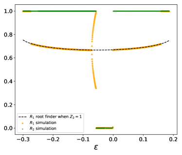
Figure 3: Bifurcation diagram illustrating the stability of the chimera states of the two coupled maps of the mean fields (42). Scatter plots depict the stable solutions (after transient) obtained from the direct simulation of the coupled maps (42), showing $|Z_{1}|$ (orange) and $|Z_{2}|$ (green). The dashed line is the fixed point of the coupled map dynamics found via numerical solver (the findroot function of the mpmath package Johansson et al. (2013)) while assuming one of the mean fields is 1 (at full synchrony).

Here we consider a setup similar to the one studied in Ref. Martens et al. (2016), where two populations of identical continuous-time oscillators interact, with each population more strongly coupled within itself than to the other population. To formulate the corresponding Möbius map model, we denote coupled phases in the two populations by their complex exponentials as before, $z_{1,j}=\exp(i\varphi_{1,j})$ and $z_{2,j}=\exp(i\varphi_{2,j})$, and the corresponding mean field of each population as

$$Z_{1}=\frac{1}{N_{1}}\sum_{j=1}^{N_{1}}z_{1,j}~{},\quad Z_{2}=\frac{1}{N_{2}}\sum_{j=1}^{N_{2}}z_{2,j}\;.$$

The forces acting on the populations are linear combinations of these mean fields

$$Y_{1}e^{i\Psi_{1}} =pZ_{1}+(1-p)Z_{2}\;,$$ (40)

$$Y_{2}e^{i\Psi_{2}} =pZ_{2}+(1-p)Z_{1}\;,$$

where parameter $p$ defines relative strengths of intra- and inter-population couplings. The resulting Möbius maps for the phase variables are

$$z^{(n+1)}_{1,j} =\frac{z^{(n)}_{1,j}+e^{i(\Psi_{1}^{(n)}-\alpha)}\tanh(\frac{\varepsilon Y_{1}}{2})}{1+z^{(n)}_{1,j}e^{-i(\Psi_{1}^{(n)}-\alpha)}\tanh(\frac{\varepsilon Y_{1}}{2})}~{},$$ (41)

$$z^{(n+1)}_{2,j} =\frac{z^{(n)}_{2,j}+e^{i(\Psi_{2}^{(n)}-\alpha)}\tanh(\frac{\varepsilon Y_{2}}{2})}{1+z^{(n)}_{2,j}e^{-i(\Psi_{2}^{(n)}-\alpha)}\tanh(\frac{\varepsilon Y_{2}}{2})}~{},$$

where $\alpha$ is the common phase shift and $\varepsilon$ is the common coupling strength. Here we set the identical frequency to zero by going into a co-rotating frame with the common natural frequency.

In the thermodynamical limit, i.e., $N_{1},N_{2}\rightarrow\infty$, assuming that both systems are on the OA manifold, we can write the dynamics of the coupled system as two coupled maps of the order parameters $Z_{1,2}$ (according to Eq. (16))

$$Z^{(n+1)}_{1} =\frac{Z_{1}^{(n)}+e^{i(\Psi_{1}-\alpha)}\Gamma_{1}}{1+Z_{1}^{(n)}e^{-i(\Psi_{1}-\alpha)}\Gamma_{1}}~{},$$ (42)

$$Z^{(n+1)}_{2} =\frac{Z_{2}^{(n)}+e^{i(\Psi_{2}-\alpha)}\Gamma_{2}}{1+Z_{2}^{(n)}e^{-i(\Psi_{2}-\alpha)}\Gamma_{2}}~{},$$

where $\Gamma_{1}=\tanh(\varepsilon Y_{1}/2)$, $\Gamma_{2}=\tanh(\varepsilon Y_{2}/2)$. $Y_{1,2}$ and $\Psi_{1,2}$ expressed by Eq. (40). For small values of coupling strength $\varepsilon$ these equations integrate the continuous-time attractively or repulsively coupled system. Effects unique to the map model can be expected for large values of $\varepsilon$.

A bifurcation diagram of the mean-field dynamics (42) is shown in Fig. 3. For the numerical simulations, as in Ref. Martens et al. (2016), we choose $\alpha=0.5\pi-0.025$, in-group coupling ratio $p=0.6$, and start iterations at initial order parameters $Z_{1,2}^{(0)}$ with small initial amplitudes, either close to in-phase or to anti-phase. We first evolve the coupled maps (42) according to various positive coupling strength $\varepsilon$. At low coupling strength, depending on the initial conditions $Z_{1,2}^{(0)}$, we obtain either complete synchronization or chimera states, where one of the population is in full synchrony and the other in partial synchrony. At high coupling strength, both populations are in globally stable full synchrony.

For negative $\varepsilon$, we see four regimes. At $\varepsilon_{cr}^{-}<\varepsilon$, corresponding to desynchronization by repulsive coupling in the continuous-time phase model, we observe only the complete asynchronous case with vanishing order parameter. As we decrease $\varepsilon$ further, we see first a period-two chimera, then a chimera with stationary amplitudes, followed by a coexistence of complete synchronization and chimera, and finally complete synchronization of both populations. This can be contrasted again with continuous-time dynamics, where under negative coupling both order parameters can only decrease to zero.

Stable amplitude chimera states are found by numeric evolution of (42) and continued by root finding algorithm into unstable parameter regions. When we increase the negative coupling strength to values larger than $\varepsilon\approx-0.07$, a period-doubling bifurcation of the chimera amplitude occurs, corresponding to a periodic or quasi-periodic mean field. As $\varepsilon$ continues to increase to about $-0.06$ the quasi-periodic orbit collides with full synchronization and both disappear. The asynchronous state becomes stable. The loss of stability of the chimera state for a large positive coupling strength at $\varepsilon\approx 0.16$, similar to a large negative coupling, is again an effect of the discrete map dynamics.

IV.3 Chimera on a ring

Figure 4: Chimera states on a ring in the model described by Eqs. (43) and (44). Panel (a): configuration of the phases; panel (b): the local field amplitude. The chimera pattern shown here appears stable after 18000 steps. The network size is $N=256$, coupling strength $\varepsilon=-0.8$, kernel function parameter $B=0.995$ and phase lag $\alpha=\pi/2-0.18$. Same as the initial condition in Ref. Abrams and Strogatz (2004) for the continuous dynamics, we use $\varphi(t=0)=6r\exp(-0.76x^{2})$, where $r\in[-1/2,1/2]$ is randomly sampled.

The first example of a chimera state for continuous-time oscillators was on a one-dimensional ring with non-local coupling, which was explored by Kuramoto and Battogtokh Kuramoto and Battogtokh (2002); Abrams and Strogatz (2004). The oscillators are coupled via a kernel function, which determines the spatial extent of the interactions with their neighbors. We can show similar chimera states under the coupled Möbius map model as follows.

The oscillators on the ring have positions $x_{j}=2\pi j/N$, where $N$ is the total number. Following Ref. Abrams and Strogatz (2004), we have chosen the coupling kernel as $g_{jm}=1+B\cos(x_{j}-x_{m})$, so that the complex field acting on oscillator $j$ is calculated as

$$U_{j}=R_{j}e^{i\Theta_{j}}=\frac{1}{N}\sum\limits^{N}_{m=1}g_{jm}e^{i\varphi_{m}}~{}.$$ (43)

The phases are driven by these local fields according to the Möbius map

$$z^{(n+1)}_{j}=\frac{z^{(n)}_{j}+e^{i(\Theta_{j}^{(n)}-\alpha)}\tanh(\frac{\varepsilon R_{j}^{(n)}}{2})}{1+z^{(n)}_{j}e^{-i(\Theta_{j}^{(n)}-\alpha)}\tanh(\frac{\varepsilon R_{j}^{(n)}}{2})}~{},$$ (44)

where, as before, $z_{j}=\exp(i\varphi_{j})$.

Similar to the continuous dynamics in Ref. Abrams and Strogatz (2004), we can obtain a stable chimera pattern for a range of positive values of $\varepsilon$ (e.g. $\varepsilon=0.025$) (not shown). Same as in the two-population case before, under discrete map dynamics, there exists a regime under large negative coupling strength which can give rise to a stable chimera pattern, see for example Fig. 4.

Besides the cosine kernel function, we have also simulated the case with a square kernel, i.e., with the local field

$$U_{j}=\frac{1}{2L+1}\sum\limits^{m=L}_{m=-L}\exp[i\varphi_{m+j}]~{}.$$ (45)

Iterating map (44) using this new local field with $N=1000$, $L=130$, $\varepsilon=0.025$ and $\alpha=2.71$, we obtained a many-headed chimera state as in the continuous case in Ref. Maistrenko et al. (2014).

V Conclusion

In this paper we propose a method of modelling synchronizing phase dynamics using a Möbius map. This map reproduces the dynamics of continuous-time phase oscillators. It can be an ideal choice for fast simulation of phase synchronization, since it inherits all the properties of continuous-time phase dynamics. In particular, neither clustering nor chaos under the iteration of a sequence of Möbius maps can occur. All continuous-time models based on the Adler equation, i.e. with a frequency bias and forcing proportional to the first phase harmonics, can be equivalently studied via Möbius maps. We mention here, that also phase coupling models with pure higher-harmonics couplings Gong and Pikovsky (2019) can be modelled with correspondingly modified Möbius maps.

With the proposed Möbius map, we have studied map analogues of known continuous-time models for oscillator ensembles with various connection topologies: the globally coupled Kuramoto-Sakaguchi model, two coupled populations of identical oscillators, and identical oscillators on a ring with non-local coupling via cosine or square distance kernel. For small coupling strengths and small free rotation time step, the coupled maps reproduce the dynamics of their continuous-time dynamical counterparts. Especially, we have reproduced known chimera states with the coupled maps under non-local couplings. For large coupling strength, and in particular for large repulsive coupling, the discrete time dynamics can lead to new synchronization phenomena with continuous and discontinuous bifurcations to synchrony. This phenomenon is not observed in the equivalent continuous-time models.

Appendix A Möbius group property

The Möbius group property implies that the composition of Möbius maps is again a Möbius map. It can be shown as follows:

$$\mathcal{M}_{q_{2},\psi_{2}} = \mathcal{M}_{q_{1},\psi_{1}}\circ\mathcal{M}_{q_{0},\psi_{0}}$$ (46)

$$= \frac{q_{1}+e^{i\psi_{1}}\frac{q_{0}+e^{i\psi_{0}}z}{1+q_{0}^{*}e^{i\psi_{0}}z}}{1+q_{1}^{*}e^{i\psi_{1}}\frac{q_{0}+e^{i\psi_{0}}z}{1+q_{0}^{*}e^{i\psi_{0}}z}}$$

$$= \frac{q_{1}+q_{1}q_{0}^{*}e^{i\psi_{0}}z+q_{0}e^{i\psi_{1}}+e^{i\psi_{0}}e^{i\psi_{1}}z}{1+q_{0}^{*}e^{i\psi_{0}}z+q_{1}^{*}q_{0}e^{i\psi_{1}}+q_{1}^{*}e^{i\psi_{1}}e^{i\psi_{0}}z}$$

$$= \frac{\frac{q_{1}+e^{i\psi_{1}}q_{0}}{1+q_{1}^{*}e^{i\psi_{1}}q_{0}}+\frac{q_{1}q_{0}^{*}+e^{i\psi_{1}}}{1+q_{1}^{*}q_{0}e^{i\psi_{1}}}e^{i\psi_{0}}z}{1+\frac{q_{0}^{*}+q_{1}^{*}e^{i\psi_{1}}}{1+q_{1}^{*}q_{0}e^{i\psi_{1}}}e^{i\psi_{0}}z}$$

$$= \frac{\frac{q_{1}+e^{i\psi_{1}}q_{0}}{1+q_{1}^{*}e^{i\psi_{1}}q_{0}}+\frac{q_{1}q_{0}^{*}+e^{i\psi_{1}}}{1+q_{1}^{*}q_{0}e^{i\psi_{1}}}e^{i\psi_{0}}z}{1+\frac{q_{1}q_{0}^{*}+e^{i\psi_{1}}}{q_{1}q_{0}^{*}+e^{i\psi_{1}}}\frac{q_{0}^{*}+q_{1}^{*}e^{i\psi_{1}}}{1+q_{1}^{*}q_{0}e^{i\psi_{1}}}e^{i\psi_{0}}z}$$

$$= \frac{\frac{q_{1}+e^{i\psi_{1}}q_{0}}{1+q_{1}^{*}e^{i\psi_{1}}q_{0}}+\frac{q_{1}q_{0}^{*}+e^{i\psi_{1}}}{1+q_{1}^{*}q_{0}e^{i\psi_{1}}}e^{i\psi_{0}}z}{1+\frac{q_{1}^{*}+e^{-i\psi_{1}}q_{0}^{*}}{1+q_{1}e^{-i\psi_{1}}q_{0}^{*}}\frac{q_{1}q_{0}^{*}+e^{i\psi_{1}}}{1+q_{1}^{*}q_{0}e^{i\psi_{1}}}e^{i\psi_{0}}z}$$

$$= \frac{\mathcal{M}_{q_{1},\psi_{1}}(q_{0})+\mathcal{C}_{q_{1}q_{0}^{*}}(e^{i\psi_{1}})e^{i\psi_{0}}z}{1+\mathcal{M}^{*}_{q_{1},\psi_{1}}(q_{0})\mathcal{C}_{q_{1}q_{0}^{*}}(e^{i\psi_{1}})e^{i\psi_{0}}z}$$

$$= \frac{q_{2}+e^{i\psi_{2}}z}{1+q_{2}^{*}e^{i\psi_{2}}z}~{}.$$

A direct comparison of the last two expressions in (46) gives rise to the transformation rules Eqs. (8) for the group parameters

$$q_{2}=\mathcal{M}_{q_{1},\psi_{1}}(q_{0}),\quad e^{i\psi_{2}}=\mathcal{C}_{q_{1}q_{0}^{*}}(e^{i\psi_{1}})e^{i\psi_{0}}~{}.$$ (47)

Appendix B Dynamics of the Möbius map

To find the fixed points of the discrete iterated map dynamics  (9) with constant map parameters $q$ and $\psi$, we solve the corresponding quadratic equation

$$z^{2}-\frac{e^{i\psi}-1}{q^{*}e^{i\psi}}z-\frac{q}{q^{*}e^{i\psi}}=0\;.$$ (48)

Eq. (48) has two solutions $z_{1}$ and $z_{2}$ with the properties

$$z_{1}z_{2}=-\frac{q}{q^{*}}e^{-i\psi}\;,\quad z_{1}+z_{2}=\frac{e^{i\psi}-1}{q^{*}e^{i\psi}}\;.$$ (49)

From the first property it follows that $|z_{1}||z_{2}|=1$, which implies that either the two fixed points are on the unit circle, or that one fixed point is inside and the other outside the unit circle. According to this observation, we make the general ansatz

$$z_{1}=\kappa e^{i(\xi+\Delta)}\;,\qquad z_{2}=\frac{1}{\kappa}e^{i\left(\xi-\Delta\right)}\;.$$ (50)

Denoting $q=\rho\cdot\exp(i\vartheta)$ with $0\leq\rho<1$, we obtain from (49) the following two relations:

$$\xi = \vartheta-\frac{\psi-\pi}{2}~{},$$ (51)

$$\sin\frac{\psi}{2} = \frac{\rho}{2}\left[\left(\kappa+\frac{1}{\kappa}\right)\cos\Delta+i\left(\kappa-\frac{1}{\kappa}\right)\sin\Delta\right].\qquad$$ (52)

The two fixed points do not uniquely determine the Möbius group parameters $q$ and $\psi$. In the first regime, the two fixed points are on the unit circle, which implies $\kappa=1$. As a result, the second relation (52) is simplified to

$$\rho\cos\Delta=\sin\frac{\psi}{2}~{}.$$ (53)

The condition for fixed points on the unit circle is therefore

$$\rho>\left|\sin\frac{\psi}{2}\right|~{}.$$ (54)

One of the fixed points is stable and the other unstable, so under this condition the dynamics of the single iterated Möbius map is trivial, and the rotation number is $0$. When equality holds in Eq. (54), it corresponds to the tangent bifurcation point, where the two fixed points merge into one.

In the second regime, $\kappa<1$, i.e., $z_{1}$ is inside the unit circle, then Eq. (52) yields two results

$$\Delta = 0$$ (55)

$$\kappa = \rho^{-1}\left(\sin\frac{\psi}{2}\pm\sqrt{\sin^{2}\frac{\psi}{2}-\rho^{2}}\right)~{}.$$ (56)

For $\kappa$ to be a real number, $\rho\leq|\sin(\psi/2)|$ must be satisfied, which is the exact opposite condition from Eq. (54). Under this set of map parameters, i.e., $\rho\leq|\sin(\psi/2)|$, map  (9) shows rotational dynamics, which can be reduced to a pure rotation by virtue of a transformation which is also a Möbius map

$$y^{(n)}=\mathcal{C}_{-z_{1}}\left(z^{(n)}\right)$$ (57)

The resulting pure rotational dynamics is

$$y^{(n+1)}=\mathcal{C}_{-z_{1}}\circ\mathcal{M}_{q,\psi}\circ\mathcal{C}_{z_{1}}\left(y^{(n)}\right)=\mathcal{R}_{2\pi\eta}\left(y^{(n)}\right)~{},$$ (58)

with the fixed point $z_{1}=\kappa\cdot\exp(i\xi)$ as the group parameter, and the rotation number is

$$\eta=\frac{1}{\pi}\arctan\left(\tan\frac{\psi}{2}\cdot\sqrt{1-\frac{\rho^{2}}{\sin^{2}\frac{\psi}{2}}}\right)~{}.$$ (59)

Eq. (59) shows that in this second regime, the rotation number $\eta$ is a smooth function of the map parameters $\psi$ and $\rho$.

Appendix C Ott-Antonsen manifold for an ensemble of Möbius maps

The transformation $\mu_{Q,\Psi}$ of a uniform phase density $\mu_{0}(\varphi)=1/(2\pi)$ under Möbius transformation $\exp(i\varphi)\to\mathcal{M}_{Q,\Psi}(\exp(i\varphi))$ of the unit circle is a wrapped Cauchy distribution

$$\mu_{Q,\Psi}(\varphi)=\mu_{Q}(\varphi)=\frac{1}{2\pi}\frac{1-|Q|^{2}}{|e^{i\varphi}-Q|^{2}}~{},$$ (60)

also known as the (univariate) Poisson kernel Marvel et al. (2009). To show (60) is true, we can calculate the characteristic function, which are just the circular moments $\left\langle\exp(ik\varphi)\right\rangle_{\mu_{Q,\Psi}}$ of the distribution $\mu_{Q,\Psi}$, and compare that to the characteristic function of the Poisson kernel. For the circular moments of phases with density $\mu_{Q,\Psi}$, we have

$$\left\langle e^{ik\varphi}\right\rangle_{\mu_{Q,\Psi}} = \int_{0}^{2\pi}e^{ik\varphi}\mu_{Q,\Psi}(\varphi)d\varphi$$

$$= \int_{0}^{2\pi}\left(\mathcal{M}_{Q,\Psi}\left(e^{i\varphi}\right)\right)^{k}\mu_{0}(\varphi)d\varphi$$

$$= \frac{1}{2\pi}\int_{0}^{2\pi}\left(\frac{Q+e^{i(\Psi+\varphi)}}{1+Q^{*}e^{i(\Psi+\varphi)}}\right)^{k}d\varphi$$

$$= \frac{1}{2\pi i}\oint_{|z|=1}\frac{1}{z}\left(\frac{Q+z}{1-Q^{*}z}\right)^{k}dz=Q^{k}~{},$$

where the last integral after the substitution $d\varphi=dz/(iz)$ is a complex contour integral with a simple pole $z=0$ inside and a $k$th-order pole $z=(Q^{*})^{-1}$ outside of the unit circle. In the derivation above we have also used the fact that the integral over the unit circle with respect to the transformed density $\mu_{Q,\Psi}$ is equal to the integral of the transformed circle $\mathcal{M}_{Q,\Psi}\left(S^{1}\right)$ with respect to the uniform density $\mu_{0}$.

From (C), first, we see that indeed the characteristic function, and therefore the distribution $\mu_{Q,\Psi}=\mu_{Q}$ is independent of $\Psi$. Second, the circular moments are integer powers of the Möbius map parameter $Q$, and in particular, the first moment $Z=\left\langle\exp(i\varphi)\right\rangle_{\mu_{Q}}=Q$.

The circular moments of the Poisson kernel can be similarly obtained via complex integration. Given $z=\exp(i\varphi)$ and $d\varphi=dz/(iz)$, it follows

$$\left\langle e^{ik\varphi}\right\rangle = \frac{1}{2\pi}\int_{0}^{2\pi}e^{ik\varphi}\frac{1-|Q|^{2}}{|e^{i\varphi}-Q|^{2}}d\varphi$$

$$= \frac{1}{2\pi}\int_{0}^{2\pi}\frac{e^{i(k+1)\varphi}(1-|Q|^{2})}{(e^{i\varphi}-Q)(1-Q^{*}e^{i\varphi})}d\varphi$$

$$= \frac{1}{2\pi i}\oint_{|z|=1}\frac{z^{k}(1-|Q|^{2})}{1-Q^{*}z}\frac{1}{(z-Q)}dz=Q^{k}~{}.$$

Since they have the same characteristic function, the density function $\mu_{Q}$ must be identical to the Poisson kernel, i.e. Eq. 60.

Appendix D Solution of Adler equation over a finite time interval

Here we will show that the kick map

$$\mathcal{K}_{\lambda,A\tau,\beta}\left(z\right)=\frac{(\sigma+i\lambda\Gamma)z+e^{i\beta}\Gamma}{(\sigma-i\lambda\Gamma)+ze^{-i\beta}\Gamma}$$ (63)

with $\sigma=\sqrt{1-\lambda^{2}}$ and $\Gamma=\tanh(A\tau\sigma/2)$ under the conventions $\sqrt{-1}=i$ and $\tanh(ix)=i\tan(x)$ is indeed a solution of the Adler equation

$$\dot{\varphi}=A\left[\lambda-\sin(\varphi-\beta)\right]$$ (64)

with constant parameters $A$, $\lambda$ and $\beta$. With $z=e^{i\varphi}$, (64) can be written in a complex form

$$\dot{z}=izA\left(\frac{1}{2i}e^{i\beta}z^{*}+\lambda-\frac{1}{2i}e^{-i\beta}z\right)~{}.$$ (65)

The parameters of the kick map can be directly taken from the Adler equation, and the kick map can be easily cast into the canonical form (1) of the Möbius map, where

$$q=e^{i\beta}\frac{\Gamma}{\sigma-i\lambda\Gamma}~{},\qquad e^{i\psi}=\frac{\sigma+i\lambda\Gamma}{\sigma-i\lambda\Gamma}~{}.$$ (66)

Note that $\sigma$ and $\Gamma$ are either both real or both imaginary. The complex conjugates of $q$ and $\exp(i\psi)$ are therefore obtained by just replacing $i\to-i$ in the formulas above. Without loss of generality we can make a substitution $z\to z\exp(i\beta)$, $q\to q\exp(i\beta)$ and consider only $\beta=0$. Marvel et al. Marvel et al. (2009) have shown that for phase equations (65), with arbitrary time dependence of the parameters, the solution is given by a Möbius transform where the parameters evolve according to the ordinary differential equations

$$\dot{q} = A\left(\frac{1}{2}+i\lambda q-\frac{1}{2}q^{2}\right)$$ (67)

$$\dot{\psi} = A\left(\frac{1}{2i}q^{*}+\lambda-\frac{1}{2i}q\right)~{}.$$ (68)

Thus, we just need to show that the same is true for the parameters $q$ and $\psi$ and for our choice of $\Gamma(\tau)$.

The left-hand-side of (67) can be calculated as

$$\dot{q}=\frac{\sigma\dot{\Gamma}}{(\sigma-i\lambda\Gamma)^{2}}=\frac{\sigma^{2}\frac{A}{2}(1-\Gamma^{2})}{(\sigma-i\lambda\Gamma)^{2}}~{},$$ (69)

which matches the right-hand-side

$$A\left(\frac{1}{2}+i\lambda q-\frac{1}{2}q^{2}\right)$$

$$= \frac{A}{(\sigma-i\lambda\Gamma)^{2}}\left(\frac{1}{2}(\sigma-i\lambda\Gamma)^{2}+i\lambda\Gamma(\sigma-i\lambda\Gamma)-\frac{1}{2}\Gamma^{2}\right)$$

$$= \frac{A}{(\sigma-i\lambda\Gamma)^{2}}\left(\frac{1}{2}\sigma^{2}+\frac{1}{2}\lambda^{2}\Gamma^{2}-\frac{1}{2}\Gamma^{2}\right)$$

$$= \frac{\frac{A}{2}}{(\sigma-i\lambda\Gamma)^{2}}\left(\sigma^{2}-(1-\lambda^{2})\Gamma^{2}\right)=\frac{\sigma^{2}\frac{A}{2}(1-\Gamma^{2})}{(\sigma-i\lambda\Gamma)^{2}}~{}.$$

This proves the first identity (67). Similarly, we observe

$$\frac{d}{d\tau}e^{i\psi}=\frac{2i\lambda\sigma\dot{\Gamma}}{(\sigma-i\lambda\Gamma^{2})}=i\lambda Ae^{i\psi}\frac{\sigma^{2}(1-\Gamma^{2})}{\sigma^{2}+\lambda^{2}\Gamma^{2}}$$ (71)

and

$$ie^{i\psi}A\left(\frac{1}{2i}q^{*}+\lambda-\frac{1}{2i}q\right)$$

$$= iAe^{i\psi}\left(\frac{1}{2i}\frac{\Gamma}{\sigma+i\lambda\Gamma}+\lambda-\frac{1}{2i}\frac{\Gamma}{\sigma-i\lambda\Gamma}\right)$$

$$= iAe^{i\psi}\frac{\frac{1}{2}\Gamma(\sigma-i\lambda\Gamma)+i\lambda(\sigma^{2}+\lambda^{2}\Gamma^{2})-\frac{1}{2}\Gamma(\sigma+i\lambda\Gamma)}{i(\sigma^{2}+\lambda^{2}\Gamma^{2})}$$

$$= iAe^{i\psi}\frac{\lambda(\sigma^{2}+\lambda^{2}\Gamma^{2})-\lambda\Gamma^{2}}{\sigma^{2}+\lambda^{2}\Gamma^{2}}=i\lambda Ae^{i\psi}\frac{\sigma^{2}(1-\Gamma^{2})}{\sigma^{2}+\lambda^{2}\Gamma^{2}}~{},$$

which proves the second identity (68).

Unlike those of the standard parametrization of the Möbius map (1) (Appendix (B)), the fixed points of the kick map (63) have a more direct relation to the parameters. The fixed point equation

$$z=\frac{(\sigma+i\lambda\Gamma)z+\Gamma}{(\sigma-i\lambda\Gamma)+z\Gamma}$$ (73)

can be changed into the quadratic form $z^{2}-1-2i\lambda z=0$ which is solved by

$$z=i\lambda\pm\sqrt{1-\lambda^{2}}=i\lambda\pm\sigma~{}.$$ (74)

If $|\lambda|<1$, the fixed points of the kick map are located on the unit circle at phases $\varphi$ with $\sin\varphi=\lambda$ and $\cos\varphi=\pm\sigma$. If $|\lambda|>1$, the fixed points are on the imaginary axis inside and outside the unit circle at $i(\lambda\pm\sqrt{\lambda^{2}-1})$. In both cases the locations of the fixed points are independent of $\Gamma$, i.e. of the kick map parameter $A\tau$, which only controls the degree of contraction, expansion or rotation around the fixed points and not their locations.

Appendix E Computational efficiency of Möbius map models

For a single iterated map, due to the complexity inherent in the algebraic form of the map, a single step with the Möbius map Eq. (18) is 2.5 times slower than the sine map, or equivalently, than an Euler integration step of the corresponding ODE system (21). However, when integrating Adler equation, whose property is inherited by the equivalent Möbius map, the time step $\tau$ can be large and a significant speed-up can be achieved.

Nevertheless, for systems of globally or locally coupled oscillators, the main bottleneck in terms of computational efficiency is the calculation of the mean fields. This bottleneck remains also under the application of Möbius maps. Euler integration and Möbius map each requires one calculation of the mean field in every step which takes about the same time. This is confirmed by double precision Euler integration of the Kuramoto-Sakaguchi Model Eq. (27), as compared to simulations with Möbius map model Eq. (29). When Runge-Kutta integration is used, which requires four evaluations of the mean field per integration step, the method using Möbius map is four times faster, similar to Euler scheme.

However, while Euler scheme violates partial integrability of the original globally coupled ODE dynamics, Möbius map preserves such property Gong et al. (2019). Certainly, many synchronization effects can also be observed in the integrations of ODEs with large integration steps, even with correspondingly large integration errors. The main distinction of Möbius map from the integration of ODEs is the invariance of the OA manifold. When a more precise solution of the ODE system is required, the time step usually needs to decrease by a factor of 10 or 100, which makes integrating ODE correspondingly much slower compared to evolving the system using Möbius maps.

In fact, using Watanabe-Strogatz theory, we can combine Möbius maps with a numerical integration of the reduced quasi-mean-field equations, i.e. ODEs (67) and (68), for the Möbius group parameters to obtain ODE solutions of the full system to desired precision that conserve all constants of motion (see Ref. Marvel et al. (2009) and a practical example in Ref. Gong and Pikovsky (2019)) but the necessary calculation of the mean field from the constants of motion is computationally more involved than an integration with regular numerical schemes, because an additional transformation from the constants to the phases is needed at every integration step.

References

- Kuramoto (1975) Y. Kuramoto, in International Symposium on Mathematical Problems in Theoretical Physics, Lecture Notes in Physics, Vol. 39 (Springer, New York, NY, USA, 1975), pp. 420–422.
- Pazó and Montbrió (2014) D. Pazó and E. Montbrió, Physical Review X 4, 011009 (2014).
- Cabral et al. (2011) J. Cabral, E. Hugues, O. Sporns, and G. Deco, NeuroImage 57, 130 (2011), ISSN 1053-8119.
- Petkoski et al. (2018) S. Petkoski, J. M. Palva, and V. K. Jirsa, PLOS Computational Biology 14, 1 (2018).
- Breakspear et al. (2010) M. Breakspear, S. Heitmann, and A. Daffertshofer, Frontiers in Human Neuroscience 4, 190 (2010).
- Montbrió and Pazó (2018) E. Montbrió and D. Pazó, Phys. Rev. Lett. 120, 244101 (2018).
- Doesburg et al. (2009) S. M. Doesburg, J. J. Green, J. J. McDonald, and L. M. Ward, PLOS ONE 4, 1 (2009).
- Malagarriga et al. (2015) D. Malagarriga, M. García-Vellisca, A. E. Villa, J. Buldú, J. García-Ojalvo, and A. Pons, Frontiers in Computational Neuroscience 9, 97 (2015), ISSN 1662-5188.
- Soman et al. (2018) K. Soman, V. Muralidharan, and V. S. Chakravarthy, Frontiers in Computational Neuroscience 12, 52 (2018), ISSN 1662-5188.
- Hoppensteadt and Izhikevich (2000) F. C. Hoppensteadt and E. M. Izhikevich, IEEE Transactions on Neural Networks 11, 734 (2000).
- Chakraborty et al. (2014) S. Chakraborty, J. Dalal, B. Sarkar, and D. Mukherjee, 2014 International Conference on Signal Propagation and Computer Technology (ICSPCT 2014) pp. 368–375 (2014).
- Vodenicarevic et al. (2016) D. Vodenicarevic, N. Locatelli, J. Grollier, and D. Querlioz, in 2016 International Joint Conference on Neural Networks (IJCNN) (2016), pp. 2015–2022.
- Zhang et al. (2019) T. Zhang, M. R. Haider, Y. Massoud, and J. I. D. Alexander, Electronics 8, 64 (2019), ISSN 2079-9292.
- Heger and Krischer (2016) D. Heger and K. Krischer, Phys. Rev. E 94, 022309 (2016).
- Sakaguchi and Kuramoto (1986) H. Sakaguchi and Y. Kuramoto, Progress of Theoretical Physics 76, 576 (1986).
- Winfree (1967) A. T. Winfree, Journal of Theoretical Biology 16, 15 (1967).
- Kaneko (1990) K. Kaneko, Phys. Rev. Lett. 65, 1391 (1990).
- Kaneko (1991) K. Kaneko, Physica D 54, 5 (1991), ISSN 0167-2789.
- Nozawa (1992) H. Nozawa, Chaos: An Interdisciplinary Journal of Nonlinear Science 2, 377 (1992).
- Pikovsky and Kurths (1994) A. S. Pikovsky and J. Kurths, Physica D 76, 411 (1994).
- Just (1995) W. Just, Physica D 81, 317 (1995).
- Topaj et al. (2001) D. Topaj, W.-H. Kye, and A. Pikovsky, Phys. Rev. Lett. 87, 074101 (2001).
- Chatterjee and Gupte (1996) N. Chatterjee and N. Gupte, Phys. Rev. E 53, 4457 (1996).
- Osipov and Kurths (2002) G. Osipov and J. Kurths, Phys. Rev. E 65, 016216 (2002).
- Bauer and Martienssen (2009) M. Bauer and W. Martienssen, Network Computation in Neural Systems 2, 345 (2009).
- Gong et al. (2019) C. C. Gong, C. Zheng, R. Toenjes, and A. Pikovsky, Chaos 29, 033127 (2019).
- Marvel et al. (2009) S. A. Marvel, R. E. Mirollo, and S. H. Strogatz, Chaos 19, 043104. (2009).
- Watanabe and Strogatz (1994) S. Watanabe and S. H. Strogatz, Physica D 74, 197 (1994).
- Pikovsky and Rosenblum (2008) A. S. Pikovsky and M. Rosenblum, Phys. Rev. Lett. 101, 264103 (2008).
- Pikovsky and Rosenblum (2015) A. S. Pikovsky and M. Rosenblum, Chaos 25 (2015).
- Chen et al. (2017) B. Chen, J. R. Engelbrecht, and R. Mirollo, Journal of Physics A 50, 355101 (2017).
- Ott and Antonsen (2008) E. Ott and T. M. Antonsen, Chaos 18, 037113 (2008).
- Griniasty and Hakim (1994) M. Griniasty and V. Hakim, Phys. Rev. E 49, 2661 (1994).
- Abrams et al. (2008) D. M. Abrams, R. Mirollo, S. H. Strogatz, and D. A. Wiley, Phys. Rev. Lett. 101, 084103 (2008).
- Abrams and Strogatz (2004) D. M. Abrams and H. S. Strogatz, Phys. Rev. Lett. 93, 174102 (2004).
- Kuramoto and Battogtokh (2002) Y. Kuramoto and D. Battogtokh, Nonlinear Phenom. Complex Syst. 5, 380 (2002).
- Kalle et al. (2017) P. Kalle, J. Sawicki, A. Zakharova, and E. Schöll, Chaos: An Interdisciplinary Journal of Nonlinear Science 27, 033110 (2017).
- Katok and Hasselblatt (1995) A. Katok and B. Hasselblatt, Introduction to the Modern Theory of Dynamical Systems (Cambridge University Press, 1995).
- Pikovsky et al. (2001) A. S. Pikovsky, M. Rosenblum, and J. Kurths, Synchronization: A Universal Concept in Nonlinear Sciences, Cambridge Nonlinear Science Series (Cambridge University Press, 2001).
- Adler (1946) R. Adler, Proceedings of the IRE 34, 351 (1946), ISSN 0096-8390.
- Buchstaber et al. (2010) V. M. Buchstaber, O. V. Karpov, and S. I. Tertychniy, Theoretical and Mathematical Physics 162, 211 (2010).
- Ilyashenko et al. (2011) Y. S. Ilyashenko, D. A. Ryzhov, and D. A. Filimonov, Functional Analysis and Its Applications 45, 192 (2011).
- Rosenblum and Pikovsky (2004a) M. Rosenblum and A. Pikovsky, Phys. Rev. Lett. 92, 114102 (2004a).
- Rosenblum and Pikovsky (2004b) M. Rosenblum and A. Pikovsky, Phys. Rev. E 70, 041904 (2004b).
- Popovych et al. (2005) O. Popovych, C. Hauptmann, and P. A. Tass, Phys. Rev. Lett. 94, 164102 (2005).
- Popovych et al. (2017) O. V. Popovych, B. Lysyansky, M. Rosenblum, A. Pikovsky, and P. A. Tass, PLOS ONE 12, 1 (2017).
- Johansson et al. (2013) F. Johansson et al., mpmath: a Python library for arbitrary-precision floating-point arithmetic (version 0.18) (2013), http://mpmath.org.
- Martens et al. (2016) E. Martens, M. Panaggio, and D. M. Abrams, New Journal of Physics, Fast Track Communication 18, 022002 (2016).
- Maistrenko et al. (2014) Y. L. Maistrenko, A. Vasylenko, O. Sudakov, R. Levchenko, and V. L. Maistrenko, International Journal of Bifurcation and Chaos 24, 1440014 (2014).
- Gong and Pikovsky (2019) C. C. Gong and A. Pikovsky, Phys. Rev. E 100, 062210 (2019).