Node Masking

Abstract.

Graph Neural Networks (GNNs) have received a lot of interest in the recent times. From the early spectral architectures that could only operate on undirected graphs per a transductive learning paradigm to the current state of the art spatial ones that can apply inductively to arbitrary graphs, GNNs have seen significant contributions from the research community. In this paper, we utilize some theoretical tools to better visualize the operations performed by state of the art spatial GNNs. We analyze the inner workings of these architectures and introduce a simple concept, Node Masking, that allows them to generalize and scale better. To empirically validate the concept, we perform several experiments on some widely-used datasets for node classification in both the transductive and inductive settings, hence laying down strong benchmarks for future research.

1. Introduction

Graphs are the most effective way of representing different types of entities and relationships amongst them. Several constructs inherently involve the notion of graphs, such as social networks, molecular structures, knowledge bases, recommendation systems, etc. Over the past few year, learning on graphs has become increasingly popular, applications of which can be found in domains ranging from detection of abuse online (Mishra et al., 2019) and document classification (Kipf and Welling, 2017) to knowledge graph alignment (Wang et al., 2018) and relation extraction in texts (Sahu et al., 2019). Learning on graphs is essentially about leveraging the inductive bias imposed by their relational structures, i.e., relational inductive bias, so as to achieve better performance on tasks that can benefit from relation reasoning (Battaglia et al., 2018). The ability to exploit relationships amongst entities in the data is a crucial one for advancing the state of artificial intelligence (Tenenbaum et al., 2011; Lake and Baroni, 2017).

A graph is defined by its set of nodes (i.e., vertices) and its set of edges. There exist two different paradigms for learning on graphs, transductive and inductive. In transductive learning, the node and edge sets remain constant across the training and prediction phases. In other words, at the training time, the learning algorithm has access to all the nodes and edges, including those for which predictions are to be made. Note that transductive learning does not support generalization to unseen nodes and edges. Figure 1 depicts node classification performed in a transductive setting.

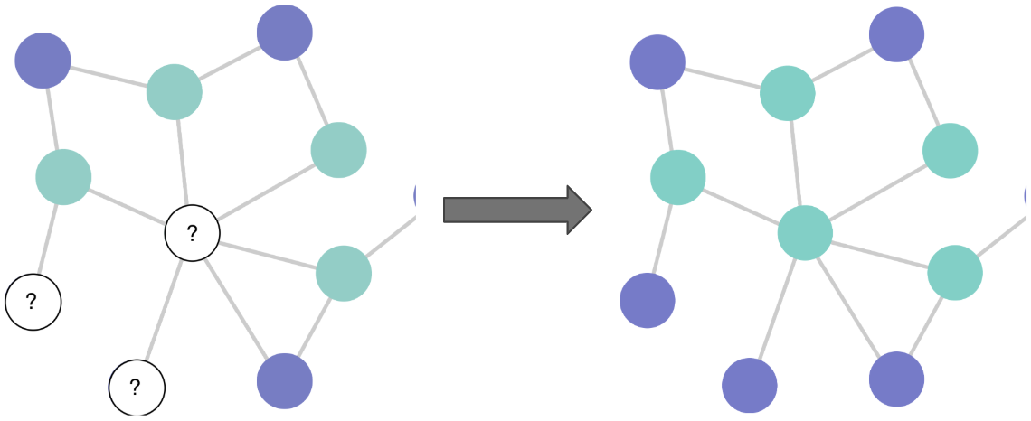
Figure 1. Node classification in transductive settings. At the training time, the learning algorithm has access to all the nodes and edges, including those nodes for which labels are to be predicted (denoted by question marks).

In inductive learning, first a model $\mathcal{H}$ is learned over the training graph consisting of some nodes and edges. The learned model is then used to predict on unseen nodes and edges that may or may not be disconnected from the nodes and edges in the training graph (Chiang et al., 2019). Note that some works (Veličković et al., 2018; Hamilton et al., 2017) have instead interpreted inductive learning to mean that the model is first trained on a set of graphs and then applied to a separate set of graphs. But the former interpretation subsumes the latter in that a set of graphs can be treated as a single graph with multiple disconnected components. Figure 2 depicts node classification in inductive settings.

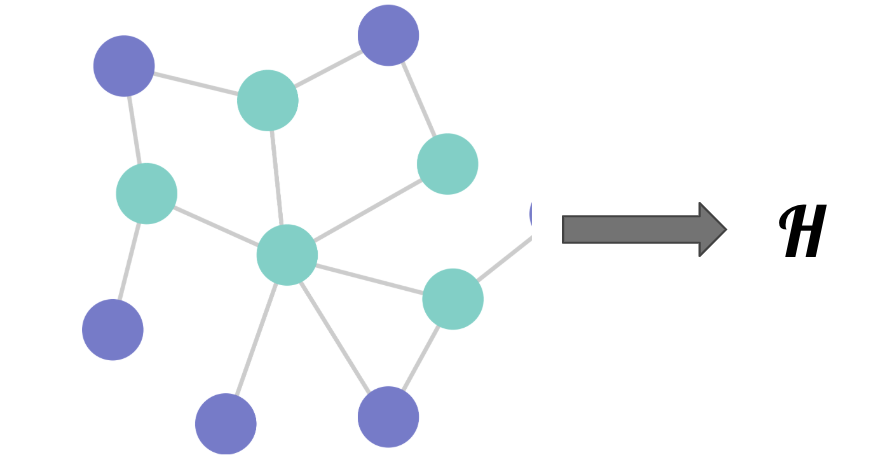
(a) A model $\mathcal{H}$ is learned over some graph

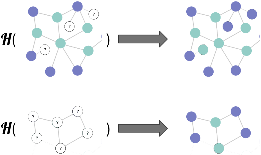
(b) The model is then by applied to new nodes and edges

Figure 2. Node classification in inductive settings. Once learned, the model can be applied to new unseen nodes (denoted by question marks). There may or may not exist edges between such new nodes and the nodes used for training.

Deep learning has brought advancements to several areas within AI. That said, deep learning on graphs is a rather challenging task to perform with traditional architectures like Convolutional Neural Networks or Recurrent Neural Networks. In the recent years, a lot of research has been dedicated to generalizing the convolution operation to graphs (Bruna et al., 2014; Kipf and Welling, 2017; Hamilton et al., 2017; Xu et al., 2019), which has formed the basis of all modern graph neural networks (GNNs). From the early spectral architectures that could only operate on undirected graphs in transductive settings to the current state of the art spatial ones that can apply inductively to arbitrary graphs, GNNs have undergone significant developments. This paper makes contributions towards further enhancing the capabilities of state of the art spatial GNNs.

Our contributions. We first discuss some theoretical tools to better visualize the operations performed by spatial GNNs. Using these tools, we analyze the inner workings of the state of the art spatial architectures, specifically aggregation-based GNNs, to uncover the sources of over-smoothing and over-fitting. We then propose a simple technique called Node Masking to help these GNNs generalize and scale better. We empirically uncover how this technique impacts over-smoothing and over-fitting in GNNs and validate the merits of the technique by performing several experiments on three widely-used benchmark datasets for node classification in both the transductive and inductive settings.

2. A brief history of GNNs

The concept of GNNs was first formalized in the work of Gori et al. (Gori et al., 2005). The authors presented GNNs as an extension of recursive neural networks whereby they treat nodes as objects denoted by state vectors and edges as the relationships amongst those nodes. Their design consists of two main steps: i) iterative update of nodes’ state vectors based on the labels and state vectors of their neighbors up to a stable fixed point, and ii) back-propagation for adjustment of parameters used in the update step. This approach was further refined in the work of Scarselli et al. (Scarselli et al., 2009).

2.1. Spectral GNNs

Bruna et al. (Bruna et al., 2014) laid the foundation for generalization of the convolution operation from regular grids to graphs. Leveraging spectral graph theory, they proposed an architecture for performing spectral convolutions on graphs. Given a graph $G$, their architecture considers the feature vectors on nodes as multi-channel graph signals. It learns spectral filters that act on these signals in the Fourier domain defined by the eigenvectors of the Laplacian matrix of $G$. This architecture displays limited scalability since the filters learned are not localized, i.e., they act on the whole graph, and computation of the Laplacian’s eigenvectors is itself an expensive operation.

To overcome these issues, Defferrard et al. (Defferrard et al., 2016) and Levie et al. (Levie et al., 2017) proposed spectral architectures, ChebNet and CayleyNet respectively, comprising localized filters approximated by Chebyshev and Cayley polynomials. Kipf and Welling (Kipf and Welling, 2017) further simplified ChebNet by making the filters localized to 1-hop neighborhoods. By stacking multiple such filters in layers, they showed that any number of hops could be covered in the convolution operation. They called this new architecture Graph Convolutional Network (GCN). Note that all spectral architectures are inherently transductive in that the filters learned on a graph are specific to the eigenbasis of its Laplacian. This not only limits the ability of these architectures to generalize to new nodes and edges. Although GCN itself is spectral, the idea of stacking multiple layers to cover higher-order neighborhoods led to the concept of spatial GNNs.

2.2. Spatial GNNs

Spatial GNNs define the convolution operation directly on the structure of the graph. In other words, they work by learning functions to compute representations for nodes or edges that capture the features and structures of their surrounding neighborhoods. Once learned, these functions can then be inductively applied to new nodes and edges. Spatial GNNs are preferred over their spectral counterparts due to their scalability, inductive capabilities, and ability to handle myriad types of graphs (Wu et al., 2019).

2.2.1. Sampling-based

GraphSAGE (Hamilton et al., 2017) was one of the first spatial GNNs. For a node $v$, GraphSAGE randomly samples a fixed number of nodes from its $K$-hop neighborhood and learns to computes a representation for $v$ based on its own features plus the features of its sampled neighbors. Note that this design does not exhibit structural invariance, i.e., the GNN cannot accommodate varying neighborhood structures but rather constrains nodes to a fixed number of neighbors only. A clear drawback of such a sampling-based design is that a lot of neighborhood information is wasted.

2.2.2. Aggregation-based

Aggregation-based spatial GNNs eliminate the need for sampling fixed number of neighbors. They work by iteratively computing representations for nodes based on those of their respective neighbors. A $k$-layer aggregation-based GNN sequentially performs such updates $k$ times, consequently computing a representation for every node that captures its $k$-hop neighborhood. The update operation performed by the $k^{th}$ layer for a node $v$ can be stated as:

(1) $$h^{(k)}_{v}=f^{(k)}\,\left(\,h^{(k-1)}_{v},\,g\,(\{h^{(k-1)}_{u}:u\in\mathcal{N}_{v}\})\,\right)$$

where $\mathcal{N}_{v}$ denotes the set of neighbors of $v$, and $h^{(0)}_{v}$ is the input feature vector of $v$. The aggregate function $g$ aggregates representations of neighbors, and the combine function $f$ combines the aggregated representation with that of $v$ itself. This formulation is general enough to cover the various aggregation-based GNNs that exist. All of them mainly differ in their choice of $f$ and $g$. Note that the compute required to capture $k$-hop neighborhood grows linearly with $k$ in aggregation-based GNNs as opposed to exponentially in sampling-based GNNs.

Velickovic et al. (Veličković et al., 2018) proposed Graph Attention Networks (GAT) wherein a node’s representation is iteratively updated by aggregating the representations of its neighbors combining them with that of the node’s as per coefficients allocated by a self-attention mechanism. The defines the update operation in the $k^{th}$ layer as:

(2) $$h^{(k)}_{v}=\bigg{\|}_{l}\,\sigma\left(\,\sum_{u}^{v\,\cup\,\mathcal{N}_{v}}\alpha^{(k)}_{l}(v,u)\cdot W^{(k)}_{l}h^{(k-1)}_{u}\,\right)$$

where $\alpha^{(k)}_{l}(v,u)$ is the attention coefficient of node $u$ with respect to node $v$ from the $l^{th}$ attention head, $W_{l}$ is the weight matrix for the $l^{th}$ attention head, and $\|$ denotes concatenation over the heads.

Xu et al. (Xu et al., 2019) recently introduced the Graph Isomorphism Network (GIN) whose theoretical foundations allows it to be maximally powerful amongst the various spatial GNNs. The GIN-$\epsilon$ architecture defines the update operation as:

(3) $$h^{(k)}_{v}=MLP^{(k)}\left((1+\epsilon^{(k)})\cdot h^{(k-1)}_{v}+\sum_{u}^{\mathcal{N}_{v}}h^{(k-1)}_{u}\right)$$

where $MLP$ represents a multi-layer perceptron.

In this paper, we focus on aggregation-based GNNs given that they yield state of the art (Wu et al., 2019) performance. We work with the GAT and GIN architectures only but our techniques can be applied to other aggregation-based GNNs.

3. Theoretical Framework

Hereon, we assume that the graphs we consider are undirected, implying that an edge can be traversed from either endpoints. That said, the work presented in this paper is trivially applicable to directed graphs too. We also assume that all nodes within a given graph are uniquely identifiable.

3.1. Aggregation trees

We discuss the concept of aggregation trees as the theoretical tool for visualizing aggregation-based GNNs. Aggregation trees have been explored in the past as graph kernels (Xu et al., 2019) under names like tree-walks (Bach, 2008) or subtree patterns (Shervashidze et al., 2011).

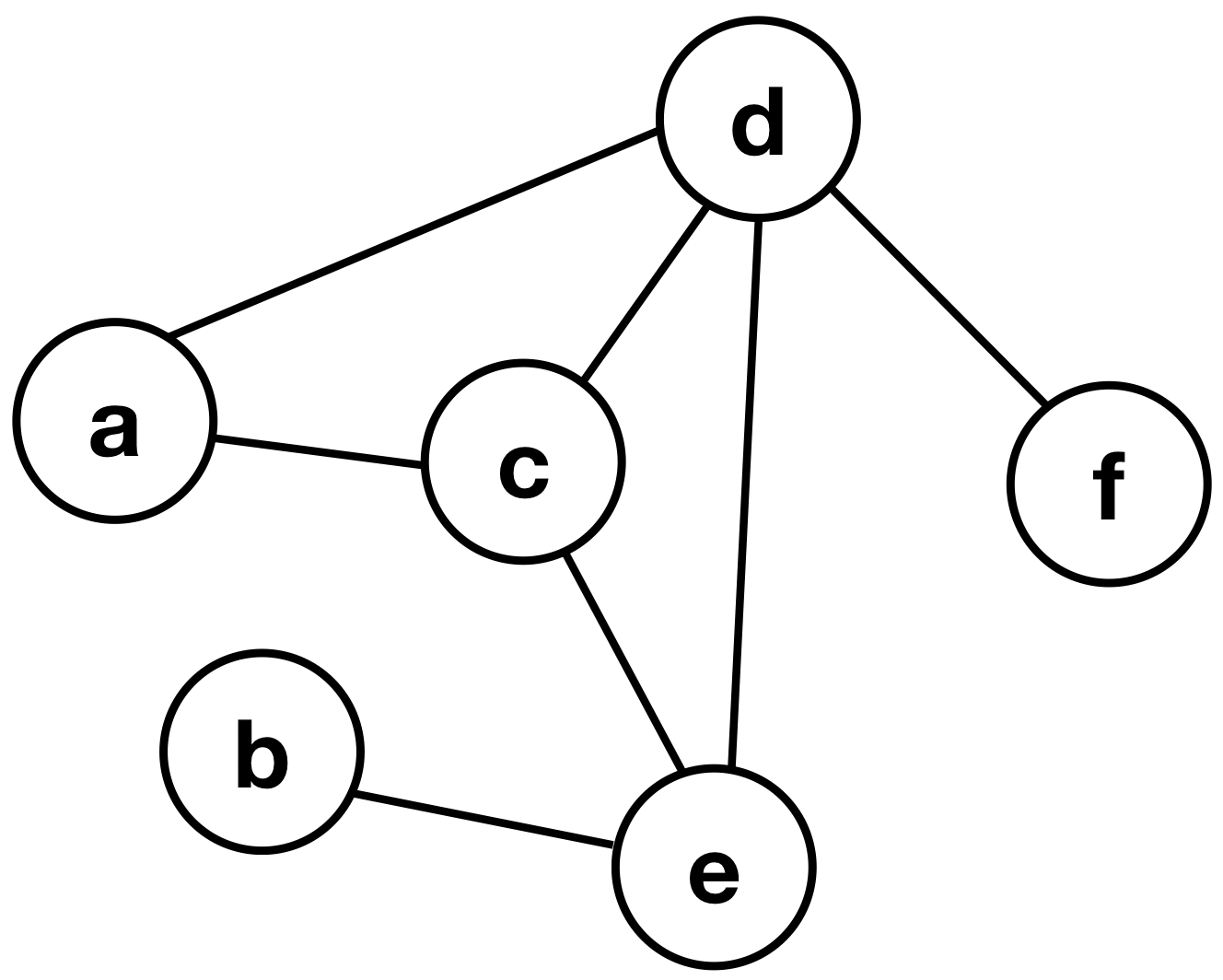
(a) An undirected graph

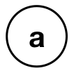
(b) $T_{a}^{0}$

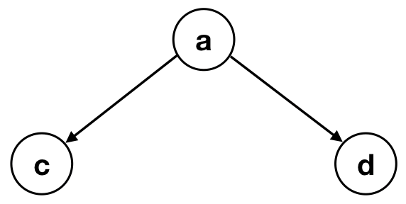
(c) $T_{a}^{1}$

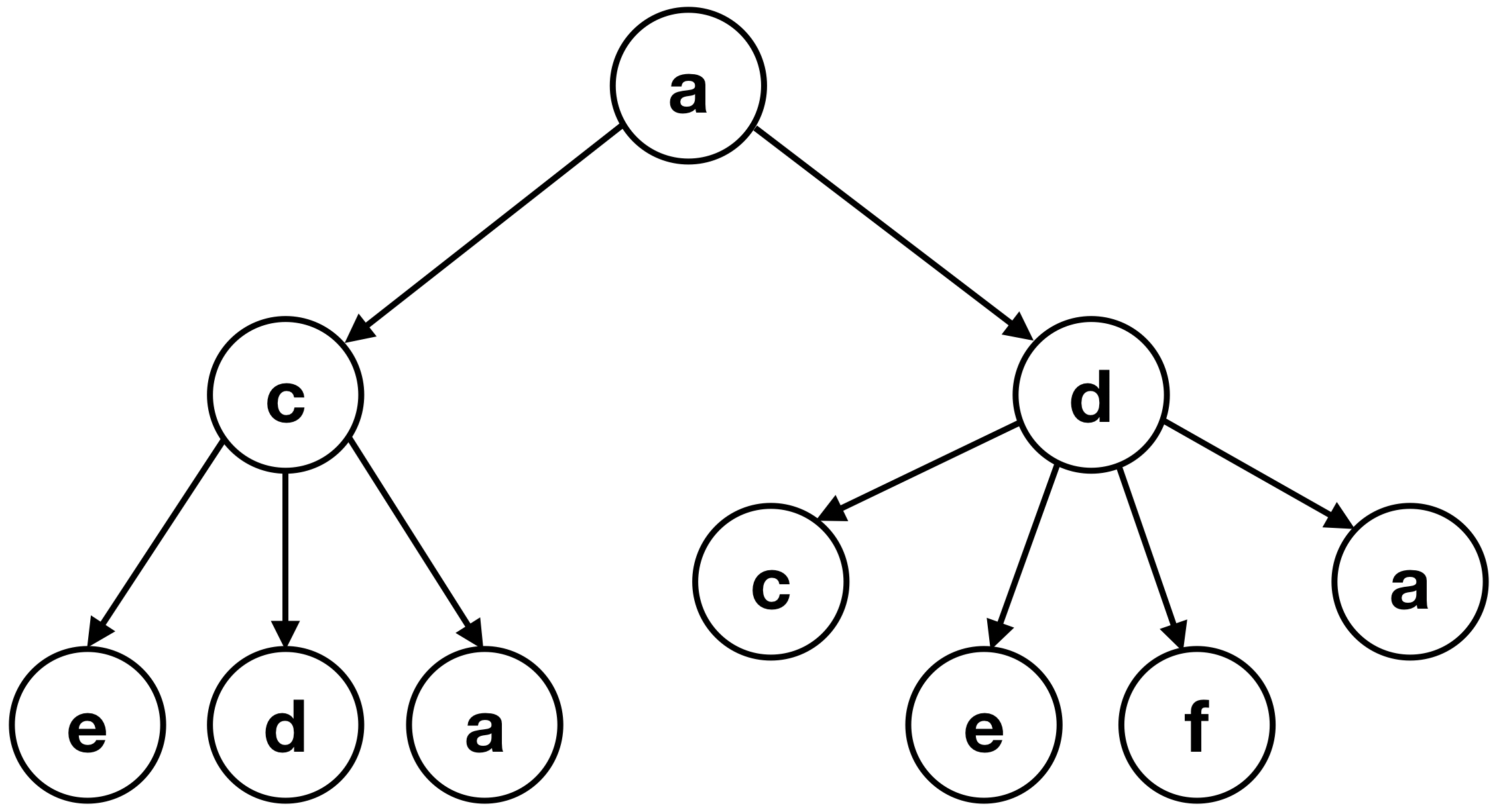
(d) $T_{a}^{2}$

Figure 3. Sub-figure (a) shows an undirected graph, i.e., edges can be walked in either directions. Sub-figures (b-d) show some aggregation trees $T^{k}_{a}$ of node a. Every path from the root of a $T^{k}_{a}$ to some leaf in it is a valid $k$-hop walk in the graph starting at node $a$, and vice versa.

Definition 3.1.

Given a graph $G$ with a node $v$ in it, let $\mathcal{P}_{v}^{k}$ denote the set of all possible walks of length $k$, i.e., of $k$ hops, starting at $v$. Walks are paths with possibly repeated nodes. The $k$-aggregation tree $T_{v}^{k}$ of a node $v$ is the smallest arborescence (Fournier, 2013) rooted at $v$ such that $w$ is a path from the root of $T_{v}^{k}$ to a leaf in it if and only if $w\in\mathcal{P}_{v}^{k}$. Here, smallness is by the number of nodes. Note that $T^{k}_{v}$ is of height $k$ with all the leaves at the same depth. We refer to $G$ itself as the base graph of $T^{k}_{v}$.

(a) Not a valid arborescence

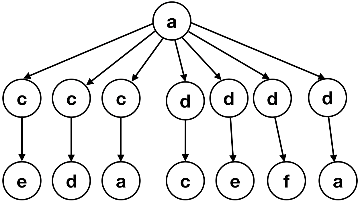
(b) Not the smallest possible

Figure 4. Trees having the required paths from the root to leaves, but not the valid 2-aggregation tree of $a$. Sub-figure (a) is not a valid arborescence since there should only be one path from the root to any node in an arborescence (Gordon and McMahon, 1989). Sub-figure (b) is a valid arborescence but not the smallest.

Figure 3 shows an example of a graph along with the various aggregation trees $T^{*}_{a}$ of the node $a$ in it. Figure 4 shows some trees that have the same root node and the same set of paths from the root to leaves but are not valid $2$-aggregation trees of node $a$. We would like to point out to the reader that the two assumptions we made for graphs are not upheld in the case of aggregation trees:

• Aggregation trees can contain multiple replicas of the same node (Shervashidze et al., 2011). For example, the $2$-aggregation tree $T^{2}_{a}$ shown in figure 3 has node $a$ as the root and also as two of the leaves. The replicas are treated as distinct nodes so that aggregation trees remain acyclic, but all of them correspond to the same node in the base graph.

• Aggregation trees are directed, making the notion of neighbor set different in their case than in the case of undirected graphs. In an aggregation tree, the neighbor set $\mathcal{N}_{v}$ of a node $v$ only contains those nodes that have incoming edges from $v$, but not those that have outgoing edges to $v$. Therefore, in the context of aggregation trees, we refer to the neighbor set of a node as its set of children or child set for clarity.

The two lemmas given below highlight some core properties of aggregation trees.

Lemma 3.2.

Given a $k$-aggregation tree $T^{k}_{v}$, let a subtree of $T^{k}_{v}$ be defined as any node along with all its descendants up to some depth $l$ ($l\leq k$). Then every subtree of $T^{k}_{v}$ is also an aggregation tree.

Proof. Let us assume that the subtree at some node $u$ in $T^{k}_{v}$ is not an aggregation tree. Then there exists a path in $T^{k}_{v}$ from the root $v$ to some leaf in it via $u$ that is not a $k$-length walk starting at node $v$ in the base graph, or vice versa. But this contradicts the definition of aggregation trees. Hence, such a subtree cannot exist. $\square$

Lemma 3.3.

Given a graph $G$, let $v$ be any node in it without loss of generality. The child set of any non-leaf node in $T^{k}_{v}$ is equal to the neighbor set of the corresponding node in $G$.

Proof. We prove this also by contradiction. A non-leaf node in $T^{k}_{v}$ must be reachable in at most $k-1$ hops from $v$ in $G$. Consequently, if there exists a non-leaf node in $T^{k}_{v}$ such that its child set is not equal to its corresponding neighbor set in $G$, then there exists a path from the root of $T^{k}_{v}$ to a leaf in it that is not a $K$-length walk in $G$, or vice versa. However, this contradicts the definition of $k$-aggregation trees. Hence, such a non-leaf node cannot exist. $\square$

3.2. Connection to aggregation-based GNNs

We now establish the connection between aggregation trees and aggregation-based GNNs.

Theorem 3.4.

Given a graph $G$, let $v$ be any node in it without loss of generality. The $k$-aggregation tree $T^{k}_{v}$ of $v$ denotes the structure captured by the representation $h^{(k)}_{v}$ computed using a $k$-layer aggregation-based GNN for $v$. Alternatively, a $k$-layer aggregation-based GNN, when applied to $T^{k}_{v}$, computes the same representation $h^{(k)}_{v}$ for root $v$ as it does for node $v$ when applied to $G$.

Proof. We prove this by induction on $k$. As per equation 1, when $k=1$, the computation of $h^{(1)}_{v}$ by a $1$-layer aggregation-based GNN is given by:

$$h^{(1)}_{v}=f^{(1)}\,\left(\,h^{(0)}_{v},\,g\,(\{h^{(0)}_{u}:u\in\mathcal{N}_{v}\})\,\right)$$

By lemma 3.3, we have that the child set of root $v$ in $T^{1}_{v}$ is identical to the neighbor set of $v$ in $G$. Furthermore, $h^{(0)}_{*}$ are the input feature vectors for nodes; any node in $T^{1}_{v}$ has the same $h^{(0)}_{*}$ as its corresponding node in $G$. So, the theorem trivially holds for $k=1$. Assume that the theorem also holds for some $k>1$, i.e., $h^{(k)}_{v}$ computed for root $v$ of $T^{k}_{v}$ by a $k$-layer aggregation-based GNN is identical to $h^{(k)}_{v}$ computed for node $v$ in $G$. Now, the computation of $h^{(k+1)}_{v}$ by a $k+1$-layer aggregation-based GNN is given by:

$$h^{(k+1)}_{v}=f^{(k+1)}\,\left(\,h^{(k)}_{v},\,g\,(\{h^{(k)}_{u}:u\in\mathcal{N}_{v}\})\,\right)$$

As before, we have that the child set of root $v$ in $T^{k+1}_{v}$ is identical to the neighbor set of $v$ in $G$. Additionally, the representations $h^{(k)}_{*}$ for root $v$ and its children capture the respective subtrees of depth $k$ under them. Since, these subtrees are actually $k$-aggregation trees (lemma 3.2), following our assumption, $h^{(k)}_{*}$ must be the same for root $v$ and its children as for the corresponding nodes in $G$. So, the theorem holds for $k+1$ when it holds for $k$ because inputs to the computation of $h^{(k+1)}_{v}$ are the same in the case of $T^{k+1}_{v}$ and $G$. Hence, the theorem holds for $k>=1$. $\square$

Essentially, the $k$-aggregation tree $T^{k}_{v}$ is a visual depiction of the representation $h^{(k)}_{v}$ computed by a $k$-layer aggregation-based GNN. Every subtree in $T^{k}_{v}$ is the depiction of some representation $h^{(l)}_{*}$ ($l<k$) computed intermediately.

4. Analysis of aggregation-based GNNs

Aggregation trees surface two important issues stemming from the way that aggregation-based GNNs operate.

The first one concerns the generalization ability of these architectures. When computing the representation $h^{(k)}_{v}$, a $k$-layer aggregation-based GNN with $k>1$ aggregates from the same set of nodes multiple times, especially from $v$ itself. An example of this can be seen in figure 3 where the node $a$ appears multiple times in its own $2$-aggregation tree $T^{2}_{a}$. Such repetitions allow the GNN to amplify the interactions (i.e., the message passing) between nodes and their neighbors, which has two known downsides (Rong et al., 2020): 1) it facilitates over-smoothing whereby representations of nodes within a neighborhood become indistinguishable despite belonging to different classes, and 2) it results in over-fitting whereby the GNN cannot generalize well beyond training. In fact, Wang et al. (Wang et al., 2019) even present empirical observations of over-smoothing in GAT.

The second issue pertains to scalability of a $k$-layer aggregation-based GNN where $k>1$. In many real-world settings, there is a large graph that keeps growing with time. A prime example is social networks where new users join from time to time. In such settings, learning follows the inductive paradigm whereby we train the GNN on a snapshot of the graph in time, and then predict on new nodes that enter the graph after that. Figure 5(a) depicts such a setting where $v$ is a node entering the graph after training. Figure 5(b) shows the $k$-aggregation tree $T^{k}_{v}$, i.e., the structure that will be captured by the representation $h^{(k)}_{v}$. Essentially, the GNN requires input vectors $h^{(0)}_{*}$ for all the nodes within $k$ hops of $v$ to compute $h^{(k)}_{v}$. This can be up to $\mathcal{O}(d^{k})$ representations in total, where $d$ is the average degree of a node.

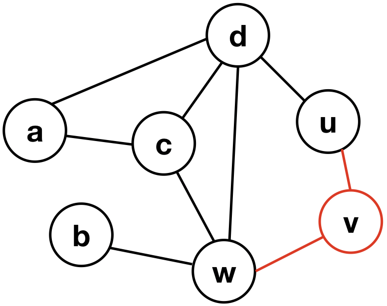
(a) Node $v$ enters the graph post training

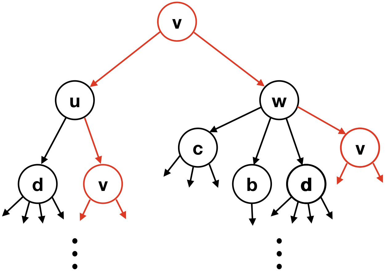
(b) $T^{k}_{v}$, the $k$-aggregation tree of $v$

Figure 5. Depiction of the scenario where a node $v$ enters a graph at prediction time after training has finished. The $k$-aggregation tree of node $v$ is also shown.

Storing representations from layers of a GNN has been explored as an optimization before (Chen et al., 2018). In the example above, the representations $h^{(*)}_{u}$ and $h^{(*)}_{w}$ can be cached at the end of training since they capture the relevant aggregation trees of $u$ and $w$ respectively. Then the representation $\hat{h}^{(k)}_{v}$ can be approximated at prediction time as:

(4) $$\hat{h}^{(k)}_{v}=f^{(k)}\,\left(\,\hat{h}^{(k-1)}_{v},\,g\,(\{\tilde{h}^{(k-1)}_{u}:u\in\mathcal{N}_{v}\})\,\right)$$

where $\tilde{h}$ denotes the cached representations, and $\hat{h}$ signifies that the computed representation is an approximation of $h^{(k)}_{v}$. The $k$-aggregation tree for equation 4 is shown in figure 6. Note that, unlike 5(b), now $v$ only appears as the root, making $h^{(k)}_{v}$ and $\hat{h}^{(k)}_{v}$ different. This is because $v$ was not present during training, and consequently, not covered by the cached representations.

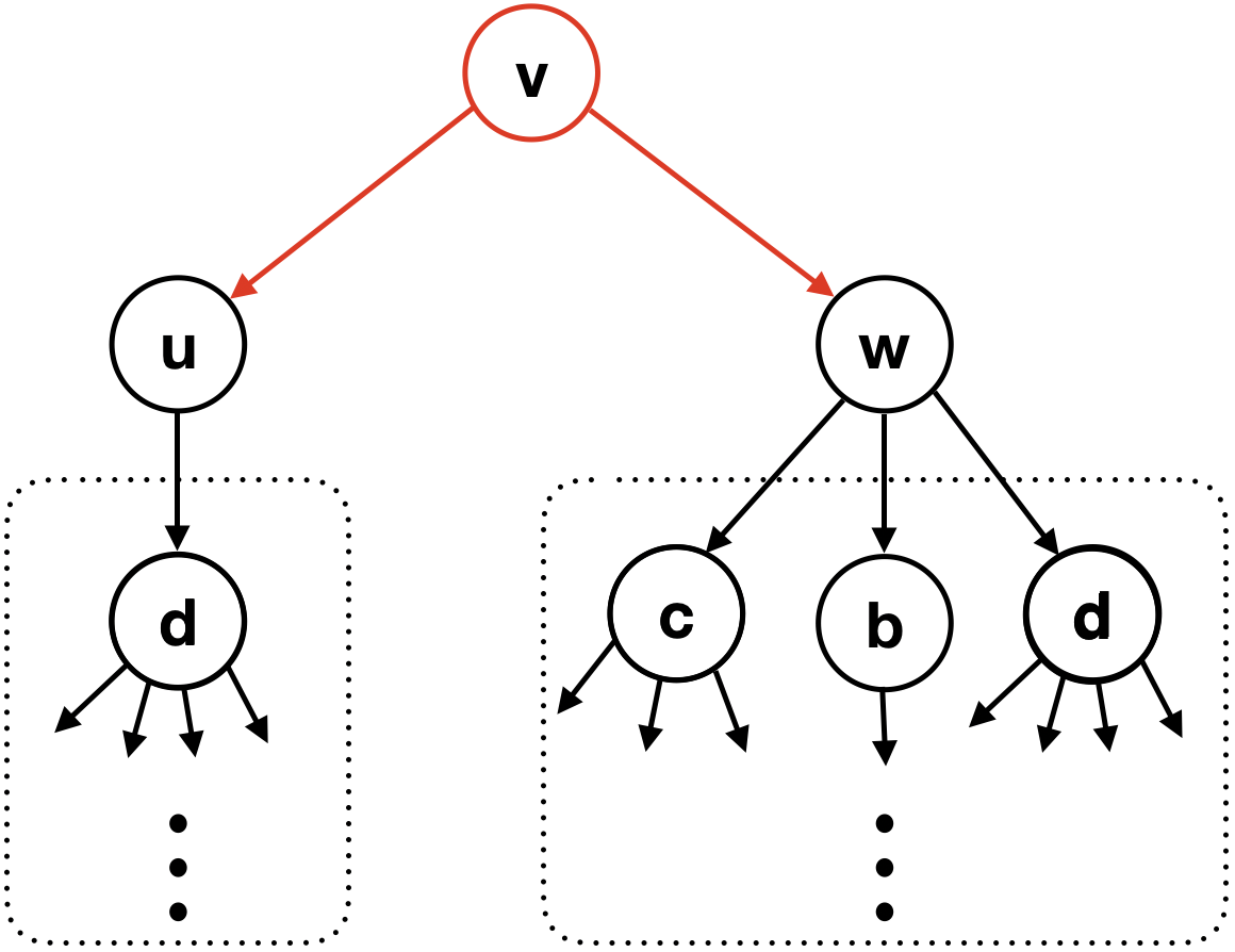
Figure 6. The $k$-aggregation tree of node $v$ as per equation 4. The dotted boxes encapsulate the aggregation trees captured by cached representations $\tilde{h}^{(1)}_{*}$, $\dots$, $\tilde{h}^{(k-1)}_{*}$ for $u$ and $w$.

Essentially, with caching, the GNN only requires the $k$ representations $\tilde{h}^{(0)}_{*}$, $\dots$, $\tilde{h}^{(k-1)}_{*}$ for every 1-hop neighbor of $v$ to approximate $h^{(k)}_{v}$, i.e., up to $\mathcal{O}(kd)$ representations in total. While this is a substantial gain in efficiency, we show empirically in section 6 that the performance at prediction suffers given that the structure of aggregation trees differs between training and prediction times.

5. Node Masking

We propose node masking as a novel yet simple training phase technique to address the issues highlighted in the previous section.

5.1. Description

We begin by formalizing the notion of a masking function for generic countable sets.

Definition 5.1.

Let $\mathcal{S}$ be a set of elements; we assume $\mathcal{S}$ is countable. Let $\mathcal{B}^{n}_{p}$ be the set of outputs of $n$ Bernoulli trials ($n=|\mathcal{S}|)$ with probability $p$ of success. We define $\delta_{p}$ to be a bijective mapping from $\mathcal{S}$ to $\mathcal{B}^{n}_{p}$, and refer to it as the Bernoulli select function. There can be $n!$ different $\delta_{p}$. Now, the masking function $\mathcal{M}$ can be defined for $\mathcal{S}$ and a $\delta_{p}$ as:

(5) $$\mathcal{M}(\mathcal{S},\delta_{p})=\{e:e\in\mathcal{S},\,\delta_{p}(e)=1\}$$

Here, all the elements $e$ with $\delta_{p}(e)=0$ are said to be masked. Next, we demonstrate how we inculcate this masking function $\mathcal{M}$ in the computations of aggregation-based GNNs to tackle the issues we discussed in the previous section. Let $\delta^{G}_{p}$ be the Bernoulli select function over the set of nodes of a given graph $G$. We propose node masking as the following modification to equation 1 that defines the update operation in the $k^{th}$ layer of an aggregation-based GNN:

(6) $$h^{(k)}_{v}=f^{(k)}\bigg{(}h^{(k-1)}_{v},g\Big{(}\{h^{(k-1)}_{u}:u\in\mathcal{M}(\mathcal{N}_{v},\delta^{G}_{p})\}\Big{)}\bigg{)}$$

We refer to $p$ as the node masking rate. If $p$ is set to 1 in $\delta^{G}_{p}$, then equation 6 resembles equation 1, i.e., node masking has no effect. Thus, we say node masking is inactive when $p=1$ and active when $p<1$.

The actual implementation of node masking may vary across the different aggregation-based GNNs. Equations 7 and 8 lay out the implementations of node masking in GAT and GIN-0 (Xu et al., 2019) architectures respectively:

(7) $$h^{(k)}_{v}=\bigg{\|}_{l}\,\sigma\left(\,\sum_{u}^{v\,\cup\,\mathcal{N}_{v}}\delta^{G}_{p}(u)\cdot\alpha^{(k)}_{l}(v,u)\cdot W^{(k)}_{l}h^{(k-1)}_{u}\,\right)$$

(8) $$h^{(k)}_{v}=MLP^{(k)}\,\left(h^{(k-1)}_{v}+\,\sum_{u}^{\mathcal{N}_{v}}\,\delta^{G}_{p}(u)\cdot h^{(k-1)}_{u}\,\right)$$

In both cases, any node $u$ with $\delta^{G}_{p}(u)=0$ is effectively masked since its contribution to the sum is nullified.

Essentially, given a graph $G$ and a $k$-layer aggregation-based GNN, if a node $v$ in $G$ is masked, then the representations $h^{(l)}_{v}$ ($l<k$) are discarded during the computations performed by the GNN. The equivalent effect in aggregation trees is that $v$ is is not included in the child set of other nodes in any aggregation tree since it cannot contribute to representations of other nodes. Going back to the example graph in figure 3, figure 7 shows some possible $2$-aggregation trees $T^{2}_{a}$ of the node $a$ depending on the nodes that are masked. Note, even if a node is masked, it can still appear as the root of its own aggregation tree since root is not in any child set.

(a) No nodes masked

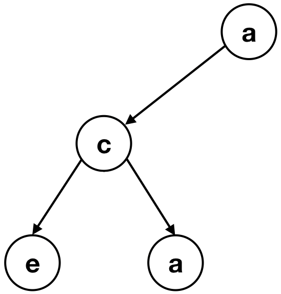
(b) Node $d$ is masked

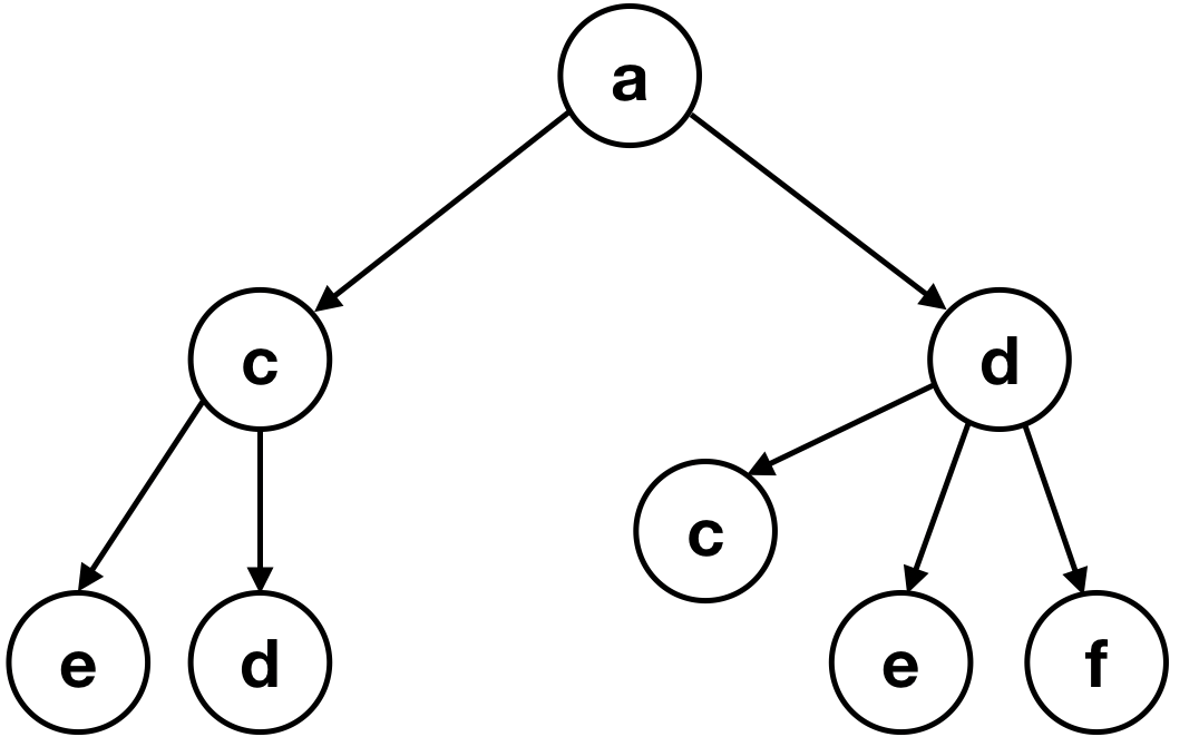
(c) Node $a$ is masked

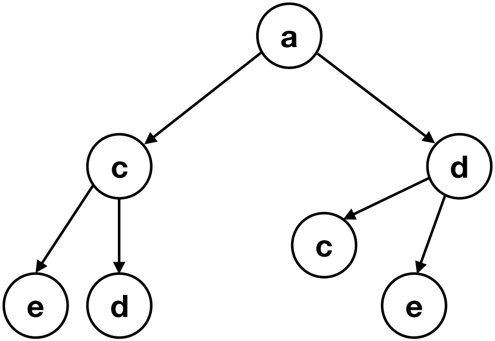
(d) Nodes $a$ and $f$ are masked

Figure 7. Some possible $2$-aggregation trees $T^{2}_{a}$ of node $a$ in the base graph shown by figure 3(a). The aggregation trees vary based on the nodes that are masked. If a node is masked, it is excluded from the child set of other nodes but can still appear as the root.

When a $k$-layer aggregation-based GNN with active node masking is trained on some graph $G$, a Bernoulli select function $\delta^{G}_{p}$ is randomly sampled in every training epoch, allowing the GNN to see many different $T^{k}_{v}$ for every node $v$. This has two advantages. First, the GNN is discouraged from simply associating a node and its neighbors together. Second, if $\delta^{G}_{p}(v)=0$ in an epoch, then $T^{k}_{v}$ has the same structure as the aggregation tree in figure 6, i.e., no repetition of $v$ in $T^{k}_{v}$. This reduces the tendency of the GNN to focus heavily on $v$’s own features and also sensitizes the GNN to that structure of the aggregation trees that it may encounter at prediction time if caching is used.

In summary, node masking can be seen a training phase technique for GNNs that stresses the relational inductive biases in the data, while also having a regularizing effect that prevents aggregation-based GNNs from easily amplifying the interactions between nodes and their neighbors, hence alleviating over-fitting and over-smoothing. Once training has finished, node masking can easily be inactivated by setting the node masking rate $p$ to 1.

5.2. Node masking vs. Dropout techniques

Recently, quite a few works have explored ideas around stochastically dropping nodes and edges within GNN layers using Dropout (Srivastava et al., 2014). Rong et al. (Rong et al., 2020) proposed the concept of DropEdge in spectral GNNs to alleviate the problem of over-fitting and over-smoothing. DropEdge randomly drops a subset of edges from the graph in every training epoch. In the GAT paper (Veličković et al., 2018), the authors employed a similar technique by applying dropout to the attention coefficients within each GAT layer, which made the learning process more robust to over-fitting. However, neither of these techniques systematically addresses the problem of repetition in aggregation trees and neither of them facilitates caching. In fact, we show in our experiments that the GAT architecture performs much better when node masking is used instead of dropout on attention coefficients.

6. Experiments

To empirically verify the theory we have discussed up till now, we conduct over 200 experimental runs, covering both the aspects we highlighted, i.e., generalization and scalability.

6.1. Datasets

We work with three widely-used benchmark datasets for node classification: the Cora and PubMed citation networks (Sen et al., 2008) and the social network graph of Reddit posts (Hamilton et al., 2017). We pick these datasets since they are the ones used across several works that explore over-fitting and over-smoothing in GNNs (Wang et al., 2019; Rong et al., 2020; Li et al., 2018; Chen et al., 2020).

Cora. The Cora citation network dataset consists of $2,708$ nodes and $5,429$ edges. Nodes denote scientific publications and edges denote the citation relationships amongst them. Note that the edges are undirected for the purpose of the dataset even though citations are not symmetric (Kipf and Welling, 2017; Veličković et al., 2018). The publications are represented as binary bag-of-words vectors consisting of 1433 features each. Every node belongs to one of the seven classes, indicating the area of publication, e.g., Genetic Algorithms or Reinforcement Learning.

PubMed. The PubMed diabetes dataset consists of $19,717$ nodes and $44,338$ edges. Nodes denote scientific publications on diabetes and edges denote the citation relationships amongst them. As above, the edges are undirected for the purpose of the dataset. The publications are represented as TF-IDF weighted bag-of-words feature vectors with 500 features each. Every node belongs to one of the three classes, indicating the type of diabetes that the publication is about, e.g., Diabetes Mellitus Type 1 or Diabetes Mellitus Type 2.

Reddit. The Reddit posts graph consists of $232,965$ nodes denoting posts from $41$ different sub-reddits. An undirected edge is present between two posts if the same user(s) commented on the two posts. Each post is represented by a $602$-dimensional feature vector formed by concatenating distributional semantic features and count-based features for title and comments.

6.2. Models and configurations

We experiment with both of the aggregation-based GNNs that we have discussed up till now, i.e., GAT and GIN. For the GIN architecture, we utilize the formulation specified by equation 7. If node masking is inactive, this formulation behaves exactly like the GIN-0 architecture from the original paper (Xu et al., 2019) that was shown to have state of the art performance. For the GAT architecture, we use the original formulation (Veličković et al., 2018) specified by equation 2. Additionally, we define a variant of GAT that we refer to as simple GAT or SGAT:

(9) $$h^{(k)}_{v}=\bigg{\|}_{l}\,\sigma\left(\,\sum_{u}^{v\,\cup\,\mathcal{N}_{v}}\frac{\delta^{G}_{p}(u)}{|v\cup\mathcal{N}_{v}|}\cdot W^{(k)}_{l}h^{(k-1)}_{u}\,\right)$$

When node masking is inactive, this variant behaves exactly like the original GAT architecture except that the attention coefficients are now simply the inverse of a node’s degree.

6.3. Experimental settings

We use PyTorch (Paszke et al., 2019) for modeling. For the GAT and SGAT architectures, we set the exact same hyper-parameters as in the original paper (Veličković et al., 2018) for the Cora dataset. We do not experiment with GAT and SGAT on the PubMed and Reddit datasets because that requires support for operations like sparse softmax (Veličković et al., 2018), which are not stable in PyTorch yet. Akin to GAT, we found a 2-layer GIN to be optimal for all the datasets. We set the maximum number of epochs to $1,000$ with an early stopping patience of $50$ epochs. We use the Adam optimizer (Kingma and Ba, 2015) to update the parameters. If node masking is active, then in every training epoch, we randomly sample a Bernoulli select function over the nodes in the train set. Node masking is always inactive outside training. We submit our code for further reference.

We experiment with both transductive and inductive learning paradigms. In the transductive setting, we make the entire graph from the dataset available at training time, i.e., all the nodes and edges. That said, the the loss for back-propagation is calculated using labels on the nodes in the train set only. In the inductive setting, we only make available at training time the graph $\mathcal{G}$ formed by nodes in the train set plus the edges amongst them. At validation and test times, we introduce the relevant nodes from the dataset into $\mathcal{G}$ along with the corresponding edges.

Unlike previous works, which test their hypotheses only on a single split of the datasets, we experiment with multiple splits of the three datasets in both the transductive and inductive settings. Specifically, for each dataset, we experiment with 10%, 20%, 25%, 33%, 50%, 75%, and 90% of the nodes as the train set. In all the cases, the remaining data forms our test set except for a small part that we designate as the validation set for evaluating the early stopping criterion in the training phase. For every split, we perform stratified partitioning of the data to ensure similar class distribution.

Note that the metrics we present from our experiments are all in fact mean metrics over 10 trials with random initializations of the parameters. Unlike previous works that use micro F₁ and accuracy, we report macro F₁ since we strongly consider it to be a more appropriate metric as it provides an equal evaluation of effectiveness on all classes (Van Asch, 2013). That said, we noted that all the trends are consistent with micro F₁ and accuracy too.

6.4. Generalization

To show that node masking helps aggregation-based GNNs generalize better, we compare the performances yielded by the models when node masking is active versus when it is inactive. We denote the configurations where node masking is active by “+NM” and use a consistent rate of $p=0.5$. That said, $p$ is a hyper-parameter that can be adjusted for further gains. Appendix A explores the change in performance as $p$ and number of layers in the GNN vary.

Table 1. Macro F₁ scores on the Cora dataset in inductive and transductive settings for various sizes s of the train set (in percentage). Numbers in bold are significantly better than their counterparts with $p$-value $<0.05$ under paired t-test.

	s	gat	gat+nm	sgat	sgat+nm
	10	40.74	51.25	40.57	50.64
	20	68.40	74.65	68.50	74.82
	25	74.12	78.71	74.34	79.32
Inductive	33	80.44	82.56	80.30	82.74
	50	84.77	85.52	85.04	85.44
	75	87.00	87.03	87.16	87.29
	90	86.86	86.72	86.46	86.94
	10	82.01	82.77	82.17	83.46
	20	84.20	85.04	84.35	85.34
	25	84.95	85.38	85.12	85.88
Transductive	33	85.87	86.35	85.86	86.72
	50	86.61	87.35	87.32	87.61
	75	87.93	88.18	88.43	88.44
	90	87.25	87.36	87.24	87.22

Table 1 shows the comparisons between GAT and GAT+NM and between SGAT and SGAT+NM on the Cora dataset. GAT+NM and SGAT+NM outperform their counterparts across several splits in both the transductive and inductive settings. As expected, the gains are more pronounced in the inductive setting and amongst smaller sizes of the train set. Note that in GAT+NM and SGAT+NM, we do not use any dropout on the attention coefficients. So, the wins over GAT and SGAT clearly indicate that node masking is more effective than stochastically dropping edges because the latter does not systematically address the issue of repetition of nodes in aggregation trees. More specifically, dropout-based techniques simply make the aggregation trees sparser but do not strongly impede amplified interactions between nodes and their neighbors.

We further validate our reasoning by calculating the Mean Average Distance (MAD) values for the GAT and SGAT models with and without node masking. MAD is a metric recently proposed by Chen et al. (Chen et al., 2020) that quantifies the smoothing caused by a GNN by computing a cosine distance based scalar measure over the representations generated for all the nodes in a graph. The lower the MAD value, the higher the smoothing caused by the GNN. Table 2 presents the MAD values on the Cora dataset. We see that node masking is significantly better at alleviating over-smoothing than the stochastic exclusion of edges. These results are in line with the observations of Wang et al. (Wang et al., 2019) who found the dropout on attention coefficients to not be a very effective tool against over-smoothing.

Table 2. MAD values on the Cora dataset in inductive and transductive settings with a train set of size 10%. Numbers in bold are significantly better than their counterparts with $p$-value $<0.05$ under paired t-test.

	Inductive	Transductive
gat (-attn. dropout)	0.20	0.46
gat	0.23	0.52
gat + nm	0.29	0.57
sgat (-attn. dropout)	0.20	0.44
sgat	0.24	0.51
sgat + nm	0.27	0.56

Tables 8(a), 8(b) and 8(c) compare GIN and GIN+NM on the Cora, PubMed and Reddit datasets respectively. Again, node masking helps boost performance across almost all splits in both the transductive and inductive settings. Note that, due to the size of the Reddit dataset, we could not run the experiments in transductive setting or inductive setting with train set $>50\%$ on our machines with NVIDIA P100 GPUs. Other works (Rong et al., 2020) have noted the same.

Table 3. Macro F₁ scores on the Cora, PubMed and Reddit datasets in inductive and transductive settings for various sizes s of the train set (in percentage). Numbers in bold are significantly better than their counterparts with $p$-value $<0.05$ under paired t-test.

	Inductive		Transductive
s	gin	gin+nm	gin	gin+nm
10	52.91	56.38	77.95	79.65
20	71.10	74.38	81.65	82.66
25	74.71	77.94	82.72	83.87
33	78.84	80.98	83.78	84.61
50	83.07	84.49	85.63	86.57
75	85.46	86.88	87.40	87.91
90	85.13	86.63	86.67	87.82

(a) Cora

	Inductive		Transductive
s	gin	gin+nm	gin	gin+nm
10	77.51	78.31	83.65	84.34
20	82.11	82.86	84.61	85.20
25	82.95	83.94	85.03	85.47
33	83.78	84.46	85.35	85.84
50	85.25	85.79	85.89	86.42
75	85.99	86.53	86.38	86.55
90	86.42	86.80	86.43	86.61

(b) PubMed

	Inductive
s	gin	gin+nm
10	78.12	87.09
20	83.38	87.73
25	86.76	88.74
33	87.57	88.94
50	88.93	90.97

(c) Reddit

We found the MAD values for GIN and GIN+NM to be almost identical, e.g., 0.65 for Cora with a train set of size 10%. This is intuitive given that GIN is a maximally powerful GNN that, in theory, can achieve injective mapping from nodes to representations (Xu et al., 2019). However, injectivity can lead to over-fitting (Seo et al., 2019), which node masking counters by stochastically augmenting the training graph to stress the relational inductive biases. We validate this by presenting some loss curves in appendix B on the Cora and PubMed datasets with and without node masking under transductive and inductive settings. They highlight the regularizing effect of node masking.

6.5. Scalability

Tables 8(d) and 8(e) compare the performances of GIN on the Cora and PubMed datasets respectively with and without caching. For both the settings, each table also shows the number of unique nodes involved in the computations done by the model to generate predictions for the nodes introduced into the graph at the test time. Caching consistently reduces the number of unique nodes involved because only those nodes from the train set need to be involved that are 1-hop neighbors of the nodes introduced at the test time. The gains in efficiency from caching are more pronounced when the number of nodes present at the training time is significantly more than the number of nodes entering at the test time, a common scenario in the real-world. However, as conjectured before, the model performs worse with caching because the structure of aggregation trees it captures at the test time differs from the structure it learned to capture at the training time. That said, when node masking is used, the performance in fact exceeds that of GIN without caching.

Table 4. Macro F₁ scores on the Cora and PubMed datasets in inductive setting with and without caching for various sizes s of the train set (in percentage). F₁ scores in bold are significantly better than their counterparts with $p$-value $<0.05$ under paired t-test.

	GIN		GIN + Caching
s	f1	#nodes	f1	f1 (+nm)	#nodes
10	52.91	2708	51.89	55.82	2698
20	71.10	2708	69.59	74.17	2672
25	74.71	2708	73.55	77.32	2644
33	78.84	2708	77.60	80.72	2605
50	83.07	2708	82.50	83.95	2426
75	85.46	2708	84.90	86.59	1781
90	85.13	2708	84.81	85.85	919

(d) Cora

	GIN		GIN + Caching
s	f1	#nodes	f1	f1 (+nm)	#nodes
10	77.51	19717	76.25	78.33	19614
20	82.11	19717	81.47	82.75	19300
25	82.95	19717	82.24	83.77	19059
33	83.78	19717	82.83	84.15	18553
50	85.25	19717	84.27	85.34	16733
75	85.99	19717	85.46	86.01	11944
90	86.42	19717	85.87	86.61	6682

(e) PubMed

Here, one might seek a comparison with GraphSAGE (Hamilton et al., 2017) which reduces the number of unique nodes involved in the computation of $h^{k}_{v}$ for a node $v$ by sub-sampling its $k$-hop neighborhood. Such sub-sampling, however, makes GraphSAGE lose a lot of information, rendering it worse than aggregation-based GNNs on these benchmark datasets (Shchur et al., 2018). We instead reduce the number of unique nodes involved in the computation carried out by aggregation-based GNNs by approximating $h^{k}_{v}$ using the cached representations of 1-hop neighbors of $v$. This approximation does not degrade the performance when node masking is employed.

7. Conclusion

In this paper, we introduced node masking, a novel technique that significantly improves the performance of state of the art graph neural networks (GNNs). We first discussed some theoretical tools to better visualize the operations performed by spatial aggregation-based GNNs. Using these tools, we highlighted the issues that limit the ability of such GNNs to generalize and scale. Finally, we empirically demonstrated the effectiveness of node masking in enhancing the performance of aggregation-based GNNs on three widely-used benchmark datasets for node classification, the Cora and PubMed citation network and the social network graph of Reddit posts. The observed trends also hold for the CiteSeer dataset but we omitted it for brevity. Previous works utilizing these datasets had tested their hypotheses only on a single split of the datasets. We instead showed the efficacy of node masking on a range of splits under both the transductive setting as well as the inductive setting, hence laying down strong benchmarks for future research.

Appendix A Varying the node masking rate

The analyses presented in this section are with the Cora dataset but the observed trends hold across all the datasets.

Figures 8 and 9 explore the change in performance of GIN+NM, GAT+NM, and SGAT+NM as the node masking rate $p$ increases from 0.1 up to 0.9. We conduct the experiments on the Cora dataset with a train set of size 10%.

As seen in figure 8, GIN+NM achieves the best performance under both the transductive setting as well as the inductive setting at $p>0.5$. This suggests that fine-tuning the node masking rate $p$ can yield even higher gains than we report in the paper. On the hand, figure 9 suggests that GAT+NM and SGAT+NM achieve the best performance at $p=0.5$ only.

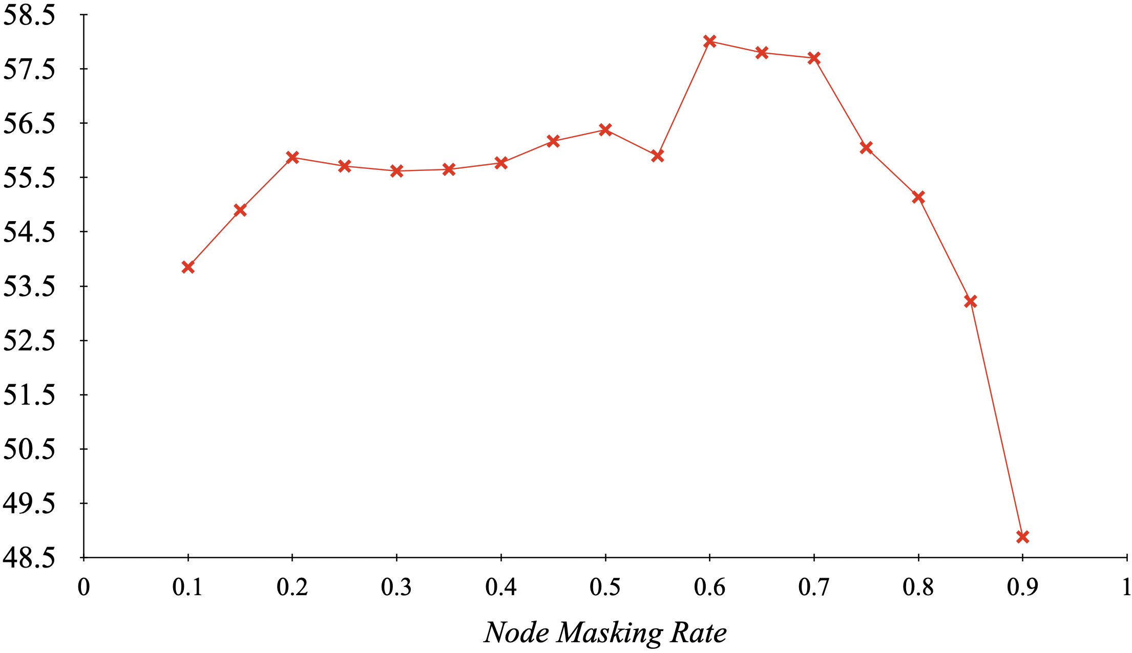
(f) GIN+NM in inductive setting

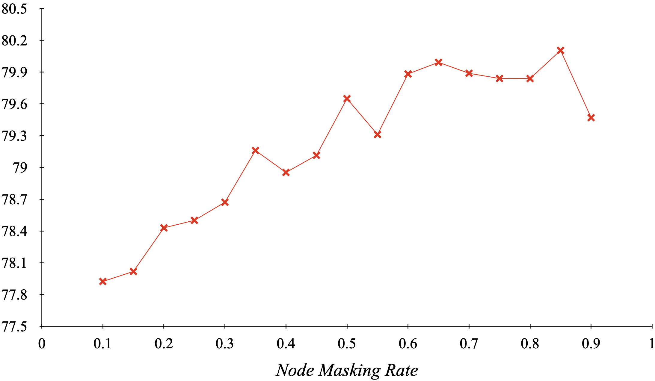
(g) GIN+NM in transductive setting

Figure 8. Results on the Cora dataset with GIN+NM under both the inductive and transductive settings for various node masking rates $p\in[0.1,0.9]$. The train set size is 10%. Y-axis denotes macro F₁. We see that the best performance is not necessarily with $p=0.5$.

Figure 10 further explores how the performance of GIN+NM changes with varying node masking rates $p$ when the number of GNN layers, i.e., the depth of the model, is increased from 2 to 4, 8 or 16. We note that as the depth increases, the $p$ at which the optimal performance is achieved decreases. This is intuitive given that more layers means more parameters, which in turn means denser aggregation trees are required for optimal training.

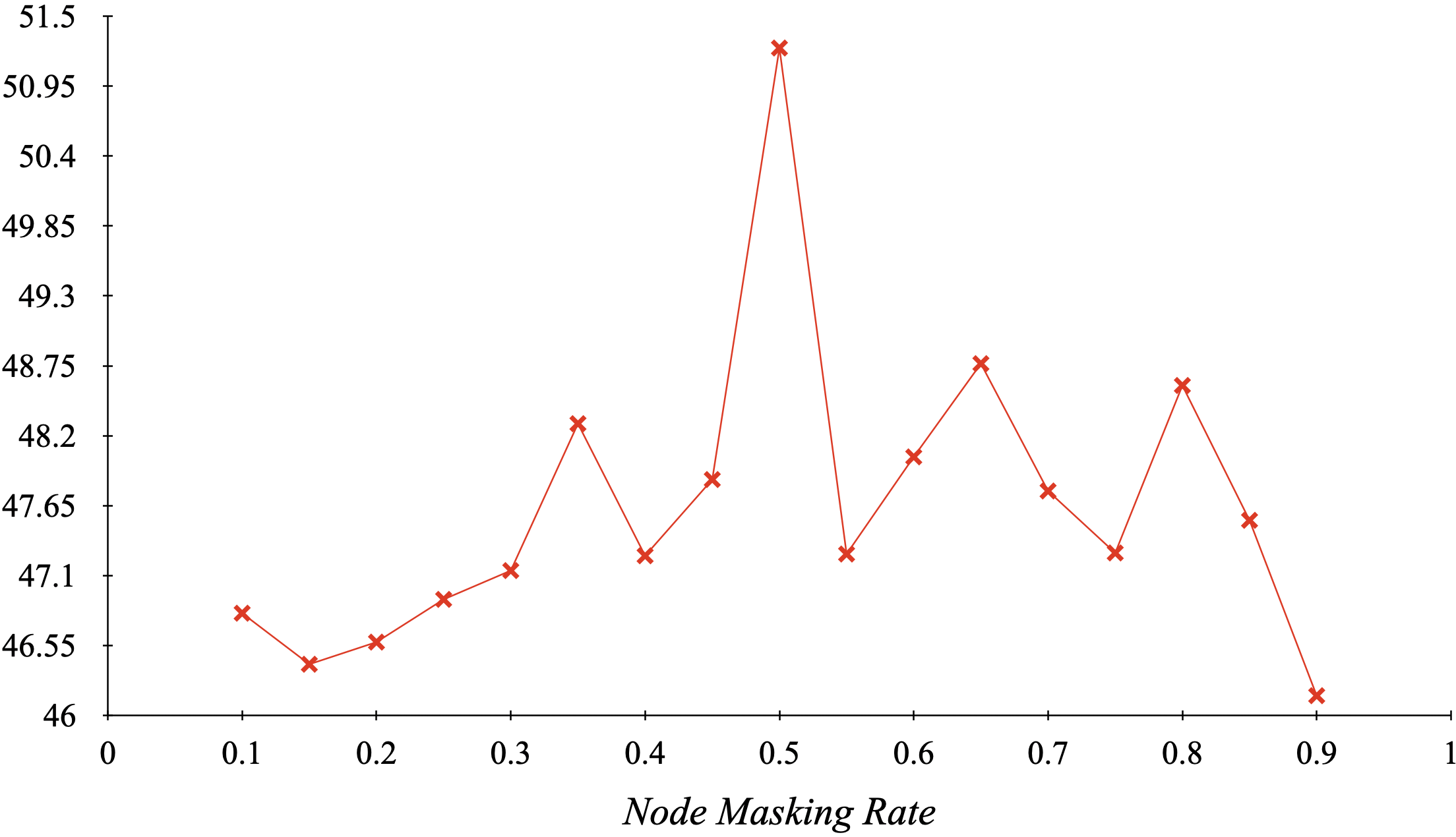
(a) GAT+NM in inductive setting

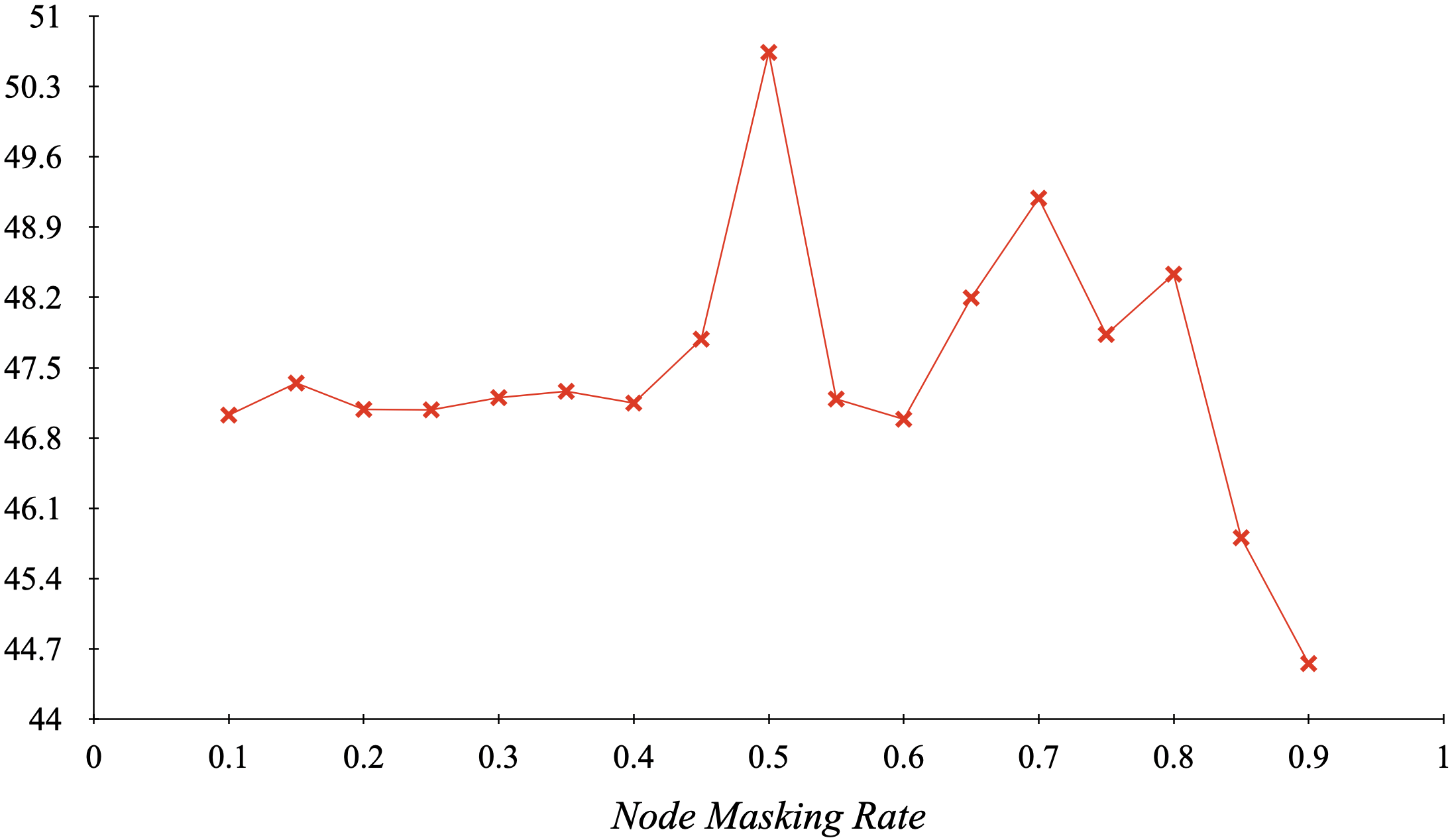
(b) SGAT+NM in inductive setting

Figure 9. Results on the Cora dataset with GAT+NM and SGAT+NM under inductive setting for various node masking rates $p\in[0.1,0.9]$. The train set size is 10%. Y-axis denotes macro F₁. We see that the best performance is with $p=0.5$.

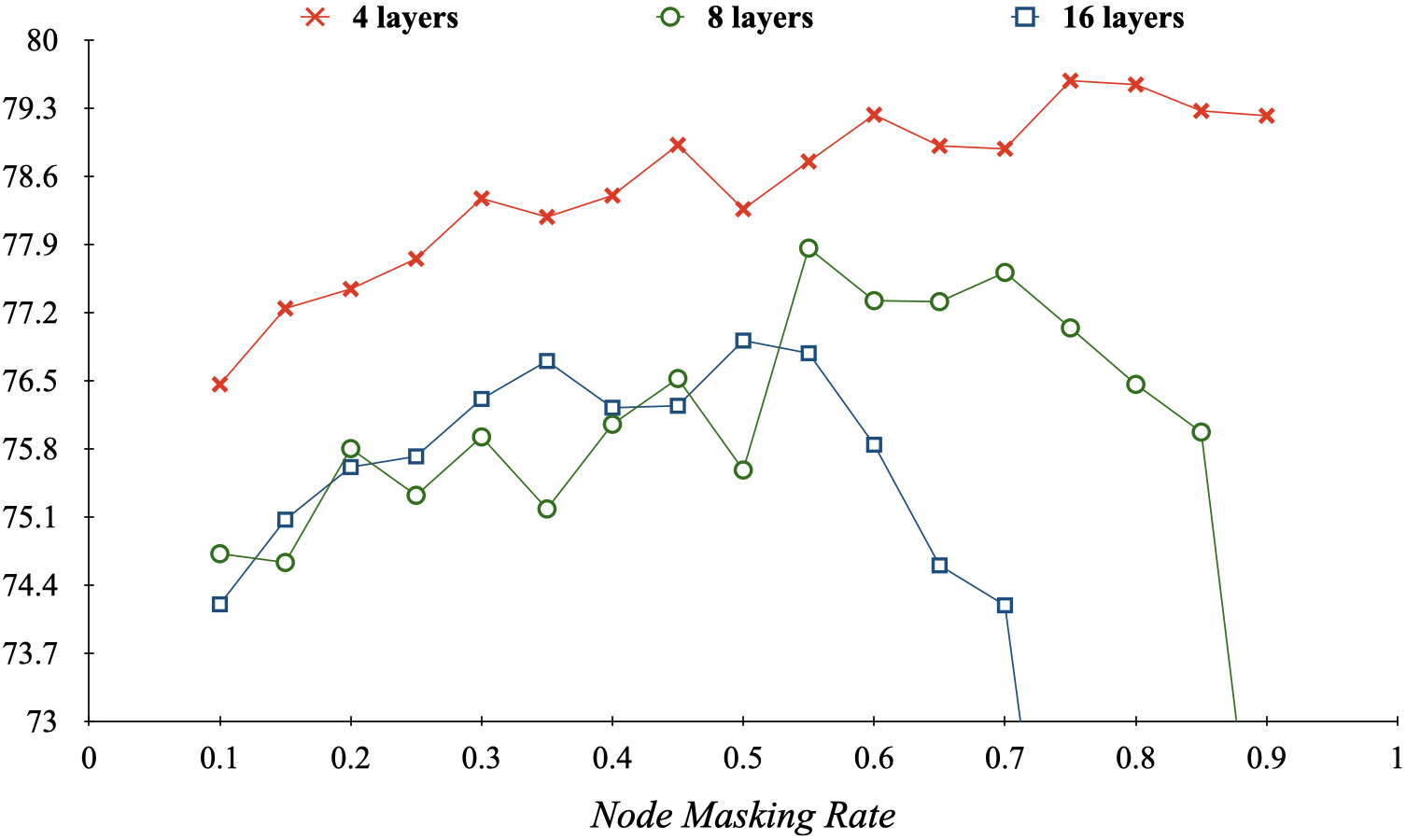
Figure 10. Results on the Cora dataset with GIN+NM under the transductive setting for various node masking rates $p\in[0.1,0.9]$ and depths of the model. The train set size is 10%. Y-axis denotes macro F₁. We see that the $p$ at which the optimal performance is achieved decreases with increasing depth.

Appendix B Analysis of loss curves

Figures 11 and 12 present some loss curves from the training and validation phases for the GIN model with (green) and without (red) node masking under both the transductive and inductive settings.

(a) Loss curves on nodes in the train set

(b) Loss curves on nodes in the validation set

Figure 11. Loss curves on the Cora dataset for the GIN model with (w/ NM) and without (w/o NM) node masking.

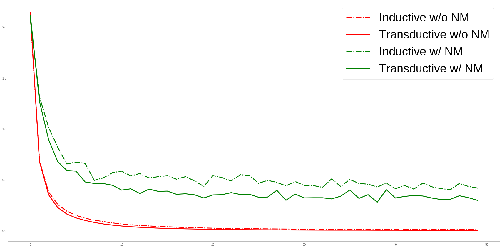
(a) Loss curves on nodes in the train set

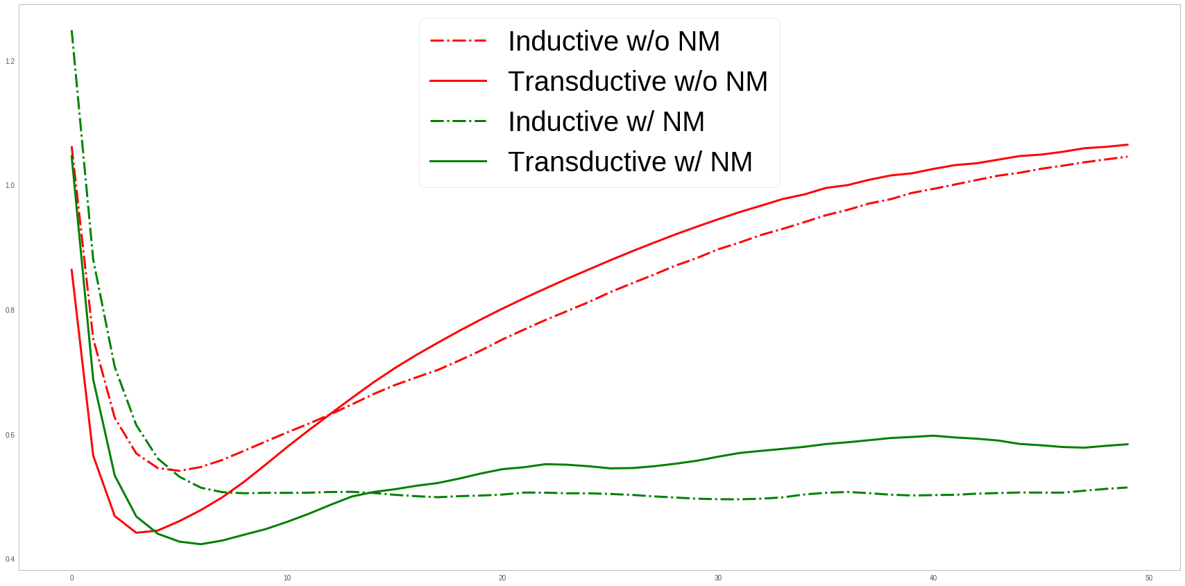
(b) Loss curves on nodes in the validation set

Figure 12. Loss curves on the PubMed dataset for the GIN model with (w/ NM) and without (w/o NM) node masking.

As can be noted, node masking leads to higher training losses in both the transductive and inductive settings. This is typical of a regularization effect. Additionally, we also observe that the validation losses go up sharply after a point when node masking is not used, clearly indicating that the model has over-fit. With node masking, such an over-fitting phenomenon is neither observed in the transductive setting nor in the inductive setting. Therefore, the model is able to achieve a lower validation loss meaning that it generalizes better. This is typical of a higher inductive bias effect.

References

- (1)
- Bach (2008) Francis R. Bach. 2008. Graph Kernels between Point Clouds. In Proceedings of the 25th International Conference on Machine Learning (Helsinki, Finland) (ICML ’08). Association for Computing Machinery, New York, NY, USA, 25–32. https://doi.org/10.1145/1390156.1390160
- Battaglia et al. (2018) Peter W. Battaglia, Jessica B. Hamrick, Victor Bapst, Alvaro Sanchez-Gonzalez, Vinícius Flores Zambaldi, Mateusz Malinowski, Andrea Tacchetti, David Raposo, Adam Santoro, Ryan Faulkner, Çaglar Gülçehre, H. Francis Song, Andrew J. Ballard, Justin Gilmer, George E. Dahl, Ashish Vaswani, Kelsey R. Allen, Charles Nash, Victoria Langston, Chris Dyer, Nicolas Heess, Daan Wierstra, Pushmeet Kohli, Matthew Botvinick, Oriol Vinyals, Yujia Li, and Razvan Pascanu. 2018. Relational inductive biases, deep learning, and graph networks. CoRR abs/1806.01261 (2018). arXiv:1806.01261 http://arxiv.org/abs/1806.01261
- Bruna et al. (2014) Joan Bruna, Wojciech Zaremba, Arthur Szlam, and Yann LeCun. 2014. Spectral Networks and Locally Connected Networks on Graphs. In 2nd International Conference on Learning Representations, ICLR 2014, Banff, AB, Canada, April 14-16, 2014, Conference Track Proceedings, Yoshua Bengio and Yann LeCun (Eds.). http://arxiv.org/abs/1312.6203
- Chen et al. (2020) Deli Chen, Yankai Lin, Wei Li, Peng Li, Jie Zhou, and Xu Sun. 2020. Measuring and Relieving the Over-Smoothing Problem for Graph Neural Networks from the Topological View. Proceedings of the AAAI Conference on Artificial Intelligence 34, 04 (Apr. 2020), 3438–3445. https://doi.org/10.1609/aaai.v34i04.5747
- Chen et al. (2018) Jianfei Chen, Jun Zhu, and Le Song. 2018. Stochastic Training of Graph Convolutional Networks with Variance Reduction. In International Conference on Machine Learning. 941–949.
- Chiang et al. (2019) Wei-Lin Chiang, Xuanqing Liu, Si Si, Yang Li, Samy Bengio, and Cho-Jui Hsieh. 2019. Cluster-GCN: An Efficient Algorithm for Training Deep and Large Graph Convolutional Networks. In ACM SIGKDD Conference on Knowledge Discovery and Data Mining (KDD). https://arxiv.org/pdf/1905.07953.pdf
- Defferrard et al. (2016) Michaël Defferrard, Xavier Bresson, and Pierre Vandergheynst. 2016. Convolutional neural networks on graphs with fast localized spectral filtering. In NIPS. 3844–3852.
- Fournier (2013) Jean-Claude Fournier. 2013. Graphs theory and applications: with exercises and problems. John Wiley & Sons.
- Gordon and McMahon (1989) Gary Gordon and Elizabeth McMahon. 1989. A greedoid polynomial which distinguishes rooted arborescences. Proc. Amer. Math. Soc. 107, 2 (1989), 287–298.
- Gori et al. (2005) M. Gori, G. Monfardini, and F. Scarselli. 2005. A new model for learning in graph domains. In Proceedings. 2005 IEEE International Joint Conference on Neural Networks, 2005., Vol. 2. 729–734 vol. 2. https://doi.org/10.1109/IJCNN.2005.1555942
- Hamilton et al. (2017) Will Hamilton, Zhitao Ying, and Jure Leskovec. 2017. Inductive representation learning on large graphs. In Advances in Neural Information Processing Systems. 1024–1034.
- Kingma and Ba (2015) Diederik P. Kingma and Jimmy Ba. 2015. Adam: A Method for Stochastic Optimization. In Proceedings of the 3rd International Conference on Learning Representations (San Diego, California) (ICLR ’15).
- Kipf and Welling (2017) Thomas N. Kipf and Max Welling. 2017. Semi-Supervised Classification with Graph Convolutional Networks. In Proceedings of the 5th International Conference on Learning Representations (ICLR ’17). https://arxiv.org/pdf/1609.02907.pdf
- Lake and Baroni (2017) Brenden M. Lake and Marco Baroni. 2017. Still not systematic after all these years: On the compositional skills of sequence-to-sequence recurrent networks. In Proceedings of the 3rd International Conference on Learning Representations. https://openreview.net/pdf?id=H18WqugAb
- Levie et al. (2017) Ron Levie, Federico Monti, Xavier Bresson, and Michael M Bronstein. 2017. Cayleynets: Graph convolutional neural networks with complex rational spectral filters. IEEE Transactions on Signal Processing 67, 1 (2017), 97–109.
- Li et al. (2018) Qimai Li, Zhichao Han, and Xiao ming Wu. 2018. Deeper Insights Into Graph Convolutional Networks for Semi-Supervised Learning. https://www.aaai.org/ocs/index.php/AAAI/AAAI18/paper/view/16098
- Mishra et al. (2019) Pushkar Mishra, Marco Del Tredici, Helen Yannakoudakis, and Ekaterina Shutova. 2019. Abusive Language Detection with Graph Convolutional Networks. In Proceedings of the 2019 Conference of the North American Chapter of the Association for Computational Linguistics: Human Language Technologies (Minneapolis, Minnesota). Association for Computational Linguistics. https://arxiv.org/abs/1904.04073
- Paszke et al. (2019) Adam Paszke, Sam Gross, Francisco Massa, Adam Lerer, James Bradbury, Gregory Chanan, Trevor Killeen, Zeming Lin, Natalia Gimelshein, Luca Antiga, Alban Desmaison, Andreas Kopf, Edward Yang, Zachary DeVito, Martin Raison, Alykhan Tejani, Sasank Chilamkurthy, Benoit Steiner, Lu Fang, Junjie Bai, and Soumith Chintala. 2019. PyTorch: An Imperative Style, High-Performance Deep Learning Library. In Advances in Neural Information Processing Systems 32, H. Wallach, H. Larochelle, A. Beygelzimer, F. d’ Alché-Buc, E. Fox, and R. Garnett (Eds.). Curran Associates, Inc., 8024–8035. https://arxiv.org/abs/1912.01703
- Rong et al. (2020) Yu Rong, Wenbing Huang, Tingyang Xu, and Junzhou Huang. 2020. DropEdge: Towards Deep Graph Convolutional Networks on Node Classification. In International Conference on Learning Representations. https://openreview.net/forum?id=Hkx1qkrKPr
- Sahu et al. (2019) Sunil Kumar Sahu, Fenia Christopoulou, Makoto Miwa, and Sophia Ananiadou. 2019. Inter-sentence Relation Extraction with Document-level Graph Convolutional Neural Network. In Proceedings of the 57th Annual Meeting of the Association for Computational Linguistics. Association for Computational Linguistics, Florence, Italy, 4309–4316. https://doi.org/10.18653/v1/P19-1423
- Scarselli et al. (2009) F. Scarselli, M. Gori, A. C. Tsoi, M. Hagenbuchner, and G. Monfardini. 2009. The Graph Neural Network Model. IEEE Transactions on Neural Networks 20, 1 (Jan 2009), 61–80. https://doi.org/10.1109/TNN.2008.2005605
- Sen et al. (2008) Prithviraj Sen, Galileo Namata, Mustafa Bilgic, Lise Getoor, Brian Galligher, and Tina Eliassi-Rad. 2008. Collective Classification in Network Data. AI Magazine 29, 3 (Sep. 2008), 93. https://doi.org/10.1609/aimag.v29i3.2157
- Seo et al. (2019) Younjoo Seo, Andreas Loukas, and Nathanaël Perraudin. 2019. Discriminative structural graph classification. CoRR abs/1905.13422 (2019). arXiv:1905.13422 http://arxiv.org/abs/1905.13422
- Shchur et al. (2018) Oleksandr Shchur, Maximilian Mumme, Aleksandar Bojchevski, and Stephan Günnemann. 2018. Pitfalls of Graph Neural Network Evaluation. Relational Representation Learning Workshop, NeurIPS 2018 (2018).
- Shervashidze et al. (2011) Nino Shervashidze, Pascal Schweitzer, Erik Jan van Leeuwen, Kurt Mehlhorn, and Karsten M. Borgwardt. 2011. Weisfeiler-Lehman Graph Kernels. J. Mach. Learn. Res. 12, null (Nov. 2011), 2539–2561.
- Srivastava et al. (2014) Nitish Srivastava, Geoffrey Hinton, Alex Krizhevsky, Ilya Sutskever, and Ruslan Salakhutdinov. 2014. Dropout: A Simple Way to Prevent Neural Networks from Overfitting. Journal of Machine Learning Research 15, 56 (2014), 1929–1958. http://jmlr.org/papers/v15/srivastava14a.html
- Tenenbaum et al. (2011) Joshua B Tenenbaum, Charles Kemp, Thomas L Griffiths, and Noah D Goodman. 2011. How to grow a mind: Statistics, structure, and abstraction. science 331, 6022 (2011), 1279–1285.
- Van Asch (2013) Vincent Van Asch. 2013. Macro-and micro-averaged evaluation measures [[basic draft]]. Computational Linguistics & Psycholinguistics, University of Antwerp, Belgium (2013). https://www.clips.uantwerpen.be/~vincent/pdf/microaverage.pdf
- Veličković et al. (2018) Petar Veličković, Guillem Cucurull, Arantxa Casanova, Adriana Romero, Pietro Liò, and Yoshua Bengio. 2018. Graph Attention Networks. In International Conference on Learning Representations. https://openreview.net/forum?id=rJXMpikCZ accepted as poster.
- Wang et al. (2019) Guangtao Wang, Rex Ying, Jing Huang, and Jure Leskovec. 2019. Improving Graph Attention Networks with Large Margin-based Constraints. arXiv:1910.11945 [cs.LG]
- Wang et al. (2018) Zhichun Wang, Qingsong Lv, Xiaohan Lan, and Yu Zhang. 2018. Cross-lingual Knowledge Graph Alignment via Graph Convolutional Networks. In Proceedings of the 2018 Conference on Empirical Methods in Natural Language Processing. Association for Computational Linguistics, Brussels, Belgium, 349–357. https://doi.org/10.18653/v1/D18-1032
- Wu et al. (2019) Zonghan Wu, Shirui Pan, Fengwen Chen, Guodong Long, Chengqi Zhang, and Philip S. Yu. 2019. A Comprehensive Survey on Graph Neural Networks. CoRR abs/1901.00596 (2019). arXiv:1901.00596 http://arxiv.org/abs/1901.00596
- Xu et al. (2019) Keyulu Xu, Weihua Hu, Jure Leskovec, and Stefanie Jegelka. 2019. How Powerful are Graph Neural Networks?. In International Conference on Learning Representations. https://openreview.net/forum?id=ryGs6iA5Km