The H IX galaxy survey III: The gas-phase metallicity in H i eXtreme galaxies

Abstract

Context. This paper presents the analysis of optical integral field spectra for the H i eXtreme (hix) galaxy sample. hix galaxies host at least 2.5 times more atomic gas (H i) than expected from their optical $R$-band luminosity. Previous examination of their star formation activity and H i kinematics suggested that these galaxies stabilise their large H i discs (radii up to 94 kpc) against star formation due to their higher than average baryonic specific angular momentum. A comparison to semi-analytic models further showed that the elevated baryonic specific angular momentum is inherited from the high spin of the dark matter host.

Aims. In this paper we now turn to the gas-phase metallicity as well as stellar and ionised gas kinematics in hix galaxies to gain insights into recent accretion of metal-poor gas or recent mergers.

Methods. We compared the stellar, ionised, and atomic gas kinematics, and examine the variation in the gas-phase metallicity throughout the stellar disc of hix galaxies

Results. We find no indication for counter-rotation in any of the components, the central metallicities tend to be lower than average, but as low as expected for galaxies of similar H i mass. Metallicity gradients are comparable to other less H i-rich, local star forming galaxies.

Conclusions. We conclude that hix galaxies show no conclusive evidence for recent major accretion or merger events. Their overall lower metallicities are likely due to being hosted by high spin halos, which slows down their evolution and thus the enrichment of their interstellar medium.

1 Introduction

The study of outliers to scaling relations may inform of the physical processes that underlay the scaling relation. In the case of the relations between atomic hydrogen (H i) and stellar content of galaxies, the study of galaxies that are more H i-rich than expected from the stellar or optical properties helps understand how galaxies acquire and maintain their H i content. Possible scenarios are more efficient gas accretion or less efficient star formation than in average galaxies.

Previous surveys of H i-rich galaxies include HighMass (Huang et al., 2014), Bluedisk (Wang et al., 2013), H i monsters (Lee et al., 2014), H i excess galaxies (Geréb et al., 2016, 2018), and a sample of H i-rich, massive galaxies (Lemonias et al., 2014). While the HighMass, H i monsters, and Lemonias et al. (2014) samples investigate generally similar galaxies, Bluedisk galaxies are systematically less H i-rich than hix galaxies (see also Lutz et al., 2017). H i-excess systems differ from other H i-rich galaxies as they were selected for being H i-rich for their specific star formation rates. For five HighMass and all Lemonias et al. (2014) galaxies resolved H i observations were observed, analysed, and published. Out of the five HighMass galaxies, three galaxies have a higher than average spin parameter, one galaxy is on the brink of a star burst, and one galaxy (a group central) accreted gas from its neighbouring galaxies (Hallenbeck et al., 2014, 2016). The H i column densities in the galaxies of Lemonias et al. (2014) are very low and thus star formation is suppressed. So far the gas-phase metallicity has not been taken into account to investigate possible gas accretion onto H i-rich galaxies.

When comparing the current cold gas content (atomic and molecular hydrogen, i.e. H i and H₂) of local star forming galaxies to their star formation activity, Saintonge et al. (2017), Schiminovich et al. (2010), and others have found that these galaxies would use their entire cold gas (H i plus H₂) content, on average within 4 Gyr. Hence, for galaxies to remain star formers in the future, they need to replenish their cold gas reservoir. Currently two main avenues of cold gas accretion are commonly considered: gas accretion from the intergalactic medium (Birnboim & Dekel, 2003; Dekel & Birnboim, 2006; Kereš et al., 2005; van de Voort et al., 2011) or the infall of satellite galaxies, which bring their own cold gas reservoir with them (Di Teodoro & Fraternali, 2014; van de Voort et al., 2011). Additionally, the so-called Galactic Fountain could also increase the cold gas content of a galaxy in the following way: through stellar feedback gas that is expelled from the disc into the halo, where hot halo gas condenses onto the expelled parcels of gas and together they rain back onto the galaxy disc (Oosterloo et al., 2007; Fraternali et al., 2007). Furthermore, this mechanism redistributes gas within the galaxy and its halo.

The gas-phase metallicity (12 + log(O/H)) is an important indicator of the mode of accretion. One line of argument that suggests that galaxies should accrete metal-poor gas from the intergalactic medium (IGM) is the comparison of chemical evolution models of galaxies to observations of the gas-phase metallicity in galaxies. When assuming a closed box model, where the interstellar medium (ISM) of galaxies is not diluted by pristine gas from the IGM, metallicities of modelled galaxies are overestimated with respect to observed metallicities (van den Bergh, 1962; Kudritzki et al., 2015). Hence, galaxies need to accrete relatively metal-poor gas from the IGM to dilute their ISM.

An important observational probe into the chemical evolution of galaxies is the mass–metallicity relation. This relation connects the stellar mass of a galaxy to the central gas-phase metallicity (Tremonti et al., 2004). It was shown that the scatter of the mass–metallicity relation is correlated with the star formation rate of galaxies (SFR) (Mannucci et al., 2010) or the H i content of galaxies (Hughes et al., 2013; Bothwell et al., 2013; Lagos et al., 2016; Brown et al., 2018). Growing evidence now points to H i being the primary driver and SFR being a secondary effect due to the dependence of star formation on gas (e.g. Lagos et al., 2016, Brown et al., 2018).

N-body, smoothed particle hydrodynamical simulations (e.g. Davé et al., 2013), cosmological simulations (e.g. Torrey et al., 2019), and simple models (e.g. Forbes et al., 2014) have found that the mass–metallicity relation can be explained if galaxies are seen as systems in equilibrium between gas accretion, star formation, and outflows. Stochastic accretion of pristine gas removes galaxies from the equilibrium: the gas content is increased, the ISM diluted, and star formation triggered. Thus, the galaxy initially moves from the centre of the mass–metallicity relation to a more metal-poor position for its stellar mass. With the triggered star formation, the galaxy now grows in stellar mass and its ISM is gradually enriched again (through feedback). Thus, it moves back to the equilibrium line of the mass–metallicity relation.

The observed mass–metallicity relation was originally defined using only the central metallicities of galaxies. For example the Tremonti et al. (2004) relation is based on SDSS spectra, which were observed with a 3 arcsec fibre. Hence, only the metallicity of the central 3 arcsec is included in their relation. However, the metallicity of the disc and outskirts of the galaxy also provide vital information on the chemical evolution. Recently, a number of large samples of galaxies have been observed with long-slit or integral field spectra, examples are the SAMI survey (Sydney-AAO Multi-object Integral field spectrograph galaxy survey; Croom et al., 2012; Fogarty et al., 2012), the CALIFA survey (Calar Alto Legacy Integral Field spectroscopy Area survey; Sánchez et al., 2012), the MaNGA survey (Mapping Nearby Galaxies at APO survey; Bundy et al., 2015), or follow-up of galaxies (Moran et al., 2012) in the GALEX Arecibo SDSS survey (GASS; Catinella et al., 2010, 2013). Using these data, a metallicity gradient (i.e. the gas-phase metallicity change with radius) can be measured. The gas-phase metallicity in regular spiral galaxies decreases towards the edges of the disc. In the CALIFA survey, Sánchez et al. (2014) found a universal metallicity gradient in the sense that the steepness of the gradient is not dependent on the stellar mass. They suggested that this result indicates a similar chemical evolution in all disc galaxies. Hence, the metallicity at a given radius is set by the evolutionary state at that radius rather than the basic properties of the galaxy. As galaxies form from the inside out, the outskirts of a galaxy would be less evolved and thus more metal-poor. These findings were confirmed by Ho et al. (2015) and Kudritzki et al. (2015), who were able to reproduce the uniform metallicity gradients with a simple chemical evolution model including in- and outflows. These models indicate that the metallicity is dependent on the local stellar-to-gas mass ratio, which has also been observed in MaNGA galaxies (Barrera-Ballesteros et al., 2018) (only using estimates of gas mass from dust attenuation). Other results based on the MaNGA survey, show a metallicity gradient that varies with stellar mass (Belfiore et al., 2017). They suggest that flatter gradients in low mass galaxies show that strong feedback, gas mixing, and wind recycling must also be important in these galaxies (i.e. that a mechanism like the Galactic Fountain flattens their metallicity gradient).

Conversely, Moran et al. (2012) measured the radial metallicity gradient in massive galaxies from the GASS survey and found the steepest declining metallicity gradients in galaxies at their lower stellar mass limit of $\log\,M_{\star}\,{\rm[M_{\odot}]}$$>10$. They furthermore found that about 10 % of their sample have a sharp downturn in metallicity at large radii. This decline is correlated with the H i content of these galaxies and was interpreted as a sign for a phase of active gas inflow and disc-building. Similarly, Sánchez Almeida et al. (2014b) reported some star forming regions in dwarf galaxies to be more metal-poor than their surroundings. They and Ceverino et al. (2016) subsequently suggested that these could be star forming regions that formed in parcels of recently accreted metal-poor gas.

To date not many samples in addition to the GASS sample and the sample in this work have actually measured gas properties. In particular, the overlap between large integral field unit (IFU) surveys (SAMI, MaNGA, and CALIFA) and H i surveys is still limited for single-dish surveys and close to non-existent for interferometric (i.e. spatially resolved) H i data.

We previously compiled a sample of galaxies that contain at least 2.5 times more H i than expected from their optical $R$-band luminosity. For these H i eXtreme galaxies (hix galaxies) and a control sample, we analysed the star formation activity (Lutz et al., 2017) and the H i kinematic properties (Lutz et al., 2018). We found that hix galaxies maintain their H i reservoir by retaining large amounts of H i outside the stellar disc. There the gas cannot move towards central, denser regions and is stabilised against star formation due to its high specific angular momentum, which is likely inherited from a high spin halo. To investigate possible accretion of metal-poor gas or recent mergers with the hix galaxies, we acquired optical integral field spectra within the stellar discs of hix galaxies. The data presented in this paper allow us to compare spatially resolved gas-phase oxygen abundance measurements to spatially resolved H i observations as well as the kinematics of different galaxy components.

In addition to the high angular momentum scenario, another scenario that might explain the H i-richness of hix galaxies is very effective or active gas accretion, which increases the H i content of hix galaxies. This might either be a temporarily high accretion rate of gas from the IGM or a recent gas-rich merger. To probe these scenarios, this paper compares H$\alpha$ and stellar kinematics to the H i kinematics. Any misalignments in the rotation of these components can point towards recent mergers (Corsini, 2014). We note, however, that the lack of misalignments cannot exclude recent merger or accretion events. Furthermore, the central gas-phase metallicity of hix galaxies is examined using the mass–metallicity relation and the steepness of the gas-phase metallicity gradient in hix galaxies is compared to the literature. Both measures can also inform of recent inflow of pristine gas.

This paper is structured as follows: in Sect. 2, details of observations and the data analysis are described. In Sect. 3, results from the analysis of the optical integral field spectra (IFS) data are presented. These results are discussed and summarised in Sect. 4.

2 Galaxy samples and data analysis

2.1 The HIX galaxy survey: sample selection

ID	RA	D	log M⋆	log MHI	RHI	R25	Vsys	W50	Vrot	WiFeS obs?
	Dec
	deg	Mpc	M⊙	M⊙	kpc	kpc	$\rm km\,s^{-1}$	$\rm km\,s^{-1}$	$\rm km\,s^{-1}$
(1)	(2)	(3)	(4)	(5)	(6)	(7)	(8)	(9)	(10)	(11)
ESO111-G014	2.0782	112	10.5	10.7	49.6	23.5	7784	353	197	Yes
	-59.5156
ESO243-G002	12.3938	129	10.7	10.5	55.6	16.4	8885	284	167	No
	-46.8744
NGC 289	13.1765	23	10.5	10.3	86.9	11.0	1627	277	168	Yes
	-31.2058
ESO245-G010	29.1853	82	10.5	10.4	50.9	23.5	5752	376	190	Yes
	-43.9725
ESO417-G018	46.8050	67	10.3	10.4	45.5	19.9	4745	327	174	Yes
	-31.4007
ESO055-G013	62.9290	105	10.2	10.4	41.0	8.1	7387	216	199	Yes
	-70.2331
ESO208-G026	113.8380	40	9.8	9.8	28.8	6.6	2979	277	132	Yes
	-50.0430
ESO378-G003	172.0167	41	10.1	10.2	44.3	10.3	3022	260	126	Yes
	-36.5427
ESO381-G005	190.1363	80	10.1	10.2	37.8	11.7	5693	216	114	Yes
	-36.9681
ESO461-G010	298.5182	98	10.1	10.4	23.7	17.3	6701	345	154	No
	-30.4843
ESO075-G006	320.8729	154	10.6	10.8	94.0	21.0	10613	304	217	Yes
	-69.6848
ESO290-G035	345.3853	84	10.5	10.3	36.3	23.7	5882	383	179	Yes
	-46.6463
IC 4857	292.163239	67	10.5	10.0	29.2	17.1	4669	282	156	Yes
	-58.767879

Table 1: Basic properties of the hix and control (below the line) galaxies: Column (1): Identifier for the galaxy. Column (2): Right ascension and Declination in degrees for J2000 epoch from the 2MASX catalogue (Skrutskie et al., 2006). Column (3): Luminosity distance in Mpc based on the Hipass systemic velocity and above mentioned cosmological parameters. Column (4): Stellar mass based on the 2MASX $K_{s}$-band flux (Skrutskie et al., 2006) and the Wen et al. (2013) prescription. Column (5): H i mass based on flux measurements from the ATCA data cubes. Column (6): Radius of H i disc at 1 $\rm M_{\odot}\,pc^{-2}$ isophote in kpc. Column (7): Radius of stellar disc at 25 mag arcsec^-2 isophote in kpc (Lauberts & Valentijn, 1989). Column (8): Systemic velocity in  $\rm km\,s^{-1}$ from tilted ring fit. Column (9): 50 % width in  $\rm km\,s^{-1}$ from Hipass. Column (10): Rotation velocity from tilted ring fit. Column (11): Whether (Yes) or not (No) there are any observations with the WiFeS spectrograph for this galaxy. The data in Cols. (5), (6), (8), and (10) come from the analysis in Lutz et al. (2018).

The sample selection was described in detail in Lutz et al. (2017); here we give a brief summary: hix galaxies are selected from the H i Parkes All Sky Survey (Hipass, Barnes et al., 2001). In particular, we used a high quality, high fidelity catalogue of galaxies with both H i mass measurement and optical photometry (Dénes et al., 2014), which was based on the Hipass catalogues (Barnes et al., 2001; Meyer et al., 2004; Zwaan et al., 2004; Koribalski et al., 2004) and the optical counterparts in the Hopcat catalogue (Doyle et al., 2005).

Based on the Dénes et al. (2014) scaling relation between H i mass and $R$-band luminosity, hix galaxies were selected to fulfil the following criteria:

• they host at least 2.5 times more H i than expected from their $R$-band luminosity, i.e. they lie at least $1.4\,\sigma$ above the scaling relation;

• they are located south of Dec ¡ -30 deg for good observability with the Australian Telescope Compact Array;

• they are brighter in absolute $K_{s}$-band magnitude than -22 mag to restrict the sample to massive spiral galaxies.

For comparison, a control sample was compiled from the same catalogue with the same selection criteria except that galaxies should have between 1.6 times less and more H i than expected from the Dénes et al. (2014) $R$-band scaling relation (i.e. within $\pm 0.7\sigma$).

An overview of basic properties of hix and control galaxies examined in this paper is given in Table 1.

2.2 Observations of HIX galaxies with WiFeS

We used the WIde FiEld Spectrograph (WiFeS, Dopita et al., 2007) on the ANU 2.3 m telescope in Siding Spring, Australia to obtain optical integral field spectra of 10 out of 12 HIX galaxies and one control galaxy.

WiFeS is an image slicing integral field unit, meaning that it consists of 25 slitlets, each $1\times 36$ arcsec in size. Combining the length of the slitlets and their number, WiFeS has a $36\times 25$ arcsec² field of view. This is smaller than the optical disc of the hix sample galaxies, which have an average 25 mag arcsec^-2 isophote radius of 47 arcsec. Therefore, the aim was to observe every galaxy with multiple pointings to cover the centre and the outer regions of the stellar disc. Figure 1 shows an example of multiple pointings towards ESO111-G014. In the left panel the WiFeS pointings are shown, while the right panel details the final binning of the pointings.

Figure 1: Example of WiFeS data for ESO111-G014. Left: Red-scale image in the background shows the $B_{j}$-band optical image. The overlaid blue squares are of the size of the WiFeS aperture and are located where the telescope was pointed. Right: Colour map in the background shows the near-UV image, the overlaid blue squares indicate where ‘single’ star forming regions were defined. (Similar figures for all galaxies can be found in Appendix A)

The aim was to to obtain 60 min (90 min) of on-source time per pointing for galaxies with average surface brightness brighter (fainter) than 22 mag arcsec^-2. The actual total on-source exposure times of each pointing are between 15 and 90 min depending on the signal strength. The total on-source time per pointing is split into single exposures of 15 min. Stacking multiple short exposures helps to remove cosmic rays and small image errors. To subtract the night sky foreground, all science spectra are taken in the so-called nod-and-shuffle mode, in which the telescope nods between the science target (i.e. the galaxy) and an ‘empty’ part of the sky. This way a spectrum of the sky and a sum of the sky spectrum and the galaxy is obtained. The separate sky spectrum is then subtracted from the intermingled sky and galaxy spectrum to obtain a pure galaxy spectrum.

Incoming spectra were split by a dichroic at 560 nm into a red and a blue half. Thus, a wide wavelength range can be covered in one shot. WiFeS was set up with $R=3000$ gratings in the red and the blue arm for all observations. At a wavelength of 660 nm this is equivalent to a wavelength step of 0.22 nm per pixel or a velocity step of 100 $\rm km\,s^{-1}$.

Every night of observations was completed with standard calibration images including bias, sky flat field, dome flat field, wire imaging for centring the slitlets, and NeAr and CuAr arc lamp spectra for wavelength calibration. Two to three times a night a standard star was observed for flux calibration. Dark current information was obtained from overscan regions (i.e. parts of the CCD that were not exposed). The observations were conducted between August 2014 and April 2016 under photometric conditions. Details about the number of pointings and on-source exposure times are given in Table 2.

ID	Central	South/ East	North/ West	Arm/ Dwarf	Outer South	Outer North
(1)	(2)	(3)	(4)	(5)	(6)	(7)
ESO111-G014	60	60	60	45	—	—
NGC 289	15	45	45	—	45	60
ESO245-G010	60	—	—	—	—	—
ESO417-G018	—	75	—	—	—	—
ESO055-G013	30	—	—	—	—	—
ESO208-G026	—	75	90	—	—	—
ESO378-G003	45	60	60	—	—	—
ESO381-G005	30	45	60	60	—	—
ESO075-G006	30	90	60	—	—	—
ESO290-G035	30	60	60	—	—	—
IC 4857	90	15	60	—	—	—

Table 2: The WiFeS observations of the hix sample and control galaxy IC 4857. Column (1) gives the ID of the galaxies. Columns (2) to (7) give the exposure times in minutes for single pointings. The name of the column describes where the pointing is located with respect to the galaxy centre. For a visualisation of pointing location see Fig. 1 for ESO111-G014 and Appendix A for all other galaxies.

2.3 Data reduction of WiFeS observations

Childress et al. (2014) provide the fully automated pywifes pipeline for WiFeS data. This pipeline includes bad pixel repair, bias and dark current subtraction, flat fielding, wavelength calibration, sky subtraction, flux calibration, and data cube creation. The resulting data cubes are 70 by 25 pixels (35 by 25 arcsec) in size and their wavelength range is set from 650.0 to 685.0 nm and 460.0 to 525.0 nm for the red and blue cubes, respectively. We note that these measures imply a pixel size of 1 arcsec in one spatial direction and 0.5 arcsec in the other spatial direction.

Single galaxy exposures are spatially offset from each other. To account for this, pywifes was run on each observed galaxy exposure individually. For each pointing, data cubes were then median stacked after the full data reduction by pywifes. To align single data cubes of one pointing, the distributions of H$\alpha$ emission in the data cubes were compared. For an example see Fig. 2. The locations of bright centres of star forming regions were matched up between the different exposures of one pointing. Once the pixel offset between the single data cubes per pointing was determined, the cubes were median stacked.

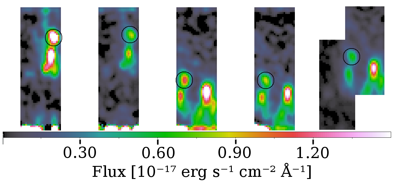
Figure 2: Colour-scale images in the four left panels show the plane with H$\alpha$ emission in the four single data cubes of the southern pointing of ESO111-G014. The black circles indicate the feature that was used to align the four data cubes. The right panel shows the plane with H$\alpha$ emission in the final, stacked data cube.

After stacking, cubes were reshaped such that both spatial dimensions have pixel sizes of 1 arcsec. For this task the scipy (Jones et al., 2001) function scipy.interpolate.griddata was used. Data were linearly interpolated to the new pixel size of $1\times 1$ arcsec.

Initially, observations of this WiFeS project do not include any world coordinate system (WCS) information in their file headers. To add this information in the file headers the following procedure was applied: right before the WiFeS observations were taken, an image with the acquisition and guiding (A&G) camera was taken. In the centre of this image the shadow of the WiFeS IFU is visible. We applied an astrometric solution to this A&G camera image using bright stars and the Aladin software (Bonnarel et al., 2000). Since the pixel size of the IFU cube (1 arcsec) and the location of the IFU within the A&G camera image (due to its shadow) are both known, we then simply transferred the astrometric solution from the A&G camera image to the IFU cubes. After this procedure, we measured the position of prominent features (e.g. peaks of star formation, stars) in collapsed maps of the WiFeS cubes and compared them to the positions of these features measured on the SuperCOSMOS $B_{j}$-band images. We find an average distance between the two position measurements of ($3\pm 6$) arcsec.

This procedure resulted in two data cubes for each pointing: one containing the red half of the spectrum and the other the blue half. To increase the signal-to-noise ratio of spectra, the spaxels in both cubes were binned such that one bin encompasses a star forming region and the H$\alpha$ and $\mathrm{N[II]}\,\lambda\,658.3\,\mathrm{nm}$ emission lines are visible in the resulting spectrum. These star forming regions were defined by hand on the H$\alpha$ emission planes of the WiFeS data cubes to be a connected region of H$\alpha$ emission (see Fig. 1).

In pointings towards the edges of stellar discs, the one-dimensional spectra of individual star forming regions do not pick up emission from the stellar continuum. In those cases the background was estimated as a constant from emission and sky line free parts of the spectrum (Wisnioski et al., 2015). For our data set we chose the following wavelength ranges: Indicating with $\lambda_{\alpha}$ and $\lambda_{N}$ the redshifted wavelengths of H$\alpha$ and $\mathrm{N[II]}\,\lambda\,658.3\,\mathrm{nm}$ lines, respectively, we chose the red window as [$\lambda_{N}$ + 2 nm, $\lambda_{N}$ + 7 nm] if $\lambda_{\alpha}<665$ nm, and [$\lambda_{\alpha}$ - 8 nm, $\lambda_{\alpha}$ - 3 nm] otherwise. The blue window is always [$\lambda_{\beta}$ - 8 nm, $\lambda_{\beta}$ - 3 nm], where $\lambda_{\beta}$ is the redshifted wavelength of the H$\beta$ line. We then took all the available data within these windows and calculated the 40th and 60th percentiles. The mean of the data in the 40th to 60th percentile range was then set as the constant background value for those spectra that do not show any stellar continuum.

If stellar continuum is detected in a spectrum of a star forming region, then the full spectrum (i.e. the blue and the red half) was used to fit a stellar population synthesis model and gas emission lines with the penalized pixel-fitting (pPXF) method and the python script by Cappellari & Emsellem (2004) and Cappellari (2017). pPXF used the stellar population synthesis models from the Vazdekis et al. (2010) library plus Gaussian emission lines. From the location of stellar absorption features, the stellar recession velocity in this star forming region was measured. pPXF provides the line strength for each modelled emission line (H$\alpha$, H$\beta$, $\mathrm{O[III]}\,\lambda\,500.7\,\mathrm{nm}$, and $\mathrm{N[II]}\,\lambda\,658.3\,\mathrm{nm}$). For the recession velocity of the gas it was assumed that there is only one kinematic component, and the recession velocity was modelled from all four emission lines simultaneously (i.e. one recession velocity measurement from the four emission lines).

The emission line fluxes were corrected for internal dust attenuation assuming the Calzetti et al. (2000) attenuation curve and $\rm R^{\prime}_{V}=4.05$ (see also Moran et al., 2012). From the corrected H$\alpha$, H$\beta$, $\mathrm{O[III]}\,\lambda\,500.7\,\mathrm{nm}$, and $\mathrm{N[II]}\,\lambda\,658.3\,\mathrm{nm}$ emission line fluxes, the gas-phase oxygen abundances were determined with the $O3N2$ and $N2$ method as described by Pettini & Pagel (2004).

We tested several options and found for spectra, in which the stellar continuum could be modelled with pPXF, that metallicity measurements based on the subtraction of a constant background and the $N2$ method agree with metallicities based on subtraction of a pPXF modelled stellar continuum and the $O3N2$ method. Hence, wherever possible we use $O3N2$ metallicities calculated from pPXF modelled emission line fluxes, otherwise the $N2$ method with the emission lines measured after subtraction of a constant background.

To de-project the on-sky galactocentric radius $r$, first the angle $\theta$ between the galaxy semi-major axis and the line between galaxy centre and star forming region was determined. The de-projected radius $r_{dpj}$ was then set to

$$r_{\rm dpj}=\frac{r\times\sqrt{(b\cos\theta)^{2}+(a\sin\theta)^{2}}}{b},$$ (1)

where $a$ and $b$ are the semi-major and semi-minor axis, respectively. Metallicity gradients were measured by fitting a line to the metallicities as a function of de-projected galactocentric radius. The slope of this line is the metallicity gradient.

Sample	Number of galaxies used here	relevant references	optical spectra	H i masses	metallicity indicator	min log M⋆ [M⊙]	max log M⋆ [M⊙]	Notes
(1)	(2)	(3)	(4)	(5)	(6)	(7)	(8)	(9)
hix	10	Lutz et al. (2017, 2018)	Y	Y	PP04 O3N2, N2	9.8	10.6
IC 4857	1	as hix	Y	Y	PP04 O3N2, N2	10.5		member of the original control sample
Hipass	1796	Dénes et al. (2014); Barnes et al. (2001); Meyer et al. (2004); Doyle et al. (2005)	N	Y	-	8.0	11.5	biased towards H i-rich objects, maximal redshift  0.04, parent sample for hix galaxies
SDSS MPA-JHU	60021	Abazajian et al. (2009); Salim et al. (2007)	Y	N	PP04 O3N2	8.0	11.5	to provide a benchmark mass-metallicity relation
GASS with longslit spectroscopy	96	Catinella et al. (2018); Moran et al. (2012)	Y	Y	PP04 O3N2	10.0	10.82	longslit spectra typically out to 1 Petrosian 90 % radius, see text for sample selection
CALIFA	227	Sánchez et al. (2014)	Y	N	PP04 O3N2	9.0	11.2	IFU data, the metallicity gradient is typically measured between 0.5 and 2 effective radii.

Table 3: Summary of the samples and data used in this paper. Column (1): name of the sample. Column (2): number of galaxies used in this paper. Column (3): references to the papers in which the sample and/or data are described in more detail. Column (4): whether (Y) or not (N) optical spectra are available for this sample. Column (5): whether (Y) or not (N) measurements of the H i mass are available for this sample. Column(6): which metallicity indicator was used to estimate the gas-phase metallicity. PP04 refers to Pettini & Pagel (2004). Columns (7) and (8): the minimum and maximum stellar mass limit of the sample, respectively. Column (9): Further notes.

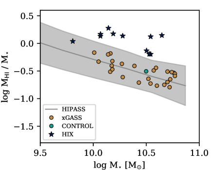
Figure 3: The H i gas mass fraction as a function of stellar mass for hix galaxies (blue stars), control galaxy IC 4857 (turquois circle), and those galaxies from GASS with an optical long-slit spectrum (yellow dots). The grey line is the running average of the Hipass parent sample and the grey shaded area the corresponding $1\,\sigma$ scatter.

2.4 Comparison samples

As only one of the original control galaxies was observed with WiFeS, data from the Sloan Digital Sky Survey (SDSS, York et al., 2000) data release 7 (Abazajian et al., 2009), and the (extended) GASS (Catinella et al., 2018, 2013, 2010; Moran et al., 2012) are used for comparison.

For the SDSS data, line emission and stellar mass measurements (Kauffmann et al., 2003; Salim et al., 2007) from the MPA-JHU SDSS DR7 catalogue are used. For galaxies within a redshift range of $0.002<z<0.06$ central metallicities were calculated from $5\,\sigma$ detected emission lines using again the $O3N2$ method. These data are used as a benchmark mass–metallicity relation in Sect. 3.2.

We also include data from the optical follow-up of GASS galaxies. These data are based on long-slit spectra rather than IFU spectra, and they cover radii to 1 Petrosian 90 % radius. The GASS survey measured the integrated atomic gas content of $\sim 1200$, stellar-mass selected galaxies. In addition, for about 200 galaxies optical long-slit spectra were obtained. From these spectra metallicity gradients were measured (Moran et al., 2012). Below, metallicity gradients, stellar masses, and H i mass fractions of star forming galaxies (i.e. near-UV-r colour bluer than 4.3) are used for comparison. To mimic the previous control sample, we restricted the sample to galaxies which are within $\pm 0.7\,\sigma$ of the Hipass running average in the H i mass fraction versus stellar mass plane (see Fig. 3). These GASS galaxies are shown as yellow dots in Fig. 3).

3 Results

3.1 Comparison of stellar, H$\alpha$ and H I velocities

Figure 4: Comparison of the recession velocities of different galaxy components: stars, H i, and ionised gas. Every panel compares two components. To account for the different redshifts of the different galaxies, the systemic velocity of the respective galaxy (see Table 1) was subtracted from the recession velocity measurement. No clear sign of counter rotation is visible.

To compare the kinematics of stars, and ionised and atomic gas, we consider their recession velocities minus the systemic velocity measured from the titled ring models in Lutz et al. (2018). A pairwise comparison of the three components is shown in Fig. 4. This figure shows for every spaxel how the local velocity of H i compares to that of the stars (left panel), to that of the H$\alpha$ line (middle panel), and the velocities of stars to the H$\alpha$ line (right panel). The horizontal and vertical lines indicate $\pm 100$ $\rm km\,s^{-1}$ of the systemic velocity, which is the velocity resolution of the used setup of the WiFeS spectrograph. Spaxels that are located in the upper left or lower right corner of this figure (red-shaded area) would indicate approaching movement in one component and receding movement in the other and thus counter-rotation. As can been seen, hardly any spaxels are located in the red regions. If the sign of the velocities of two components is different, this is usually within 100 $\rm km\,s^{-1}$, which is likely due to the low velocity resolution of the optical observations. Detailed kinematic maps for every galaxy can be found in Appendix A.

3.2 HIX galaxies on the mass–metallicity relation

Figure 5 shows the mass–metallicity relation for the hix and control galaxies that were observed with WiFeS. As mentioned above, the scatter of the mass–metallicity relation is driven by the H i content of the galaxies, where more H i-rich galaxies are more metal-poor at a given stellar mass (Bothwell et al., 2013; Brown et al., 2018). In Fig. 5, the black contours enclose 64% and 90 % of the full SDSS DR7 sample (as described in Sec. 2.4). The data points showing the hix galaxies (stars) and the control galaxy (large circle) are colour-coded according to H i mass fraction. For these galaxies, we only consider the most central metallicity measurement, which does not show line-ratios that are consistent with active galactic nuclei (AGN) emission.

There are no central WiFeS pointing (closer than $\approx 11$ kpc to the centre) available for ESO417-G018. Due to a metallicity gradient, ESO417-G018 is therefore located below the SDSS 90 % contour. The hix galaxies with the lowest central metallicity is, however, ESO290-G035. Apart from these two galaxies and ESO208-G026 (hix galaxy with lowest stellar mass), hix galaxies are generally located in the lower half of the SDSS scatter (black dotted lines). To sum it up, hix galaxies are generally expected to have lower metallicities in the centres, and indeed we find them to be predominantly located in the low metallicity half of the SDSS scatter.

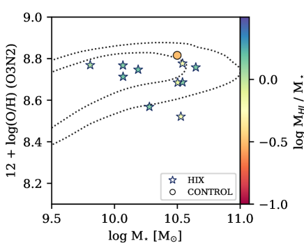
Figure 5: Mass–metallicity relation for the hix galaxies: we show the gas-phase metallicity (determined with the O3N2 parameter following Pettini & Pagel 2004) as a function of stellar mass. The contours enclose 64% and 90 % of SDSS galaxies. The circle indicates the control galaxy IC 4857 and hix galaxies are marked with stars. All symbols are also colour-coded by the H i mass fraction.

3.3 Gas-phase metallicity distribution

Exploiting the spatial information from the IFU spectral data, we extracted radial metallicity profiles and measured metallicity gradients. For a consistent comparison between our samples and the literature, the metallicity gradients are measured in units of dex kpc^-1. Metallicity gradients as a function of stellar mass are shown in Fig. 6 and data points are colour-coded by H i mass fraction. The grey line is the average Sánchez et al. (2014) gradient based on CALIFA data and the grey shaded area their $1\,\sigma$ scatter, within which all hix galaxies are located. Hence, hix galaxies do not show steeper metallicity profiles than average local spiral galaxies. In fact, they tend to be located at the flat end of the Sánchez et al. (2014) scatter and their average metallicity gradient is ($-0.016\pm 0.009$) dex kpc^-1. This means that the average Sánchez et al. (2014) gradient does not agree with the average hix gradient and its 1 $\sigma$ scatter, but they do agree within both their errors.

More recent work on metallicity gradients with SAMI and MaNGA galaxies generally agrees with Sánchez et al. (2014), despite detecting anti-correlations between metallicity gradients and stellar masses at low stellar masses (log M_⋆ [M_⊙] ¡ 9.6) (Poetrodjojo et al., 2018; Belfiore et al., 2017). We note, however, that diffuse emission significantly affects metallicity measurements in IFS data with poor spectral resolution, such as SAMI and MaNGA (Poetrodjojo et al., 2019). Furthermore, these surveys preferentially (only) report quantitative gradients in units of dex per effective radius or per isophotal radius. We thus refrain from more detailed comparison.

The control galaxy IC 4857 and the galaxies from the GASS Moran et al. (2012) sample are also mostly located within the $1\,\sigma$ scatter of CALIFA (circles in Fig. 6). We do not see the variation with stellar mass that was reported by Moran et al. (2012), perhaps because we only look at a small subsample. For the GASS galaxies we find an average metallicity gradient of ($-0.01\pm 0.01$) dex kpc^-1, which is consistent with the the average hix gradient, but again smaller than the average CALIFA gradient.

Figure 6: Metallicity gradient in dex kpc^-1 as a function of stellar mass. The grey line indicates the average gradient by Sánchez et al. (2014) and the grey shaded area the $1\,\sigma$ scatter. Stars indicate the metallicity gradient measured in hix galaxies, and the circles the gradients of the control galaxies (IC 4857 and GASS). All symbols are colour-coded by the H i mass fraction of the galaxy. Overall, hix and control galaxies behave similarly to the galaxies in the Sánchez et al. (2014) sample.

Moran et al. (2012) furthermore suggested that large, abrupt drops (of about 0.25 dex) in metallicity at the outskirts of the optical disc in massive galaxies can be caused by the inflow and distribution of pristine gas from the outskirts throughout the entire galaxy disc. Similarly, Sánchez Almeida et al. (2014b) found in a sample of dwarf galaxies, star forming regions with very low metallicities compared to other star forming regions within the same dwarf galaxy. They and Ceverino et al. (2016) argue that these metal-poor star forming regions are induced by pristine gas accretion. There are neither metallicity drops at the outskirts nor particularly metal-poor star forming regions observed in the hix and galaxies or in IC 4857 (for the detailed data see Appendix A).

4 Discussion and conclusion: optical spectra of HIX galaxies

We have presented the analysis of optical spectra of ten hix galaxies as well as a set of control galaxies. In a first step, measurements of the H$\alpha$, stellar (where available) and H i recession velocities in the hix galaxies and IC 4857 have been compared. Generally, the kinematics of all three components are similar. While the detection of counter-rotation, in particular between the stellar and gaseous components, would be strong evidence of recent accretion of large amounts of gas (Corsini, 2014), the opposite (no counter-rotation means no accretion) is not necessarily true. Hence, from the kinematics point of view, the evidence for recent accretion of large amounts of gas in hix galaxies is still inconclusive.

Using strong emission lines, gas-phase metallicities have been measured throughout the detected stellar discs of hix, control, and GASS galaxies. These measurements have been used to place these galaxies on the mass–metallicity relation and to compare their metallicity gradients, amongst each other and to the average of Sánchez et al. (2014).

On the mass–metallicity relation, most hix galaxies are located below the ridge of the relation. This is expected from and consistent with previous studies that found that H i-rich galaxies are generally metal poor (e.g. Bothwell et al. 2013; Hughes et al. 2013; Lagos et al. 2016; Brown et al. 2018). These studies, based on observations and on simulations, suggest that galaxies accrete gas stochastically, and that galaxies below the ridge of the mass–metallicity relation have recently accreted gas, which increased their gas content and decreased their gas-phase metallicity.

The radial distribution of the gas-phase metallicity (within the stellar disc) of hix galaxies appears similar to the one of galaxies with average H i contents. All measured gradients in hix galaxies are negative, i.e. they are more metal poor in the outskirts than in the centres, which is in agreement with the scenario where no major merger occurred recently. We have furthermore compared the hix metallicity gradients to the metallicity gradients of galaxies with less massive H i discs (drawn from the control sample and GASS). Regardless of their overall H i content, there is no significant difference in the metallicity gradients of these galaxies. We note again that all hix galaxies except ESO055-G013 have flatter gradients than the average Sánchez et al. (2014) gradient, yet all hix galaxies are within their 1$\sigma$ scatter. However, in the future we expect larger surveys, such as MaNGA or SAMI paired with dedicated H i observations to find an answer to this question.

The chemical evolution model of Ho et al. (2015) and Kudritzki et al. (2015) is able to reproduce measured metallicity gradients. This model suggests that the local metallicity is mostly dependent on the local stellar to total (H i + H₂) gas mass ratio. This has been observationally confirmed by Barrera-Ballesteros et al. (2018). At the galactocentric radii where gas-phase metallicities can be measured, both the H i and the stellar mass column densities in hix galaxies are similar to those of control galaxies. It is only at larger radii, that the H i column densities in control galaxies (or generally less H i-rich galaxies) are smaller than in hix galaxies, simply because the hix H i discs extend much further out. The stellar surface densities on the other hand are similar at all radii in hix and the comparison galaxies (similar stellar effective radii; Lutz et al., 2018). This means that the pace of radial metallicity variation in hix and comparison galaxies should be the same, and this is indeed what we observe. What is not observed in hix galaxies are large drops in metallicity or star forming regions with a very low metallicity compared to their surroundings. Thus, major accretion events are not likely (Moran et al., 2012; Sánchez Almeida et al., 2014a)

The analysis presented in previous papers (Lutz et al., 2018, 2017) suggests that hix galaxies are H i-rich because they are able to stabilise their H i disc against star formation due to a higher baryonic specific angular momentum. Examining the dark matter halo spin and H i content of galaxies simulated with a semi-analytic model, further showed that galaxies with a large H i disc tend to reside in dark matter halos with a large spin (i.e. angular momentum).

Based on the general interpretation of the scatter of the mass–metallicity relation, the new results presented here would suggest that despite the high baryonic specific angular momentum, metal-poor (accreted) gas would make its way from the outskirts to the centres of hix galaxies, where it dilutes the local gas. This would imply that hix galaxies are indeed those galaxies that recently accreted gas in a stochastic accretion process. However, this would also imply the following two points. First, their extreme H i mass would require them to accrete more gas than they contained before because they were selected to host at least 2.5 times more H i than expected from their optical properties. Second, the accreted gas must have a very high angular momentum and must increase the spin of the dark matter halo as well to comply with the findings from the semi-analytic models.

While Stewart et al. (2011) and Stewart et al. (2017) find in simulations that gas accreted in the cold mode would indeed come in with a high angular momentum and form a large co-rotating cold disc (at least in galaxies at redshift ¿ 1), the two points made above appear very extreme. Furthermore, Lara-López et al. (2013) find based on observations of H i content, specific star formation rate and metallicity that there are hardly any metal-poor, H i-rich galaxies at intermediate stellar mass and specific star formation rate. These are, however, exactly the characteristics of the hix galaxies.

One way to reconcile these findings is provided by the semi-analytic models of Boissier & Prantzos (2000). These models investigate the chemical evolution of galaxies with respect to the circular rotation velocity and the halo spin parameter. They find that galaxies residing in higher spin halos evolve more slowly than galaxies in lower spin halos. With a slower evolution comes less enrichment of the ISM and thus a lower gas-phase metallicity, much like the effect that makes metallicity gradients universal (Sánchez et al., 2014). These findings have been verified by SDSS observations (Cervantes-Sodi & Hernández, 2009). Catinella & Cortese (2015) propose a similar scenario for the most H i-rich galaxies detected at redshift 0.2.

Thus, the overall picture for the hix galaxies is the following: they reside in halos that have higher spins than the halos of average galaxies in terms of HI content, but not as high as necessary to host low surface brightness galaxies (Boissier et al., 2016, 2003; Kim & Lee, 2013). The high spin allows them to host larger H i discs than average. At the same time the high spin slows their evolution such that their ISM is (not yet) as enriched as it is in galaxies, which reside in average spin halos.

Appendix A Results for individual HIX galaxies

Figures 7 to 16 show detailed results for each of the hix galaxies individually. The maps of stellar and ionised gas kinematics, as well as the maps of metallicity (Panels (d), (e), and (g)), were obtained with the following procedure: for each star forming region (their borders are shown in Panel (b)) we derived one measurement of recession velocity or metallicity. We thus assign this measurement to the entire star forming region.

The rescaled profile in panel (i) was obtained in the following way. First the H i mass expected from the Dénes et al. (2014) relation was calculated. Then the expected H i radius (R_HI,exp, a 1 $\rm M_{\odot}\,pc^{-2}$ isophotal radius) was calculated from the relation by Wang et al. (2016). Then the radii of the profile were rescaled with a factor R_HI,exp / R_HI,mea , where R_HI,mea is the measured H i radius from Lutz et al. (2018).

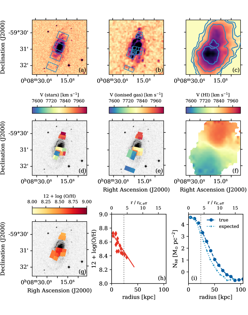
Figure 7: ESO111-G014: (a): Pointings are overlaid on SuperCOSMOS $B_{j}$-band images. (b): Star forming regions marked on a GALEX $FUV$ images (again $B_{j}$-band image for ESO208-G026). (c): H i moment 0 (intensity) map. Contours are at 0.5, 1.0, 2.5, 5.0, 7.5  $\rm M_{\odot}\,pc^{-2}$. (d): Stellar kinematics of single star forming regions overlaid on $B_{j}$-band image. (e): H$\alpha$ recession velocities of single star forming regions overlaid on $B_{j}$-band image. (f): H i moment 1 (velocity) map. (g): Metallicity measurements in single star forming regions overlaid on $B_{j}$-band image. (h): Radial profile of metallicities with linear fit to the profile, whose slope is the metallicity gradient. The grey dashed line marks the 25 mag arcsec^-2 isophotal radius. (i): Radial profile of H i column density. Dark blue circles and dashed line show the measured values corrected for inclination. Light blue points and dotted line show the profile rescaled to a 1 $\rm M_{\odot}\,pc^{-2}$ isophotal radius if the galaxy had average H i content (for more details see text). The grey dashed line again indicates the 25 mag arcsec^-2 isophotal radius. (a) to (g): All seven panels have the same spatial size; north is up and east is left. (d) to (e): Colour scale of the velocities is the same in all three panels.

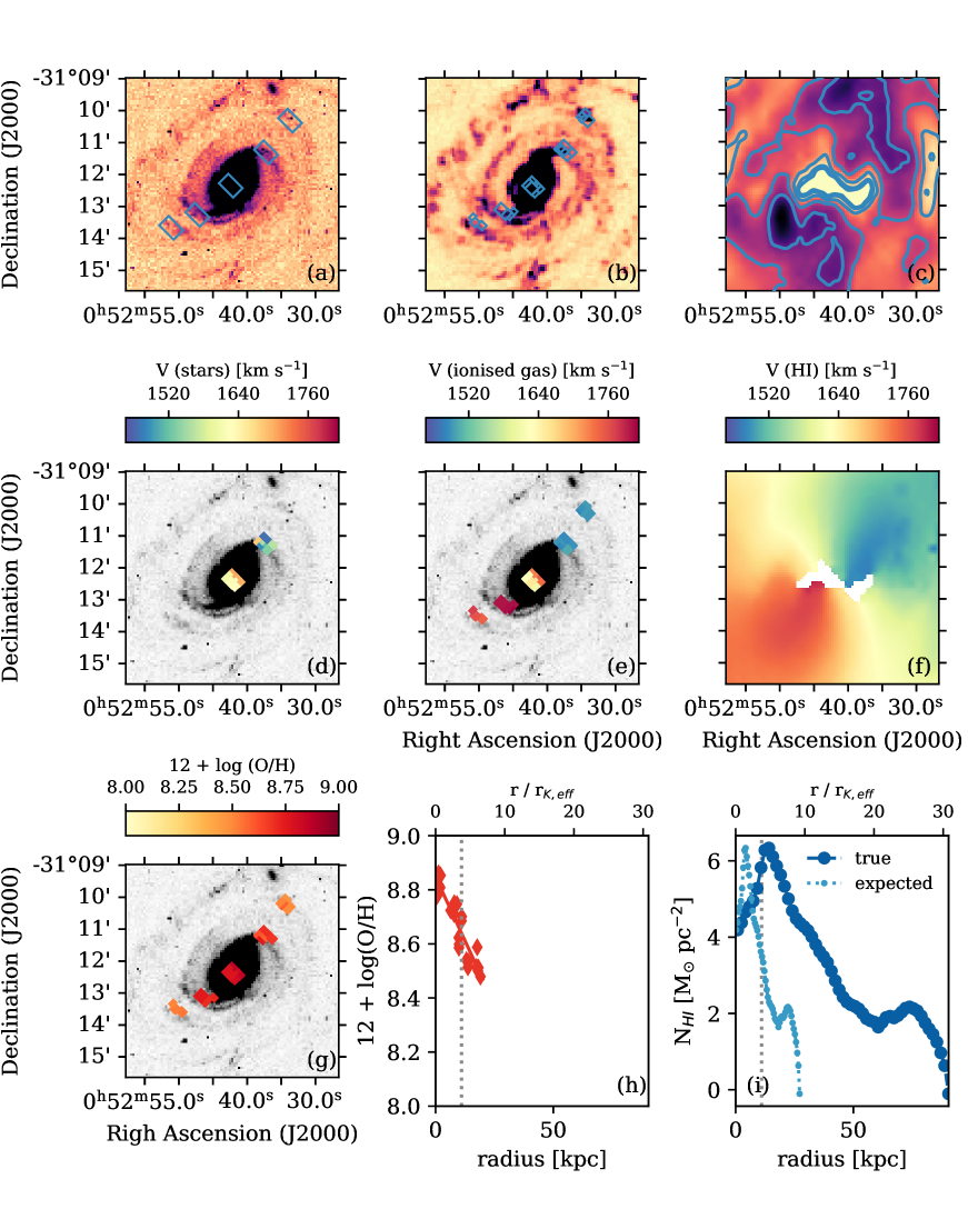
Figure 8: NGC289. Panels as in Fig. 7.

Figure 9: ESO245-G010. Panels as in Fig. 7.

Figure 10: ESO417-G018. Panels as in Fig. 7.

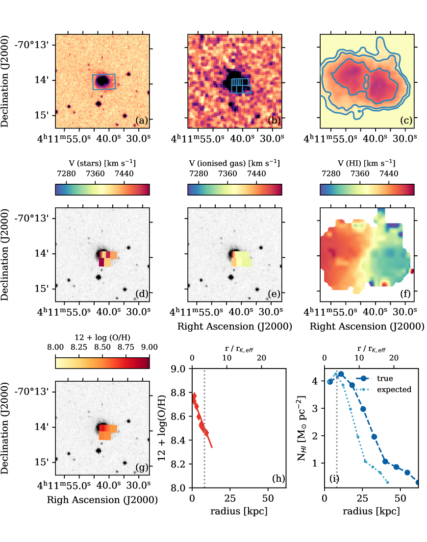
Figure 11: ESO055-G013. Panels as in Fig. 7.

Figure 12: ESO208-G026. Panels as in Fig. 7.

Figure 13: ESO378-G003. Panels as in Fig. 7.

Figure 14: ESO381-G005. Panels as in Fig. 7.

Figure 15: ESO075-G006. Panels as in Fig. 7.

Figure 16: ESO290-G035. Panels as in Fig. 7.

Appendix B Results for IC 4857

Figure 17 shows the detailed results of IC 4857, which is the only hix-control galaxy that was observed with WiFeS. Figure 17 shows the same data as Figs. 7 to 16.

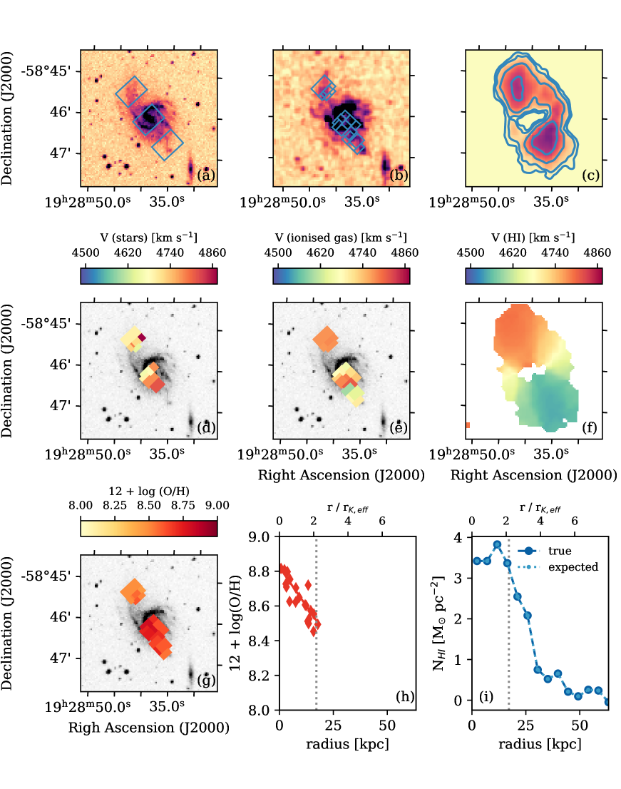
Figure 17: IC 4857. Panels as in Fig. 7.