Dissecting strong-field excitation dynamics with atomic-momentum spectroscopy

Abstract

Observation of internal quantum dynamics relies on correlations between the system being observed and the measurement apparatus. We propose using the center-of-mass (c.m.) degrees of freedom of atoms and molecules as a “built-in” monitoring device for observing their internal dynamics in non-perturbative laser fields. We illustrate the idea on the simplest model system - the hydrogen atom in an intense, tightly-focused infrared laser beam. To this end, we develop a numerically-tractable, quantum-mechanical treatment of correlations between internal and c.m. dynamics. We show that the transverse momentum records the time excited states experience the field, allowing femtosecond reconstruction of the strong-field excitation process. The ground state becomes weak-field seeking, an unambiguous and long sought-for signature of the Kramers-Henneberger regime.

The process of measurement in quantum mechanics relies on establishing a correlation between an internal quantum degree of freedom and a classical degree of freedom of a measurement apparatus. Finding a suitable classical outcome for a quantum system of interest is particularly important for achieving optimal temporal and spatial resolution. One classical degree of freedom available to every gas-phase system is the translational motion of its center of mass (c.m.), effectively attaching an individual measurement apparatus to each atom or molecule. The closely-related prescription of using the c.m. motion as a control device has been very successful in MössbauerN N Greenwood (1971) and other Doppler spectroscopiesKlaft et al. (1994).

The coupling between the internal quantum dynamics and the c.m. motion has not received much attention in strong-field atomic, molecular, and optical (AMO) science. In intense visible and infra-red fields, this coupling is a subtle effect, intimately connected to the breakdown of the dipole approximation. The fundamental importance of non-dipole effects have been recognized early onReiss (1990); Chirilă and Lein (2008); Reiss (2008), but only recently, enabled by refined theoretical and experimental approaches, processes beyond the dipole-approximation are coming into focus. These include radiation pressureLudwig et al. (2014), momentum distribution between fragments upon ionizationSmeenk et al. (2011); Chelkowski et al. (2014); Hartung et al. (2019), chiral effects in HHGCireasa et al. (2015), and atomic accelerationEichmann et al. (2009). These effects have been investigated for very intense (relativistic and near-relativistic) infra-red (IR) fieldsDammasch et al. (2001); Klaiber et al. (2013, 2017); Palaniyappan et al. (2005), as well as for shorter-wavelength fields which are becoming available in the strong-field regimeFørre and Simonsen (2014).

Because the c.m. coupling effects in strong-field physics are small, numerical treatment of their contribution is challenging. The standard technique appears to be the treatment on full-product gridsChelkowski et al. (2015), which would require a 6D numerical simulation even for the simplest realistic target – the hydrogen atom.

In this Letter we show that adding an artificial trapping potential, chosen not to disturb the c.m. motion, allows the effective dimensionality of the problem to be reduced to 3D. This enables detailed computational investigation of c.m. dynamics of strong-field processes. By using the c.m. motion as the “built-in” measurement apparatus, we obtain information on the dynamics of the excited-state formation in intense IR fields. Using this technique, we provide the first unambiguous, experimentally-realizable method for confirming the atomic ground state transiently entering the Kramers-Henneberger (KH) regime in such fields.

In the KH (or acceleration) frame of reference, the laser field dominates the electronic motion. For a laser field with the peak electric field amplitude $F_{0}$ and carrier frequency $\omega$, linearly polarized along the direction $\hat{n}$, the lowest-order Fourier component of the interaction potential in the KH frame takes the formHenneberger (1968):

$$U_{\rm KH}\!\left(\vec{r}\right) =\frac{1}{2\pi}\int_{0}^{2\pi}U\!\left(\vec{r}+\vec{l}_{0}\sin\!\left(\tau\right)\right)d\tau,$$ (1)

where $U$ is the interaction potential in the laboratory frame and the electron oscillation amplitude $\vec{l}_{0}=\hat{n}F_{0}\omega^{-2}$.

If higher-order corrections to Eq. (1) can be neglected for a given state, the system is said to be in the Kramers-Henneberger regime. A remarkable property of the KH states in low-frequency fields is that the effective polarizability rapidly approaches $-\omega^{-2}$Wei et al. (2017) with increasing $\vec{l}_{0}$ magnitude. As the result, a system in a KH state experiences the same ponderomotive potential as a free electron.

Kramers-Henneberger states have been postulated to explain photoelectron spectra in strong fieldsMorales et al. (2011), ionization-free filamentation in gasesRichter et al. (2013), and ponderomotive acceleration of neutral excited statesEichmann et al. (2009); Eilzer et al. (2014); Zimmermann and Eichmann (2016); Wei et al. (2017); Schulze et al. (2017); Zimmermann et al. (2018). Rydberg states readily satisfy the KH criteria in intense IR fields, and are commonly accepted to be in the KH regime in such fields. Because the KH states exist only transiently in the presence of the intense field, their unambiguous detection remains elusiveWei et al. (2017). The mechanism of their formation in low-frequency fields, and for the ground state even their existence, remain controversialPopov et al. (1999); Gavrila (2002); Popov et al. (2003); Simbotin et al. (2004); Gavrila et al. (2008), despite extensive investigationde Boer and Muller (1992); Jones et al. (1993); Nubbemeyer et al. (2008); Wolter et al. (2014); Piraux et al. (2017); Ortmann et al. (2018); Chen et al. (2012); Li et al. (2014); Zimmermann et al. (2017).

In the simplest case of a 1-electron, neutral atom, the laboratory-frame Hamiltonian is given by (unless noted otherwise, atomic units ($\hbar\!=\!m\!=\!|e|\!=\!1$) are used throughout):

$$\hat{H} =\frac{1}{2m_{1}}\left(\hat{p}_{1}+\vec{A}\!\left(\vec{r}_{1},t\right)\right)^{2}+\frac{1}{2m_{2}}\left(\hat{p}_{2}-\vec{A}\!\left(\vec{r}_{2},t\right)\right)^{2}$$

$$+v\!\left(\vec{\chi}\right)+u\!\left(\vec{R}\right)$$ (2)

where $\hat{p}_{1,2}$ are the momentum operators of particles $1$ (electron, charge $q_{1}\!\!=\!\!-1$) and $2$ (nucleus, $q_{2}\!\!=\!\!+1$), $\vec{A}\!\left(\vec{r},t\right)$ is the transverse ($\hat{\nabla}\cdot\vec{A}=0$) laboratory-space vector-potential, $v\!\left(\vec{\chi}\right)$ is the interaction potential between the particles, and $u\!\left(\vec{R}\right)$ is the c.m. trapping potential (in free space, $u\!=\!0$). Finally, $\vec{\chi}=\vec{r}_{1}-\vec{r}_{2}$ and $\vec{R}=(m_{1}/M)\vec{r}_{1}+(m_{2}/M)\vec{r}_{2}$, where $M\!=\!m_{1}+m_{2}$.

For systems of interest here, $m_{1}\!\ll\!m_{2}$. Introducing $\mu\!=\!m_{1}m_{2}/M$ and neglecting correction terms of the order $O\!\left(\mu/M\right)$ in the laser interaction, Eq. (2) simplifies toŠindelka et al. (2006):

$$\hat{H}_{\rm CoM} =\hat{H}_{\chi}+\hat{H}_{R}$$ (3)

$$\hat{H}_{\chi} =\frac{1}{2\mu}\left(\hat{p}_{\chi}+\vec{A}\!\left(\vec{R}+\vec{\chi},t\right)\right)^{2}+v\!\left(\vec{\chi}\right)$$ (4)

$$\hat{H}_{R} =\frac{1}{2M}\hat{p}_{R}^{2}+u\!\left(\vec{R}\right)\text{.}$$ (5)

We have verified that the terms omitted in Eq. (3) do not affect the results reported belowsup .

The appropriate choice of the trapping potential $u\!\left(\vec{R}\right)$ in Eq. (5) and the shape of the initial c.m. wavepacket are the key ingredients of our treatment. The extent of the c.m. wavepacket should be on the order of the thermal de Broglie wavelength of the target gas. The trapping potential should not significantly disturb the targeted observables on the time scale of the simulation. We have verified that the parabolic trapping potential used presently satisfies these requirementssup .

The general-case treatment of Eq. (3), which contains a non-separable coupling term through $\vec{A}\!\left(\vec{R}+\vec{\chi},t\right)$, remains a formidable numerical task. For the short (sub-picosecond) and moderately-intense IR fields, the c.m. displacements remain small compared to both the characteristic electron excursion and the laser-field wavelength. We therefore seek solutions of the time-dependent Schrödinger equation (TDSE) in the close-coupling form:

$$\Psi\!\left(\vec{\chi},\vec{R},t\right) =\sum_{n}\phi_{n}\!\left(\vec{\chi},t\right)\zeta_{n}\!\left(\vec{R}\right)$$ (6)

(From now on, we will omit arguments of $\phi_{n}$, $\zeta_{n}$ and other spatially- and time-dependent quantities, as long as their choice is unambiguous.) In Eq. (6), functions $\zeta_{n}$ are orthonormalized, time-independent eigenfunctions of $\hat{H}_{R}$ (Eq. (5)) with eigenvalues $\epsilon_{n}$. We assume that the potential $u\!\left(\vec{R}\right)$ in Eq. (5) is such that the set of the discrete solutions $\{\zeta_{n}\}$ is complete.

Substituting the Ansatz (6) into the TDSE for the Hamiltonian (3) and projecting on each $\zeta_{m}$ on the left, we obtain:

$$\mathrm{i}\frac{\partial}{\partial t}\phi_{m} =\left(\hat{h}+\epsilon_{m}\right)\phi_{m}+\sum_{n}\hat{h}_{mn}\phi_{n}.$$ (7)

The explicit form of the one-electron operators $\hat{h}$ and $\hat{h}_{mn}$ is given by the Eqs. (LABEL:eqn:tdse-h)–(LABEL:eqn:tdse-kappa)sup .

The system of coupled PDEs (7) can be propagated in time at a cost comparable to that of a standard, fixed-nuclei electronic TDSE, provided that the number of the nuclear-coordinate channels is not excessive. At the end of the pulse, the expectation of a c.m. observable $\hat{O}$, conditional on the internal degree of freedom being described by a normalized wavefunction $\phi_{a}\!\left(\chi\right)$, is given by:

$$\left<\hat{O}\right>_{a}= \sum_{mn}\left<\zeta_{m}|\hat{O}|\zeta_{n}\right>\left<\phi_{m}|\phi_{a}\right>\left<\phi_{a}|\phi_{n}\right>\text{.}$$ (8)

Choosing $\hat{O}=\hat{p}_{R}$ and $\hat{O}=\hat{1}$ yields the expectation of the momentum and the state population, respectively. The c.m. velocity of the atom in an internal state $\phi_{a}$ is then:

$$\mathrm{v}_{a}= \frac{1}{M}\frac{\left<\hat{p}_{R}\right>_{a}}{\left<\hat{1}\right>_{a}}\text{.}$$ (9)

We emphasize that the quantity $\mathrm{v}_{a}$ is determined from the expectation values calculated after the field vanishes. It does not depend on field gauge choice, and defines a physical observable.

We solve Eq. (7) for a 3-dimensional hydrogen atom ($\mu\!=\!1$, $M\!=\!1836$), initially in the $1s$ electronic ground state, exposed to a Gaussian pulse of beam waist $w_{0}=30236$ $a_{0}$, central frequency $\omega=0.057$ ($\lambda\approx 799$ nm), and full-width-half-maximum $\tau_{0}=220$ ($\approx 5.32$ fs). We choose for each Cartesian direction the following convention: $x$–beam propagation, $y$–transverse, and $z$–polarization. For further details of the numerical parameters seesup .

In a spatially non-uniform laser field, the excited atoms acquire the velocity both in the forward and in the transverse directions. The final c.m. velocity along laser polarization remains negligible, as required by symmetry. We have verified numerically that the forward velocity is insensitive to moderate spatial-intensity gradients. As a result, we discuss the two components of the velocity independently.

The forward (propagation-direction) component of velocity is a consequence of the radiation pressure. Strong-field excitation between hydrogenic levels with the principal quantum numbers $n$ and $n^{\prime}$ transfers the energy of $\Delta E=0.5(n^{-2}-n^{\prime-2})$ from the laser field to the atom. The corresponding momentum transfer is $\Delta E/c$, giving the forward velocity:

$$\Delta\mathrm{v}_{\rm f}= \frac{\Delta E}{Mc}\text{.}$$ (10)

Because it is determined solely by the initial and the final internal state of the atom, it contains no information on the intervening dynamics. Our numerical results (See Figs. LABEL:fig:beamcentre, LABEL:fig:w0halfsup ) are consistent with these expectations.

In the transverse direction the atoms are accelerated by the spatial gradient of the ponderomotive potential. Classically, the final outward velocity of an initially-stationary particle with dipole polarizability $\alpha$ entering the field at time $t_{b}$ in the vicinity of the beam waist ($x\!=\!0$, Eq. (LABEL:eqn:Az)) is given bysup :

$$\Delta\mathrm{v}_{\rm t}= \frac{\alpha}{4M}\int_{t_{b}}^{\infty}\frac{\partial}{\partial r}F_{0}^{2}\!\left(r,t\right)dt$$ (11)

where $F_{0}\!\left(r,t\right)$ is the envelope of the laser electric field (see Eq. (LABEL:eqn:F0)). The hydrogen ground state ($\alpha_{0}=4.5$) is expected to be accelerated towards stronger fields ($\frac{\partial}{\partial r}F_{0}^{2}<0$). Conversely, high-Rydberg states, which exhibit the free-electron-like dynamical polarizabilities in low-frequency fields ($\alpha_{\rm f}\!\approx\!-\omega^{-2}\approx-308$ at $799$ nm), are expected to move towards weaker fields.

A comparison of the calculated transverse velocity (Eq. (9)) with the classical Eq. (11) for a state a known polarizability allows us to infer $t_{b}$ — the time this state has entered the fieldsup . The integrand in Eq. (11) is negative, so that $t_{b}$ is a monotonic function of $\Delta\mathrm{v}_{\rm f}$ and defines a clock. Because $\alpha_{\rm f}$, the low-frequency dynamical polarizability of the Rydberg states, is a cycle-averaged quantitysup , the time resolution of this clock is $\approx 1/2$ of the laser-cycle duration ($\approx 1.3$ fs at 799 nm).

The composition of the Rydberg states populated by strong-field excitation is sensitively affected by channel closingsZimmermann et al. (2017); Piraux et al. (2017); Li et al. (2014). We therefore expect a similar effect to arise in the c.m. velocity spectroscopy. At $799$ nm, channel closings occur each $26$ TW cm^-2 ($\Delta I_{\rm channel}\!=\!4\omega^{3}$). For a tightly-focused beam used presently ($w_{0}=2\lambda$), in the vicinity of the beam half-waist a channel closing occurs each $648$ $a_{0}$, or $\approx\!34$ nm. We consider the channel-closing effects by repeating the calculations at seven, equidistant transverse points spaced by $216$ $a_{0}$, placed around the beam half-waist. We average the results equally among these points. This volume averaging effectively suppresses resonance contributions, which are highly sensitive to the intensity (See sup ).

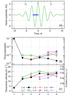
Figure 1: (Color online) Hydrogen atom initially at the half-waist position. The results are volume-averaged about the Cartesian point $(0,w_{0}/2\pm 648,0)$. The local peak intensity is $\approx\!607$ TW cm^-2. (a) Vector-potential at the initial position as a function of time. The upper horizontal axis gives the fraction of the pulse duration $\tau_{0}$. The blue dots on the time axis indicate the reconstructed excitation times, see Fig. 2 for details. (b) Population of the individual $m\!=\!0$ bound states after the end of the pulse. (c) Final c.m. velocity in the outward transverse direction in meters per second (1 atomic unit $\!\approx 2.19\!\times\!10^{6}$ m s^-1). The right vertical axis gives the time when a particle with $\alpha=\alpha_{f}$ needs to enter the field to reach the observed transverse velocity (Eq. (11)). The connecting lines in panels (b,c) are only a guide for the eye.

The maximum gradient of the ponderomotive potential occurs in the focal plane, $w_{0}/2$ away from the focal spot. We choose the point displaced in the $y$ direction, perpendicular to both the propagation and polarization directions. The volume-averaged numerical results at this point are illustrated in Fig. 1. The local peak intensity of the field is $\approx\!607$ TW cm^-2. The ionization is in the saturation regime, with $\approx\!9\%$ of the population surviving in the $1s$ ground state after the pulse. Additionally, $\approx\!2.4\%$ of the atoms are excited to Rydberg states with $n\!\leq\!6$. Although our simulation volume does not allow an accurate determination of excitation probabilities for higher Rydberg states, we estimate that at least $2\%$ of the atoms are left in Rydberg states with $n\!\geq\!7$. Most of the excited states possess magnetic quantum number $m\!=\!0$, same as the initial state.

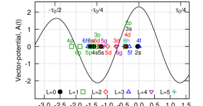
Figure 2: (Color online) Reconstructed excitation times (See text and Fig. 1 for the raw data). The vector potential at the Cartesian point $(0,w_{0}/2,0)$ is given by the black solid line. Peak of the envelope is at the time zero. Please note that the resolution of the envelope clock is $\approx 1/2$ laser cycle ($\approx 1.3$ fs).

For all electronic states in Fig. 1c other than the ground state, the final transverse velocities are in the range of $12$–$20$ m s^-1. Solving Eq. (11) for $t_{b}$ yields the excitation time. The results for the volume-averaged excitation time reconstruction are presented in Fig. 2. In all cases, excited states are formed within the laser cycle immediately preceeding the peak of the envelope. Although the excitation clock defined by the Eq. (11) does not offer true sub-cycle resolution, it appears that the Rydberg states with low principal quantum numbers tend to be populated later in the laser pulse. This observation is consistent with the expectations of the frustrated tunneling modelNubbemeyer et al. (2008): formation of the more compact, low-$n$ states requires a tunnel exit point closer to the nucleus and consequently higher electric field, reached closer to the peak of the envelope.

We present further fixed-intensity results (Figs. LABEL:fig:beamcentre–LABEL:fig:w0half:times), and explore the effects of the carrier-envelope phase (CEP, Figs. LABEL:fig:w0halfavepihalf, LABEL:fig:w0halfavepihalf:times), pulse duration (Figs. LABEL:fig:w0halfavelong, LABEL:fig:w0halfavelong:times), and non-paraxial effects arising in a tightly-focused beam (Figs. LABEL:fig:w0halfavepol, LABEL:fig:w0halfavepol:times) in sup . In all cases, we can successfully assign the preferred excitation times based on the volume-averaged c.m.-velocity spectra, confirming that the technique is universally applicable and experimentally realizable. With a few exceptions, the reconstructed excitation times are before the peak of the envelope, and tend to fall within the same laser cycle. For longer pulses (See Figs. LABEL:fig:w0halfavelong,LABEL:fig:w0halfavelong:times), the preferred excitation times shift to earlier times, before the peak of the envelope. They however remain clustered within one laser cycle.

Because the ponderomotive clock is not sub-cycle accurate, we cannot associate the time of the excitation with the specific phase of the field. It may be possible to improve the time resolution of the excitation clock using multi-color techniques, which have been successful for the reconstruction of the ionization and recollision times in high-harmonic spectroscopyShafir et al. (2012); Bruner et al. (2015). Another possibility involves breaking the symmetry of the interaction with a static, external magnetic field. Both possibilities are currently under investigation.

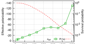
Figure 3: (Color online) Effective polarizability $\alpha_{\rm eff}$ (green solid line; left vertical axis) and survival probability (red dashed line; right vertical axis) of the $1s$ ground state. The spatio-temporal field profile is the same as in Fig. 1. The peak intensity $I_{0}$ varies from $50$ TW cm^-2 to $2$ PW cm^-2. The horizontal axis shows the local peak intensity at the initial, half-waist position of the atom ($I_{loc}\!\approx\!0.607\!\times\!I_{0}$).

One remarkable result seen in Fig. 1c, which so far has not been commented upon, is the behavior of the $1s$ ground state. For the laser pulse in Fig. 1a, it is weak-field seeking, reaching the final outward velocity of $\approx 3.2$ m s^-1. The low-field-seeking behavior of the $1s$ state persists for other field parameters as wellsup . The final $1s$ velocity is insensitive to channel-closing effects, indicating that it arises due to adiabatic modification of the ground state, rather than transient population of high-Rydberg states.

For the initial $1s$ state, $t_{b}\rightarrow-\infty$, and Eq. (11) yields the effective polarizability $\alpha_{\rm eff}$, shown as a function of the peak intensity of the laser pulse in Fig. 3. At intensities below $50$ TW cm^-2, the numerical accuracy is insufficient to determine the final c.m. velocity ( Fig. LABEL:fig:velocity-1s sup ). The effective polarizability is negative, as opposed to $+4.5$ expected for $1s$ in a weak field. It is characteristic of entering the Kramers-Henneberger regimeWei et al. (2017). Observation of Kramers-Henneberger regime for an atomic ground state in strong, low-frequency fields has been long sought after, with no unambiguous detection thus farWei et al. (2017).

To summarize, we have developed a computationally-tractable quantum mechanical approach to correlations between c.m. motion and internal electronic dynamics in strong, non-uniform laser fields. Using the technique, we demonstrate that the final c.m. velocity is sensitive to the internal excitation dynamics. In particular the transverse, ponderomotive velocity is determined by the total time the excited state spends in the field. In the absence of resonances, it yields a measurement of the preferential time of excitation. This procedure is robust to limited volume averaging, and can be applied for different CEP values, for longer pulses, and for non-paraxial beams. Finally, we demonstrate an unambiguous signature of the atomic ground state entering the Kramers-Henneberger regime in strong, low-frequency fields, which has been long sought-for. Taken together, our results suggest that c.m.-velocity spectroscopy is a powerful, and so far overlooked tool for understanding strong-field bound-state electronic dynamics on their natural timescale.

We expect that similar ideas, using a collective, nearly-classical degrees of freedom of a quantum system as an intrinsic measurement device may become useful in other contexts as well.

References

- N N Greenwood (1971) T C Gibb N N Greenwood, Mössbauer spectroscopy (Chapman and Hall (London), 1971).
- Klaft et al. (1994) I. Klaft, S. Borneis, T. Engel, B. Fricke, R. Grieser, G. Huber, T. Kühl, D. Marx, R. Neumann, S. Schröder, P. Seelig, and L. Völker, “Precision laser spectroscopy of the ground state hyperfine splitting of hydrogenlike ,” Phys. Rev. Lett. 73, 2425–2427 (1994).
- Reiss (1990) H. R. Reiss, “Complete Keldysh theory and its limiting cases,” Phys. Rev. A 42, 1476–1486 (1990).
- Chirilă and Lein (2008) C. C. Chirilă and M. Lein, “Effect of dressing on high-order harmonic generation in vibrating H2 molecules,” Phys. Rev. A 77, 043403 (2008).
- Reiss (2008) H. R. Reiss, “Limits on tunneling theories of strong-field ionization,” Phys. Rev. Lett. 101, 043002 (2008).
- Ludwig et al. (2014) A. Ludwig, J. Maurer, B. W. Mayer, C. R. Phillips, L. Gallmann, and U. Keller, “Breakdown of the dipole approximation in strong-field ionization,” Phys. Rev. Lett. 113, 243001 (2014).
- Smeenk et al. (2011) C. T. L. Smeenk, L. Arissian, B. Zhou, A. Mysyrowicz, D. M. Villeneuve, A. Staudte, and P. B. Corkum, “Partitioning of the linear photon momentum in multiphoton ionization,” Phys. Rev. Lett. 106, 193002 (2011).
- Chelkowski et al. (2014) Szczepan Chelkowski, André D. Bandrauk, and Paul B. Corkum, “Photon momentum sharing between an electron and an ion in photoionization: From one-photon (photoelectric effect) to multiphoton absorption,” Phys. Rev. Lett. 113, 263005 (2014).
- Hartung et al. (2019) A. Hartung, S. Eckart, S. Brennecke, J. Rist, D. Trabert, K. Fehre, M. Richter, H. Sann, S. Zeller, K. Henrichs, G. Kastirke, J. Hoehl, A. Kalinin, M. S. Schöffler, T. Jahnke, L. Ph H. Schmidt, M. Lein, M. Kunitski, and R. Dörner, “Magnetic fields alter strong-field ionization,” Nature Physics 15, 1222–1226 (2019).
- Cireasa et al. (2015) R. Cireasa, A. E. Boguslavskiy, B. Pons, M. C. H. Wong, D. Descamps, S. Petit, H. Ruf, N. Thire, A. Ferre, J. Suarez, J. Higuet, B. E. Schmidt, A. F. Alharbi, F. Legare, V. Blanchet, B. Fabre, S. Patchkovskii, O. Smirnova, Y. Mairesse, and V. R. Bhardwaj, “Probing molecular chirality on a sub-femtosecond timescale,” Nature Physics 11, 654 (2015).
- Eichmann et al. (2009) U. Eichmann, T. Nubbemeyer, H. Rottke, and W. Sandner, “Acceleration of neutral atoms in strong short-pulse laser fields,” Nature 461, 1261 (2009).
- Dammasch et al. (2001) Matthias Dammasch, Martin Dörr, Ulli Eichmann, Ernst Lenz, and Wolfgang Sandner, “Relativistic laser-field-drift suppression of nonsequential multiple ionization,” Phys. Rev. A 64, 061402 (2001).
- Klaiber et al. (2013) Michael Klaiber, Enderalp Yakaboylu, Heiko Bauke, Karen Z. Hatsagortsyan, and Christoph H. Keitel, “Under-the-barrier dynamics in laser-induced relativistic tunneling,” Phys. Rev. Lett. 110, 153004 (2013).
- Klaiber et al. (2017) M. Klaiber, K. Z. Hatsagortsyan, J. Wu, S. S. Luo, P. Grugan, and B. C. Walker, “Limits of strong field rescattering in the relativistic regime,” Phys. Rev. Lett. 118, 093001 (2017).
- Palaniyappan et al. (2005) S. Palaniyappan, A. DiChiara, E. Chowdhury, A. Falkowski, G. Ongadi, E. L. Huskins, and B. C. Walker, “Ultrastrong field ionization of Nen+ : Rescattering and the role of the magnetic field,” Phys. Rev. Lett. 94, 243003 (2005).
- Førre and Simonsen (2014) Morten Førre and Aleksander Skjerlie Simonsen, “Nondipole ionization dynamics in atoms induced by intense XUV laser fields,” Phys. Rev. A 90, 053411 (2014).
- Chelkowski et al. (2015) Szczepan Chelkowski, André D. Bandrauk, and Paul B. Corkum, “Photon-momentum transfer in multiphoton ionization and in time-resolved holography with photoelectrons,” Phys. Rev. A 92, 051401 (2015).
- Henneberger (1968) Walter C. Henneberger, “Perturbation method for atoms in intense light beams,” Phys. Rev. Lett. 21, 838–841 (1968).
- Wei et al. (2017) Qi Wei, Pingxiao Wang, Sabre Kais, and Dudley Herschbach, “Pursuit of the Kramers-Henneberger atom,” Chem. Phys. Lett. 683, 240 – 246 (2017).
- Morales et al. (2011) Felipe Morales, Maria Richter, Serguei Patchkovskii, and Olga Smirnova, “Imaging the Kramers-Henneberger atom,” Proc. Natl. Acad. Sci. USA 108, 16906–16911 (2011).
- Richter et al. (2013) Maria Richter, Serguei Patchkovskii, Felipe Morales, Olga Smirnova, and Misha Ivanov, “The role of the kramers–henneberger atom in the higher-order kerr effect,” New Journal of Physics 15, 083012 (2013).
- Eilzer et al. (2014) S. Eilzer, H. Zimmermann, and U. Eichmann, “Strong-field Kapitza-Dirac scattering of neutral atoms,” Phys. Rev. Lett. 112, 113001 (2014).
- Zimmermann and Eichmann (2016) H Zimmermann and U Eichmann, “Atomic excitation and acceleration in strong laser fields,” Physica Scripta 91, 104002 (2016).
- Schulze et al. (2017) D. Schulze, A. Thakur, A.S. Moskalenko, and J. Berakdar, “Accelerating, guiding, and sub-wavelength trapping of neutral atoms with tailored optical vortices,” Ann. Phys. 529, 1600379 (2017).
- Zimmermann et al. (2018) H. Zimmermann, S. Meise, A. Khujakulov, A. Magaña, A. Saenz, and U. Eichmann, “Limit on excitation and stabilization of atoms in intense optical laser fields,” Phys. Rev. Lett. 120, 123202 (2018).
- Popov et al. (1999) AM Popov, OV Tikhonova, and EA Volkova, “Applicability of the Kramers-Henneberger approximation in the theory of strong-field ionization,” J. Phys. B 32, 3331–3345 (1999).
- Gavrila (2002) M Gavrila, “Atomic stabilization in superintense laser fields,” J. Phys. B 35, R147–R193 (2002).
- Popov et al. (2003) AM Popov, OV Tikhonova, and EA Volkova, “Strong-field atomic stabilization: numerical simulation and analytical modelling,” J. Phys. B 36, R125–R165 (2003).
- Simbotin et al. (2004) I Simbotin, M Stroe, and M Gavrila, “Quasistationary stabilization and atomic dichotomy in superintense low-frequency fields,” Laser Phys. 14, 482–491 (2004).
- Gavrila et al. (2008) M. Gavrila, I. Simbotin, and M. Stroe, “Low-frequency atomic stabilization and dichotomy in superintense laser fields from the high-intensity high-frequency Floquet theory,” Phys. Rev. A 78, 033404 (2008).
- de Boer and Muller (1992) M. P. de Boer and H. G. Muller, “Observation of large populations in excited states after short-pulse multiphoton ionization,” Phys. Rev. Lett. 68, 2747–2750 (1992).
- Jones et al. (1993) R. R. Jones, D. W. Schumacher, and P. H. Bucksbaum, “Population trapping in Kr and Xe in intense laser fields,” Phys. Rev. A 47, R49–R52 (1993).
- Nubbemeyer et al. (2008) T. Nubbemeyer, K. Gorling, A. Saenz, U. Eichmann, and W. Sandner, “Strong-field tunneling without ionization,” Phys. Rev. Lett. 101, 233001 (2008).
- Wolter et al. (2014) Benjamin Wolter, Christoph Lemell, Matthias Baudisch, Michael G. Pullen, Xiao-Min Tong, Michaël Hemmer, Arne Senftleben, Claus Dieter Schröter, Joachim Ullrich, Robert Moshammer, Jens Biegert, and Joachim Burgdörfer, “Formation of very-low-energy states crossing the ionization threshold of argon atoms in strong mid-infrared fields,” Phys. Rev. A 90, 063424 (2014).
- Piraux et al. (2017) B. Piraux, F. Mota-Furtado, P. F. O’Mahony, A. Galstyan, and Yu. V. Popov, “Excitation of Rydberg wave packets in the tunneling regime,” Phys. Rev. A 96, 043403 (2017).
- Ortmann et al. (2018) L. Ortmann, C. Hofmann, and A. S. Landsman, “Dependence of Rydberg-state creation by strong-field ionization on laser intensity,” Phys. Rev. A 98, 033415 (2018).
- Chen et al. (2012) Shaohao Chen, Xiang Gao, Jiaming Li, Andreas Becker, and Agnieszka Jaroń-Becker, “Application of a numerical-basis-state method to strong-field excitation and ionization of hydrogen atoms,” Phys. Rev. A 86, 013410 (2012).
- Li et al. (2014) Qianguang Li, Xiao-Min Tong, Toru Morishita, Hui Wei, and C. D. Lin, “Fine structures in the intensity dependence of excitation and ionization probabilities of hydrogen atoms in intense 800-nm laser pulses,” Phys. Rev. A 89, 023421 (2014).
- Zimmermann et al. (2017) H. Zimmermann, S. Patchkovskii, M. Ivanov, and U. Eichmann, “Unified time and frequency picture of ultrafast atomic excitation in strong laser fields,” Phys. Rev. Lett. 118, 013003 (2017).
- Šindelka et al. (2006) Milan Šindelka, Nimrod Moiseyev, and Lorenz S. Cederbaum, “Dipole and quadrupole forces exerted on atoms in laser fields: The nonperturbative approach,” Phys. Rev. A 74, 053420 (2006).
- (41) See Supplemental Material [URL to be inserted by publisher] for computational details, supplemental derivations, and additional results, which includes Refs. Manolopoulos (2002); Lax et al. (1975); Patchkovskii and Muller (2016).
- Shafir et al. (2012) Dror Shafir, Hadas Soifer, Barry D. Bruner, Michal Dagan, Yann Mairesse, Serguei Patchkovskii, Misha Yu. Ivanov, Olga Smirnova, and Nirit Dudovich, “Resolving the time when an electron exits a tunnelling barrier,” Nature 485, 343–346 (2012).
- Bruner et al. (2015) Barry D. Bruner, Hadas Soifer, Dror Shafir, Valeria Serbinenko, Olga Smirnova, and Nirit Dudovich, “Multidimensional high harmonic spectroscopy,” J. Phys. B 48, 174006 (2015).
- Manolopoulos (2002) David E. Manolopoulos, “Derivation and reflection properties of a transmission-free absorbing potential,” J. Chem. Phys. 117, 9552–9559 (2002).
- Lax et al. (1975) Melvin Lax, William H. Louisell, and William B. McKnight, “From Maxwell to paraxial wave optics,” Phys. Rev. A 11, 1365–1370 (1975).
- Patchkovskii and Muller (2016) Serguei Patchkovskii and H. G. Muller, “Simple, accurate, and efficient implementation of 1-electron atomic time-dependent Schrodinger equation in spherical coordinates,” Comp. Phys. Comm. 199, 153–169 (2016).