Convergence rates of the Semi-Discrete method for stochastic differential equations

Abstract.

We study the convergence rates of the semi-discrete (SD) method originally proposed in Halidias (2012), Semi-discrete approximations for stochastic differential equations and applications, International Journal of Computer Mathematics, 89(6). The SD numerical method was originally designed mainly to reproduce qualitative properties of nonlinear stochastic differential equations (SDEs). The strong convergence property of the SD method has been proved, but except for certain classes of SDEs, the order of the method was not studied. We study the order of ${\mathcal{L}}^{2}$-convergence and show that it can be arbitrarily close to $1/2.$ The theoretical findings are supported by numerical experiments.

1. Introduction

We are interested in the following class of scalar stochastic differential equations (SDEs),

(1) $$dx_{t}=a(t,x_{t})dt+b(t,x_{t})dW_{t},\qquad t\in[0,T],$$

where $a,b:[0,T]\times{\mathbb{R}}\rightarrow{\mathbb{R}}$ are measurable functions such that (1) has a unique solution and $x_{0}$ is independent of all $\{W_{t}\}_{t\geq 0}.$ SDE (1) has non-autonomous coefficients, i.e. $a(t,x),b(t,x)$ depend explicitly on $t.$ SDEs of the type (1), apart from certain cases, c.f [1], do not have explicit solutions. Therefore the need for numerical approximations for simulations of the paths $x_{t}(\omega)$ is apparent. We are interested in strong approximations (mean-square) of (1), in the case of nonlinear drift and diffusion coefficients. In the same time we want to reproduce some qualitative properties of the solution process such as domain preservation.

In this direction, we study the semi-discrete (SD) method originally proposed in [2] and further investigated in [3], [4], [5], [6], [7] and recently in [8] and [9]. The main idea behind the semi-discrete method is freezing on each subinterval appropriate parts of the drift and diffusion coefficients of the solution at the beginning of the subinterval so as to obtain explicitly solved SDEs. Of course the way of freezing (discretization) is not unique.

The SD method is a fixed-time step explicit numerical method which strongly converges to the exact solution and also preserves the domain of the solution; if for instance the solution process $x_{t}$ is nonnegative then the approximation process $y_{t}$ is also nonnegative.

Our main goal is to establish the ${\mathcal{L}}^{2}$-convergence of the SD method and show that it can be arbitrarily close to $1/2.$

Explicit fixed-step Euler methods fail to strongly converge to solutions of (1) when the drift or diffusion coefficient grows superlinearly [10, Theorem 1]. Tamed Euler methods were proposed to overcome the aforementioned problem, cf. [11, (4)], [12, (3.1)], [13] and references therein; nevertheless in general they fail to preserve positivity. We also mention the method presented in [14] where they use the Lamperti-type transformation to remove the nonlinearity from the diffusion to the drift part of the SDE. Moreover, adaptive time-stepping strategies applied to explicit Euler method are an alternative way to address the problem and there is an ongoing research on that approach, see [15], [16] and [17]. Our approach is motivated by the truncated Euler-Maruyama method, see [18], [19]. At this point, we would like to refer to a different approach in solving stochastic differential equations where the main idea is to reduce, even eliminate in cases, the systematic error that appears in the computation of the mean value of a function of the solution of the SDE, c.f. the recent work [20] or [21].

The outline of the article is the following. In Section 2 we present the setting and the assumptions, Section 3 includes among other results our main result, that is Theorem 2, with their proofs. Section 4 provides a numerical illustration and Section 5 concluding remarks.

2. Setting and Assumptions

Throughout, let $T>0$ and $(\Omega,{\mathcal{F}},\{{\mathcal{F}}_{t}\}_{0\leq t\leq T},{\mathbb{P}})$ be a complete probability space, meaning that the filtration $\{{\mathcal{F}}_{t}\}_{0\leq t\leq T}$ satisfies the usual conditions, i.e. is right continuous and ${\mathcal{F}}_{0}$ includes all ${\mathbb{P}}$-null sets. Let $W_{t,\omega}:[0,T]\times\Omega\rightarrow{\mathbb{R}}$ be a one-dimensional Wiener process adapted to the filtration $\{{\mathcal{F}}_{t}\}_{0\leq t\leq T}.$ Consider SDE (1), which we rewrite here in its integral form

(2) $$x_{t}=x_{0}+\int_{0}^{t}a(s,x_{s})ds+\int_{0}^{t}b(s,x_{s})dW_{s},\quad t\in[0,T],$$

which admits a unique strong solution. In particular, we assume the existence of a predictable stochastic process $x:[0,T]\times\Omega\rightarrow{\mathbb{R}}$ such that ([22, Def. 2.1]),

$$\{a(t,x_{t})\}\in{\mathcal{L}}^{1}([0,T];{\mathbb{R}}),\quad\{b(t,x_{t})\}\in{\mathcal{L}}^{2}([0,T];{\mathbb{R}})$$

and

$${\mathbb{P}}\left[x_{t}=x_{0}+\int_{0}^{t}a(s,x_{s})ds+\int_{0}^{t}b(s,x_{s})dW_{s}\right]=1,\quad\hbox{ for every }t\in[0,T].$$

Assumption 1.

Let $f(s,r,x,y),g(s,r,x,y):[0,T]^{2}\times{\mathbb{R}}^{2}\rightarrow{\mathbb{R}}$ be such that $f(s,s,x,x)=a(s,x),g(s,s,x,x)=b(s,x),$ where $f,g$ satisfy the following condition $(\phi\equiv f,g)$

$$|\phi(s_{1},r_{1},x_{1},y_{1})-\phi(s_{2},r_{2},x_{2},y_{2})|\leq C_{R}\Big{(}|s_{1}-s_{2}|+|r_{1}-r_{2}|+|x_{1}-x_{2}|+|y_{1}-y_{2}|\Big{)}$$

for any $R>0$ such that $|x_{1}|\vee|x_{2}|\vee|y_{1}|\vee|y_{2}|\leq R,$ where the quantity $C_{R}$ depends on $R$ and $x\vee y$ denotes the maximum of $x,y.$

Let us now recall the SD scheme. Consider the equidistant partition $0=t_{0}<t_{1}<...<t_{N}=T$ and $\Delta=T/N.$ We assume that for every $n\leq N-1,$ the following SDE

(3) $$y_{t}=y_{t_{n}}+\int_{t_{n}}^{t}f(t_{n},s,y_{t_{n}},y_{s})ds+\int_{t_{n}}^{t}g(t_{n},s,y_{t_{n}},y_{s})dW_{s},\quad t\in(t_{n},t_{n+1}],$$

with $y_{0}=x_{0}$ a.s., has a unique strong solution.

In order to compare with the exact solution $x_{t},$ which is a continuous time process, we consider the following interpolation process of the semi-discrete approximation, in a compact form,

(4) $$y_{t}=y_{0}+\int_{0}^{t}f(\hat{s},s,y_{\hat{s}},y_{s})ds+\int_{0}^{t}g(\hat{s},s,y_{\hat{s}},y_{s})dW_{s},$$

where $\hat{s}=t_{n}$ when $s\in[t_{n},t_{n+1}).$ Process (4) has jumps at nodes $t_{n}.$ The first and third variable in $f,g$ denote the discretized part of the original SDE. We observe from (4) that in order to solve for $y_{t}$, we have to solve an SDE and not an algebraic equation, thus in this context, we cannot reproduce implicit schemes, but we can reproduce the Euler scheme if we choose $f(s,r,x,y)=a(s,x)$ and $g(s,r,x,y)=b(s,x).$

In the case of superlinear coefficients the numerical scheme (4) converges to the true solution $x_{t}$ of SDE (2) and this is stated in the following, cf. [3],

Theorem 1 (Strong convergence).

Suppose Assumption 1 holds and (3) has a unique strong solution for every $n\leq N-1,$ where $x_{0}\in{\mathcal{L}}^{p}(\Omega,{\mathbb{R}}).$ Let also

$${\mathbb{E}}(\sup_{0\leq t\leq T}|x_{t}|^{p})\vee{\mathbb{E}}(\sup_{0\leq t\leq T}|y_{t}|^{p})<A,$$

for some $p>2$ and $A>0.$ Then the semi-discrete numerical scheme (4) converges to the true solution of (2) in the ${\mathcal{L}}^{2}$-sense, that is

(5) $$\lim_{\Delta\rightarrow 0}{\mathbb{E}}\sup_{0\leq t\leq T}|y_{t}-x_{t}|^{2}=0.$$

Relation (5) does not reveal the order of convergence. We choose a strictly increasing function $\mu:{\mathbb{R}}_{+}\rightarrow{\mathbb{R}}_{+}$ such that for every $s,r\leq T$

(6) $$\sup_{|x|\leq u}\left(|f(s,r,x,y)|\vee|g(s,r,x,y)|\right)\leq\mu(u)(1+|y|),\qquad u\geq 1.$$

The inverse function of $\mu,$ denoted by $\mu^{-1},$ maps $[\mu(1),\infty)$ to ${\mathbb{R}}_{+}.$ Moreover, we choose a strictly decreasing function $h:(0,1]\rightarrow[\mu(1),\infty)$ and a constant $\hat{h}\geq 1\vee\mu(1)$ such that

(7) $$\lim_{\Delta\rightarrow 0}h(\Delta)=\infty\quad\hbox{and}\quad\Delta^{1/6}h(\Delta)\leq\hat{h}\quad\hbox{for every}\quad\Delta\in(0,1].$$

Now, we are ready to define the truncated versions of $f,g.$ Let $\Delta\in(0,1]$ and $f_{\Delta},g_{\Delta}$ defined by

(8) $$\phi_{\Delta}(s,r,x,y):=\phi\left(s,r,(|x|\wedge\mu^{-1}(h(\Delta)))\frac{x}{|x|},y\right),$$

for $x,y\in{\mathbb{R}}$ where we set $x/|x|=0$ when $x=0.$

It follows that the truncated functions $f_{\Delta},g_{\Delta}$ are bounded in the following way for a given step-size $0<\Delta\leq 1,$

(9) $$|f_{\Delta}(s,r,x,y)|\vee|g_{\Delta}(s,r,x,y)| \leq \mu(\mu^{-1}(h(\Delta)))(1+|y|)$$

$$\leq h(\Delta)(1+|y|),$$

for all $x,y\in{\mathbb{R}}.$

For the equidistant partition of $[0,T]$ with $\Delta<1$ consider now the following SDE

(10) $$y_{t}^{\Delta}=y_{t_{n}}^{\Delta}+\int_{t_{n}}^{t}f_{\Delta}(t_{n},s,y_{t_{n}}^{\Delta},y_{s}^{\Delta})ds+\int_{t_{n}}^{t}g_{\Delta}(t_{n},s,y_{t_{n}}^{\Delta},y_{s}^{\Delta})dW_{s},\quad t\in(t_{n},t_{n+1}],$$

with $y_{0}=x_{0}$ a.s. We assume that (10) admits a unique strong solution for every $n\leq N-1$ and rewrite it in compact form,

(11) $$y_{t}^{\Delta}=y_{0}+\int_{0}^{t}f_{\Delta}(\hat{s},s,y_{\hat{s}}^{\Delta},y_{s}^{\Delta})ds+\int_{0}^{t}g_{\Delta}(\hat{s},s,y_{\hat{s}}^{\Delta},y_{s}^{\Delta})dW_{s}.$$

Assumption 2.

Let the truncated versions $f_{\Delta}(s,r,x,y),g_{\Delta}(s,r,x,y)$ of $f,g$ satisfy the following condition $(\phi_{\Delta}\equiv f_{\Delta},g_{\Delta})$

$$|\phi_{\Delta}(s_{1},r_{1},x_{1},y_{1})-\phi_{\Delta}(s_{2},r_{2},x_{2},y_{2})|\leq h(\Delta)\Big{(}|s_{1}-s_{2}|+|r_{1}-r_{2}|+|x_{1}-x_{2}|+|y_{1}-y_{2}|\Big{)}$$

for all $0<\Delta\leq 1$ and $x_{1},x_{2},y_{1},y_{2}\in{\mathbb{R}},$ where $h(\Delta)$ is as in (7).

Let us also assume that the coefficients $a(t,x),b(t,x)$ of the original SDE satisfy the Khasminskii-type condition.

Assumption 3.

We assume the existence of constants $p\geq 2$ and $C_{K}>0$ such that $x_{0}\in{\mathcal{L}}^{p}(\Omega,{\mathbb{R}})$ and

$$xa(t,x)+\frac{p-1}{2}b(t,x)^{2}\leq C_{K}(1+|x|^{2})$$

for all $(t,x)\in[0,T]\times{\mathbb{R}}$.

A well-known result follows (see e.g. [22]) when the SDE (2) satisfies the local Lipschitz condition plus the Khasminskii-type condition.

Lemma 1.

Under Assumptions 1 (for the coefficients $a(t,x),b(t,x)$) and 3 the SDE (2) has a unique global solution and for all $T>0,$ there exists a constant $A>0$ such that

$$\sup_{0\leq t\leq T}{\mathbb{E}}|x_{t}|^{p}<A.$$

3. Main results

In this section we provide the proof of our main result Theorem 2. We split the proof is two steps. First, we prove a general estimate of the error of the SD method for any $\hat{p}>0.$ Then, we establish the ${\mathcal{L}}^{2}$-convergence (14). We denote the indicator function of a set $A$ by ${\mathbb{I}}_{A}.$ The quantity $C$ may vary from line to line but it remains independent of the step-size $\Delta.$

For ease of notation in the following we will avoid the superscript $\Delta$ of the approximation process and simply write $(y_{t}).$

Let us define the following stopping time for the solution process $(y_{t}^{\Delta}),$

(12) $$\rho_{\Delta,R}=\inf\{t\in[0,T]:|y_{t}^{\Delta}|>R\,\hbox{ or }\,|y_{\hat{t}}^{\Delta}|>R\}.$$

Lemma 2 (Error bound for the semi-discrete scheme).

Let Assumptions 1 and 2 hold. Let $R>1,$ and $\rho_{\Delta,R}$ as in (12). Then the following estimate holds

$${\mathbb{E}}|y_{s\wedge\rho_{\Delta,R}}-y_{\widehat{s\wedge\rho_{\Delta,R}}}|^{\hat{p}}\leq C(\Delta^{1/2}h(\Delta)R)^{\hat{p}},$$

for any ${\hat{p}}>0,$ where $C$ does not depend on $\Delta.$

Proof of Lemma 2.

We fix a ${\hat{p}}\geq 2.$ Let $n_{s}$ integer such that $s\in[t_{n_{s}},t_{n_{s}+1}).$ It holds that

$$|y_{s\wedge\rho_{\Delta,R}}-y_{\widehat{s\wedge\rho_{\Delta,R}}}|^{\hat{p}}=\left|\int_{t_{\widehat{n_{s}\wedge\rho_{\Delta,R}}}}^{s\wedge\rho_{\Delta,R}}f_{\Delta}(\hat{u},u,y_{\hat{u}},y_{u})du+\int_{t_{\widehat{n_{s}\wedge\rho_{\Delta,R}}}}^{s\wedge\rho_{\Delta,R}}g_{\Delta}(\hat{u},u,y_{\hat{u}},y_{u})dW_{u}\right|^{\hat{p}}$$

$$\leq 2^{{\hat{p}}-1}\left|\int_{t_{\widehat{n_{s}\wedge\rho_{\Delta,R}}}}^{s\wedge\rho_{\Delta,R}}f_{\Delta}(\hat{u},u,y_{\hat{u}},y_{u})du\right|^{\hat{p}}+2^{{\hat{p}}-1}\left|\int_{t_{\widehat{n_{s}\wedge\rho_{\Delta,R}}}}^{s\wedge\rho_{\Delta,R}}g_{\Delta}(\hat{u},u,y_{\hat{u}},y_{u})dW_{u}\right|^{\hat{p}}$$

$$\leq 2^{{\hat{p}}-1}|s\wedge\rho_{\Delta,R}-t_{\widehat{n_{s}\wedge\rho_{\Delta,R}}}|^{{\hat{p}}-1}\int_{t_{\widehat{n_{s}\wedge\rho_{\Delta,R}}}}^{s\wedge\rho_{\Delta,R}}|f_{\Delta}(\hat{u},u,y_{\hat{u}},y_{u})|^{\hat{p}}du$$

$$+2^{{\hat{p}}-1}\left|\int_{t_{\widehat{n_{s}\wedge\rho_{\Delta,R}}}}^{s\wedge\rho_{\Delta,R}}g_{\Delta}(\hat{u},u,y_{\hat{u}},y_{u})dW_{u}\right|^{\hat{p}}$$

$$\leq C\Delta^{{\hat{p}}-1}(h(\Delta))^{\hat{p}}\int_{t_{\widehat{n_{s}\wedge\rho_{\Delta,R}}}}^{s\wedge\rho_{\Delta,R}}(1+|y_{u}|^{\hat{p}})du+2^{{\hat{p}}-1}\left|\int_{t_{\widehat{n_{s}\wedge\rho_{\Delta,R}}}}^{s\wedge\rho_{\Delta,R}}g_{\Delta}(\hat{u},u,y_{\hat{u}},y_{u})dW_{u}\right|^{\hat{p}}$$

$$\leq C\Delta^{{\hat{p}}}(h(\Delta))^{\hat{p}}+C\Delta^{{\hat{p}}}(h(\Delta)R)^{\hat{p}}+2^{{\hat{p}}-1}\left|\int_{t_{\widehat{n_{s}\wedge\rho_{\Delta,R}}}}^{s\wedge\rho_{\Delta,R}}g_{\Delta}(\hat{u},u,y_{\hat{u}},y_{u})dW_{u}\right|^{\hat{p}},$$

where we have used the Hölder inequality and the bound (9) for the function $f_{\Delta}$. Taking expectations in the above inequality gives

$${\mathbb{E}}|y_{s\wedge\rho_{\Delta,R}}-y_{\widehat{s\wedge\rho_{\Delta,R}}}|^{\hat{p}}\leq C\Delta^{{\hat{p}}}(h(\Delta)R)^{\hat{p}}+2^{{\hat{p}}-1}{\mathbb{E}}\left|\int_{t_{\widehat{n_{s}\wedge\rho_{\Delta,R}}}}^{t_{n_{s}+1}\wedge\rho_{\Delta,R}}g_{\Delta}(\hat{u},u,y_{\hat{u}},y_{u})dW_{u}\right|^{\hat{p}}$$

$$\leq C\Delta^{{\hat{p}}}(h(\Delta)R)^{\hat{p}}+2^{{\hat{p}}-1}\underbrace{\left(\frac{{\hat{p}}^{{\hat{p}}+1}}{2({\hat{p}}-1)^{{\hat{p}}-1}}\right)^{{\hat{p}}/2}}_{C_{\hat{p}}}{\mathbb{E}}\left|\int_{t_{\widehat{n_{s}\wedge\rho_{\Delta,R}}}}^{t_{n_{s}+1}\wedge\rho_{\Delta,R}}|g_{\Delta}(\hat{u},u,y_{\hat{u}},,y_{u})|^{2}du\right|^{{\hat{p}}/2}$$

$$\leq C\Delta^{{\hat{p}}}(h(\Delta)R)^{\hat{p}}+2^{{\hat{p}}-1}C_{\hat{p}}\Delta^{\frac{{\hat{p}}-2}{2}}{\mathbb{E}}\int_{t_{\widehat{n_{s}\wedge\rho_{\Delta,R}}}}^{t_{n_{s}+1}\wedge\rho_{\Delta,R}}|g_{\Delta}(\hat{u},u,y_{\hat{u}},y_{u})|^{\hat{p}}du$$

$$\leq C\Delta^{{\hat{p}}}(h(\Delta)R)^{\hat{p}}+C\Delta^{{\hat{p}}/2-1}(h(\Delta))^{\hat{p}}{\mathbb{E}}\int_{t_{\widehat{n_{s}\wedge\rho_{\Delta,R}}}}^{t_{n_{s}+1}\wedge\rho_{\Delta,R}}(1+|y_{u}|^{\hat{p}})du\leq C(\Delta^{1/2}h(\Delta)R)^{\hat{p}},$$

where in the third step we have used the Burkholder-Davis-Gundy (BDG) inequality [22, Th. 1.7.3], [23, Th. 3.3.28] on the diffusion term and in the last step the bound (9) for the function $g_{\Delta}.$ Now for $0<{\hat{p}}<2$ we have that

$${\mathbb{E}}|y_{s\wedge\rho_{\Delta,R}}-y_{\widehat{s\wedge\rho_{\Delta,R}}}|^{\hat{p}}\leq\left({\mathbb{E}}|y_{s\wedge\rho_{\Delta,R}}-y_{\widehat{s\wedge\rho_{\Delta,R}}}|^{2}\right)^{{\hat{p}}/2}\leq C(\Delta^{1/2}h(\Delta)R)^{\hat{p}},$$

where we have used Jensen inequality for the concave function $\phi(x)=x^{{\hat{p}}/2}.$ ∎

Let us know provide a moment bound for the approximation process $(y_{t}^{\Delta})$.

Lemma 3 (Moment bound for the semi-discrete scheme).

Let Assumptions 2 and 3 hold. Then for any $R\leq h(\Delta)$

(13) $$\sup_{0\leq\Delta\leq 1}\sup_{0\leq t\leq T}{\mathbb{E}}|y^{\Delta}_{t}|^{p}\leq C,$$

for all $T>0.$

Proof of Lemma 3.

We fix a $\Delta\in(0,1]$ and a $T>0.$ Application of the Itô formula and (11) yield

$${\mathbb{E}}|y_{t}|^{p}\leq{\mathbb{E}}|y_{0}|^{p}+{\mathbb{E}}\left(\int_{0}^{t}\left(p|y_{s}|^{p-1}f_{\Delta}(\hat{s},s,y_{\hat{s}},y_{s})+\frac{p(p-1)}{2}|y_{s}|^{p-2}g_{\Delta}^{2}(\hat{s},s,y_{\hat{s}},y_{s})\right)ds\right)$$

$$\leq {\mathbb{E}}|y_{0}|^{p}+{\mathbb{E}}\left(\int_{0}^{t}p|y_{s}|^{p-1}\left(f_{\Delta}(\hat{s},s,y_{\hat{s}},y_{s})-f_{\Delta}(s,s,y_{s},y_{s})+a_{\Delta}(s,y_{s})\right)ds\right)$$

$$+{\mathbb{E}}\left(\int_{0}^{t}\frac{p(p-1)}{2}|y_{s}|^{p-2}\left(g_{\Delta}(\hat{s},s,y_{\hat{s}},y_{s})-g_{\Delta}(s,s,y_{s},y_{s})+b_{\Delta}(s,y_{s})\right)^{2}ds\right)$$

$$\leq {\mathbb{E}}|y_{0}|^{p}+{\mathbb{E}}\left(\int_{0}^{t}\left(p|y_{s}|^{p-1}+\frac{p(p-1)}{2}|y_{s}|^{p-2}\right)h(\Delta)(|\hat{s}-s|+|y_{\hat{s}}-y_{s}|)ds\right)$$

$$+{\mathbb{E}}\left(\int_{0}^{t}p|y_{s}|^{p-2}\left(y_{s}a_{\Delta}(s,y_{s})+\frac{p-1}{2}b_{\Delta}^{2}(s,y_{s})\right)ds\right),$$

where we have used Assumption 2 and $a_{\Delta},b_{\Delta}$ denote the truncated EM approximations, see [18], [19]. These functions preserve the Khasminskii-type condition, with a slightly different constant, see [18, Lemma 2.4]. Bearing this property in mind and using repeatedly the Young inequality

$$\alpha^{p-j}\beta\leq\frac{p-j}{p}\alpha^{p}+\frac{j}{p}\beta^{p/j},$$

for every $\alpha,\beta\geq 0$ and $j=1,2$ we have

$${\mathbb{E}}|y_{t}|^{p}\leq C_{1}+C_{2}\int_{0}^{t}\left(\Delta h(\Delta){\mathbb{E}}|y_{s}|^{p-1}+h(\Delta){\mathbb{E}}|y_{\hat{s}}-y_{s}||y_{s}|^{p-1}+{\mathbb{E}}|y_{s}|^{p-2}(1+|y_{s}|^{2})\right)ds$$

$$\leq C_{1}+C_{2}\int_{0}^{t}\sup_{0\leq u\leq s}{\mathbb{E}}|y_{u}|^{p}ds,$$

where we have used (7) and Lemma 2 with $R\leq h(\Delta)$. The inequality above holds for any $t\in[0,T]$ and the right-hand side in non-decreasing in $t$ suggesting that

$$\sup_{0\leq u\leq t}{\mathbb{E}}|y_{u}^{\Delta}|^{p} \leq C_{1}+C_{2}\int_{0}^{t}\sup_{0\leq u\leq s}{\mathbb{E}}|y_{u}^{\Delta}|^{p}ds$$

$$\leq C_{1}e^{C_{2}T}\leq C,$$

by the Gronwall inequality. Since $C$ is independent of $\Delta$ inequality (13) follows. ∎

Theorem 2 (Order of strong convergence).

Suppose Assumption 2 and Assumption 3 hold and (10) has a unique strong solution for every $n\leq N-1,$ where $x_{0}\in{\mathcal{L}}^{p}(\Omega,{\mathbb{R}})$ for some $p\geq 14+2\gamma.$ Let $\epsilon\in(0,1/3)$ and define for $\gamma>0$

$$\mu(u)=\overline{C}u^{1+\gamma},\quad u\geq 0\quad\hbox{ and }\quad h(\Delta)=\overline{C}+\sqrt{\ln\Delta^{-\epsilon}},\quad\Delta\in(0,1].$$

where $\Delta\leq 1$ and $\hat{h}$ are such that (7) holds. Then the semi-discrete numerical scheme (11) converges to the true solution of (2) in the ${\mathcal{L}}^{2}$-sense with order arbitrarily close to $1/2,$ that is

(14) $${\mathbb{E}}\sup_{0\leq t\leq T}|y^{\Delta}_{t}-x_{t}|^{2}\leq C\Delta^{1-\epsilon}.$$

Proof of Theorem 2.

Denote the difference ${\mathcal{E}}_{t}^{\Delta}:=y^{\Delta}_{t}-x_{t}$ and define the following stopping times

(15) $$\tau_{R}=\inf\{t\in[0,T]:|x_{t}|>R\},\quad\theta_{\Delta,R}:=\tau_{R}\wedge\rho_{\Delta,R},$$

for some $R>1$ big enough. Let the events $\Omega$ be defined by $\Omega_{R}:=\{\omega\in\Omega:\sup_{0\leq t\leq T}|x_{t}|\leq R,\sup_{0\leq t\leq T}|y_{t}^{\Delta}|\leq R\}.$ We have that

(16) $${\mathbb{E}}\sup_{0\leq t\leq T}|{\mathcal{E}}_{t}|^{2}={\mathbb{E}}\sup_{0\leq t\leq T}|{\mathcal{E}}_{t}|^{2}{\mathbb{I}}_{\Omega_{R}}+{\mathbb{E}}\sup_{0\leq t\leq T}|{\mathcal{E}}_{t}|^{2}{\mathbb{I}}_{(\Omega_{R})^{c}}$$

$$\leq {\mathbb{E}}\sup_{0\leq t\leq T}|{\mathcal{E}}_{t\wedge\theta_{\Delta,R}}|^{2}+\left({\mathbb{E}}\sup_{0\leq t\leq T}|{\mathcal{E}}_{t}|^{p}\right)^{2/p}\left({\mathbb{E}}({\mathbb{I}}_{(\Omega_{R})^{c}})^{2p/(p-2)}\right)^{(p-2)/p}$$

$$\leq {\mathbb{E}}\sup_{0\leq t\leq T}|{\mathcal{E}}_{t\wedge\theta_{\Delta,R}}|^{2}+\left({\mathbb{E}}\sup_{0\leq t\leq T}|{\mathcal{E}}_{t}|^{p}\right)^{2/p}\left({\mathbb{P}}(\Omega_{R})^{c}\right)^{(p-2)/p}$$

$$\leq {\mathbb{E}}\sup_{0\leq t\leq T}|{\mathcal{E}}_{t\wedge\theta_{\Delta,R}}|^{2}+\left(2^{p-1}{\mathbb{E}}\sup_{0\leq t\leq T}(|y_{t}|^{p}+|x_{t}|^{p})\right)^{2/p}\left({\mathbb{P}}(\Omega_{R})^{c}\right)^{(p-2)/p}$$

$$\leq {\mathbb{E}}\sup_{0\leq t\leq T}|{\mathcal{E}}_{t\wedge\theta_{\Delta,R}}|^{2}+4\cdot A^{2/p}\left({\mathbb{P}}(\Omega_{R})^{c}\right)^{(p-2)/p},$$

where $p>2$ is as is Assumption 3. We want to estimate each term of the right hand side of (16). It holds that

$${\mathbb{P}}(\Omega_{R}^{c}) \leq {\mathbb{P}}(\sup_{0\leq t\leq T}|y_{t}|>R)+{\mathbb{P}}(\sup_{0\leq t\leq T}|x_{t}|>R)$$

$$\leq ({\mathbb{E}}\sup_{0\leq t\leq T}|y_{t}|^{k})R^{-k}+({\mathbb{E}}\sup_{0\leq t\leq T}|x_{t}|^{k})R^{-k},$$

for any $k\geq 1$ where the first step comes from the subadditivity of the measure ${\mathbb{P}}$ and the second step from Markov inequality. Thus for $k=p$ we get

$${\mathbb{P}}(\Omega_{R}^{c})\leq 2AR^{-p}.$$

We estimate the difference $|{\mathcal{E}}_{t\wedge\theta_{\Delta,R}}|^{2}=|y_{t\wedge\theta_{\Delta,R}}-x_{t\wedge\theta_{\Delta,R}}|^{2}.$ Itô’s formula implies that

$$|{\mathcal{E}}_{t\wedge\theta_{\Delta,R}}|^{2}=\int_{0}^{t\wedge\theta_{\Delta,R}}2|{\mathcal{E}}_{s}|\left(f_{\Delta}(\hat{s},s,y_{\hat{s}},y_{s})-f(s,s,x_{s},x_{s})\right)ds$$

$$+\int_{0}^{t\wedge\theta_{\Delta,R}}\left(g_{\Delta}(\hat{s},s,y_{\hat{s}},y_{s})-g(s,s,x_{s},x_{s})\right)^{2}ds$$

$$+\int_{0}^{t\wedge\theta_{\Delta,R}}2|{\mathcal{E}}_{s}|\left(g_{\Delta}(\hat{s},s,y_{\hat{s}},y_{s})-g(s,s,x_{s},x_{s})\right)dW_{s}$$

$$\leq \int_{0}^{t\wedge\theta_{\Delta,R}}|f_{\Delta}(\hat{s},s,y_{\hat{s}},y_{s})-f(s,s,x_{s},x_{s})|^{2}ds+\int_{0}^{t\wedge\theta_{\Delta,R}}|{\mathcal{E}}_{s}|^{2}ds+M_{t}$$

$$+\int_{0}^{t\wedge\theta_{\Delta,R}}|g_{\Delta}(\hat{s},s,y_{\hat{s}},y_{s})-g(s,s,x_{s},x_{s})|^{2}ds,$$

where $M_{t}:=2\int_{0}^{t\wedge\theta_{\Delta,R}}|{\mathcal{E}}_{s}|\left(g_{\Delta}(\hat{s},s,y_{\hat{s}},y_{s})-g(s,s,x_{s},x_{s})\right)dW_{s}.$ It holds that

$${\mathbb{E}}\sup_{0\leq t\leq T}|M_{t}| \leq 2\sqrt{32}\cdot{\mathbb{E}}\sqrt{\int_{0}^{T\wedge\theta_{\Delta,R}}|{\mathcal{E}}_{s}|^{2}\left(g_{\Delta}(\hat{s},s,y_{\hat{s}},y_{s})-g(s,s,x_{s},x_{s})\right)^{2}ds}$$

$$\leq {\mathbb{E}}\sqrt{\sup_{0\leq s\leq T}|{\mathcal{E}}_{s\wedge\theta_{\Delta,R}}|^{2}\cdot 128\int_{0}^{T\wedge\theta_{\Delta,R}}\left(g_{\Delta}(\hat{s},s,y_{\hat{s}},y_{s})-g(s,s,x_{s},x_{s})\right)^{2}ds}$$

$$\leq \frac{1}{2}{\mathbb{E}}\sup_{0\leq s\leq T}|{\mathcal{E}}_{s\wedge\theta_{\Delta,R}}|^{2}+64{\mathbb{E}}\int_{0}^{T\wedge\theta_{\Delta,R}}\left(g_{\Delta}(\hat{s},s,y_{\hat{s}},y_{s})-g(s,s,x_{s},x_{s})\right)^{2}ds,$$

thus we get that

$${\mathbb{E}}\sup_{0\leq t\leq T}|{\mathcal{E}}_{t\wedge\theta_{\Delta,R}}|^{2}\leq 2{\mathbb{E}}\sup_{0\leq t\leq T}\int_{0}^{t\wedge\theta_{\Delta,R}}|f_{\Delta}(\hat{s},s,y_{\hat{s}},y_{s})-f(s,s,x_{s},x_{s})|^{2}ds$$

$$+130\cdot{\mathbb{E}}\int_{0}^{T\wedge\theta_{\Delta,R}}|g_{\Delta}(\hat{s},s,y_{\hat{s}},y_{s})-g(s,s,x_{s},x_{s})|^{2}ds$$

(17) $$+2\int_{0}^{t\wedge\theta_{\Delta,R}}{\mathbb{E}}\sup_{0\leq l\leq s}|{\mathcal{E}}_{l}|^{2}ds.$$

Note that

$$|f_{\Delta}(\hat{s},s,y_{\hat{s}},y_{s})-f(s,s,x_{s},x_{s})|^{2}=|f_{\Delta}(\hat{s},s,y_{\hat{s}},y_{s})-f_{\Delta}(s,s,x_{s},x_{s})+f_{\Delta}(s,s,x_{s},x_{s})-f(s,s,x_{s},x_{s})|^{2}.$$

If $\mu^{-1}(h(\Delta))\geq R$ then $f_{\Delta}(s,s,x_{s},x_{s})=f(s,s,x_{s},x_{s})$ and by Assumption 2 we get that

$$\int_{0}^{t\wedge\theta_{\Delta,R}}|f_{\Delta}(\hat{s},s,y_{\hat{s}},y_{s})-f(s,s,x_{s},x_{s})|^{2}ds\leq 3h^{2}(\Delta)\int_{0}^{t\wedge\theta_{R}}\Big{(}|y_{s}-y_{\hat{s}}|^{2}+|{\mathcal{E}}_{s}|^{2}+|\hat{s}-s|^{2}\Big{)}ds$$

Moreover, it holds that

$$\int_{0}^{t\wedge\theta_{\Delta,R}}|\hat{s}-s|^{2}ds\leq\sum_{k=0}^{[t/\Delta-1]}\int_{t_{k}}^{t_{k+1}\wedge\theta_{\Delta,R}}|t_{k}-s|^{2}ds.$$

Taking the supremum over all $t\in[0,T]$ and then expectation we have

(18) $${\mathbb{E}}\sup_{0\leq t\leq T}\int_{0}^{t\wedge\theta_{\Delta,R}}|f_{\Delta}(\hat{s},s,y_{\hat{s}},y_{s})-f(s,s,x_{s},x_{s})|^{2}ds\leq 3CTh^{2}(\Delta)\Delta h^{2}(\Delta)R^{2}$$

$$+3h^{2}(\Delta)\int_{0}^{T}{\mathbb{E}}\sup_{0\leq l\leq s}|{\mathcal{E}}_{l\wedge\theta_{\Delta,R}}|^{2}ds+3T\Delta^{2}h^{2}(\Delta)$$

$$\leq C\Delta h^{4}(\Delta)R^{2}+3h^{2}(\Delta)\int_{0}^{T}{\mathbb{E}}\sup_{0\leq l\leq s}|{\mathcal{E}}_{l\wedge\theta_{\Delta,R}}|^{2}ds,$$

where in the first step we have used Lemma 2 for $\hat{p}=2.$ An analogue estimate of type (18) holds for the second integral in (17), that is

(19) $${\mathbb{E}}\sup_{0\leq t\leq T}\int_{0}^{t\wedge\theta_{\Delta,R}}|g_{\Delta}(\hat{s},s,y_{\hat{s}},y_{s})-g(s,s,x_{s},x_{s})|^{2}ds$$

$$\leq C\Delta h^{4}(\Delta)R^{2}+3h^{2}(\Delta)\int_{0}^{T}{\mathbb{E}}\sup_{0\leq l\leq s}|{\mathcal{E}}_{l\wedge\theta_{\Delta,R}}|^{2}ds.$$

Plugging the estimates (18), (19) into (17) gives

$${\mathbb{E}}\sup_{0\leq t\leq T}|{\mathcal{E}}_{t\wedge\theta_{\Delta,R}}|^{2} \leq C\Delta h^{6}(\Delta)+(132\cdot 3h^{2}(\Delta)+2)\int_{0}^{T}{\mathbb{E}}\sup_{0\leq l\leq s}({\mathcal{E}}_{l\wedge\theta_{\Delta,R}})^{2}ds$$

$$\leq C\Delta h^{6}(\Delta)e^{396Th^{2}(\Delta)+2T}\leq C\Delta h^{6}(\Delta)e^{h^{2}(\Delta)},$$

where we have applied the Gronwall inequality and used the fact that $1<R\leq h(\Delta).$ Relation (16) becomes,

(20) $${\mathbb{E}}\sup_{0\leq t\leq T}|{\mathcal{E}}_{t}|^{2}\leq C\Delta h^{6}(\Delta)e^{h^{2}(\Delta)}+CR^{2-p}.$$

Recall that $\mu(u)=\overline{C}u^{1+\gamma}$ and $h(\Delta)=\overline{C}+\sqrt{\ln\Delta^{-\epsilon}},$ for $\epsilon>0$ to be specified later on. We bound the first term on the right-hand side of (20) in the following way

$$C\Delta h^{6}(\Delta)e^{h^{2}(\Delta)}\leq C\Delta(\ln\Delta^{-\epsilon})^{3}\Delta^{-\epsilon}\leq C\Delta^{1-3\epsilon},$$

by choosing $\epsilon<1/3$, where we used the fact that $0\leq z(\ln z)^{3}\leq z^{3}$ for big enough $z.$ Moreover, by (7)

$$\hat{h}>\Delta^{1/6}h(\Delta)>\overline{C}\Delta^{1/6}>\Delta^{\frac{(1+\gamma)(1-\epsilon)}{p-2}},$$

whenever $1+\gamma<p-2,$ which implies

$$h(\Delta)\geq\Delta^{\frac{(1+\gamma)(1-\epsilon)}{p-2}-\frac{1}{6}}.$$

By the monotone property of $\mu^{-1}$ we have

$$\mu^{-1}(h(\Delta))\geq\overline{C}^{-\frac{1}{1+\gamma}}\Delta^{\frac{(1-\epsilon)}{p-2}-\frac{1}{6(1+\gamma)}}=R,$$

for $p$ big enough. Estimate (20) becomes

(21) $${\mathbb{E}}\sup_{0\leq t\leq T}|{\mathcal{E}}_{t}|^{2}\leq C\Delta^{1-2\epsilon}+C\Delta^{-(1-\epsilon)+\frac{p-2}{6(1+\gamma)}}.$$

Since $p\geq 14+12\gamma$ inequality (14) is true. ∎

4. Numerical illustration

We will use the numerical example of [19, Example 4.7], that is we take $a(x)=ax(b-x^{2})$ and $b(x)=cx,$ with $a,b,c$ positive and with initial condition $x_{0}\in{\mathbb{R}}$ in (2), i.e.

(22) $$x_{t}=x_{0}+\int_{0}^{t}ax_{s}(b-x_{s}^{2})ds+\int_{0}^{t}cx_{s}dW_{s},\qquad t\geq 0.$$

The above equation, known as the scalar stochastic Ginzburgh-Landau equation, c.f. [1], has a solution that remains positive (actually there is an explicit solution of $x_{t}$).

Assumption 3 holds for any $p>2.$ We choose the auxiliary functions $f,g$ in the following way

$$f(s,r,x,y)=a(b-x^{2})y,\qquad g(s,r,x,y)=cy,$$

thus (3) becomes

(23) $$y_{t}=y_{t_{n}}+a(b-y_{t_{n}}^{2})\int_{t_{n}}^{t}y_{s}ds+c\int_{t_{n}}^{t}y_{s}dW_{s},\quad t\in(t_{n},t_{n+1}],$$

with $y_{0}=x_{0}$ a.s., which admits an exponential unique strong solution. In particular,

(24) $$y_{n+1}=y_{n}\exp\left\{\left(a(b-y_{n}^{2})-\frac{c^{2}}{2}\right)\Delta+c\Delta W_{n}\right\},\quad n\in{\mathbb{N}},$$

Note that (6) holds with $\mu(u)=(a(b+1)\vee c)|u|^{3}$ since

$$\sup_{|x|\leq u}\left(|a(b-x^{2})y|\vee|cy|\right)\leq(a(b+1)\vee c)|u|^{2}(1+|y|),\qquad u\geq 1.$$

Therefore, in the notation of Theorem 2, $\gamma=2$ and $\overline{C}=(a(b+1)\vee c).$ Finally, $h(\Delta)=\overline{C}+\sqrt{\ln\Delta^{-\epsilon_{1}}}$ for any $\Delta\in(0,1].$ Clearly $h(1)\geq\mu(1)$ and

$$\Delta^{1/6}h(\Delta)\leq\Delta^{1/6}\overline{C}+\sqrt{\Delta^{1/3}\ln\Delta^{-\epsilon_{1}}}\leq\overline{C}+\sqrt{\Delta^{1/3-\epsilon_{1}}}\leq\overline{C}+\Delta^{1/6-\epsilon_{1}/2}\leq\overline{C}+1$$

for any $\Delta\in(0,1]$ and $0<\epsilon_{1}\leq 1/3.$ Therefore we take $\hat{h}=\overline{C}+1.$ The truncated versions of the semi-discrete method (TSD) read,

(25) $$y_{n+1}^{\Delta}=y_{n}^{\Delta}\exp\left\{\left(a(b-\left(y_{n}^{\Delta}\wedge\mu^{-1}(h(\Delta))\right)^{2})-\frac{c^{2}}{2}\right)\Delta+c\Delta W_{n}\right\},$$

for $n\in{\mathbb{N}}.$ We perform computer simulations for the case $a=0.1,b=1,c=0.2$ and $x_{0}=2$ as in [19, Example 4.7] with $\epsilon_{1}=1/3$ and compare with the truncated Euler Maruyama method (TEM), which reads

(26) $$y_{n+1}^{TEM}=y_{n}+a\left(|y_{n}|\wedge\mu^{-1}(\bar{h}(\Delta))\frac{y_{n}}{|y_{n}|}\right)\Delta+b\left(|y_{n}|\wedge\mu^{-1}(\bar{h}(\Delta))\frac{y_{n}}{|y_{n}|}\right)\Delta W_{n},$$

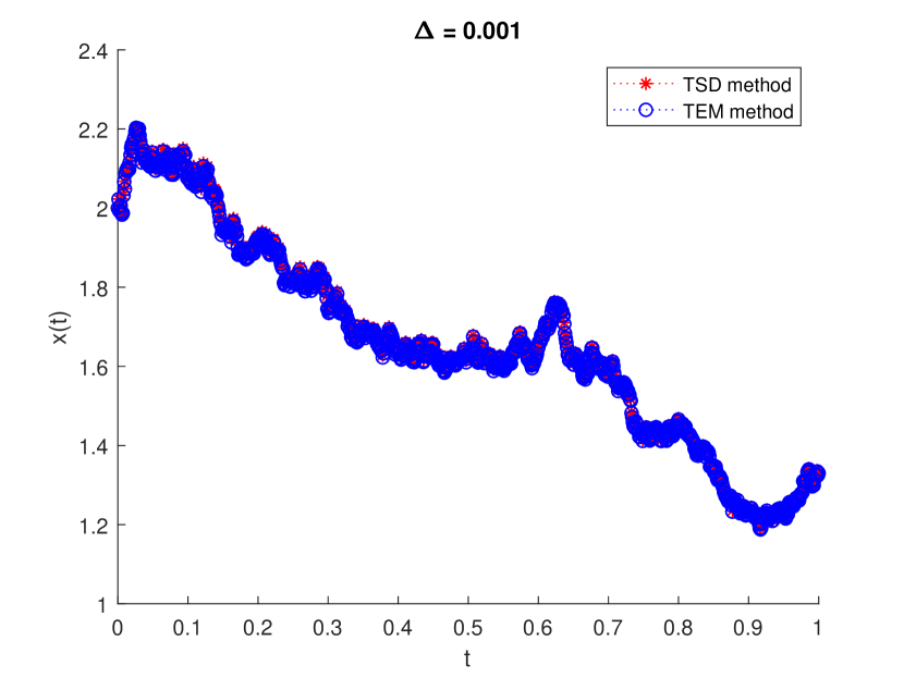
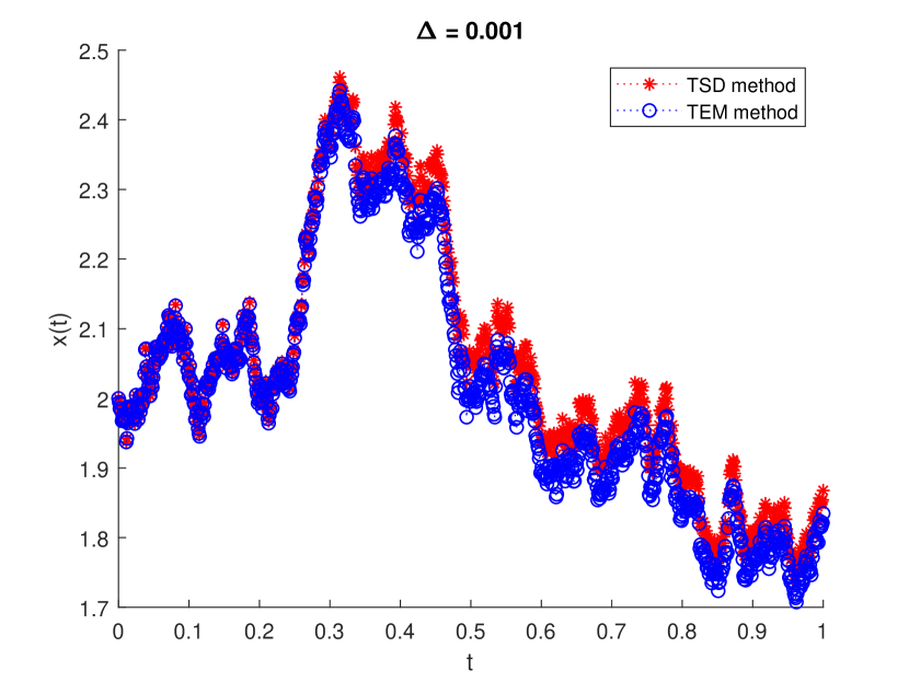
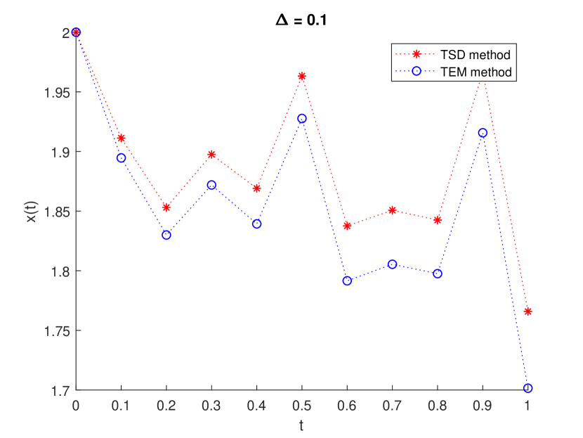
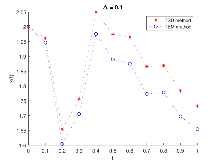
for $n\in{\mathbb{N}},$ where $\bar{h}(\Delta)=\Delta^{-\epsilon_{2}/2}$ with $\epsilon_{2}=1/2,$ and $\bar{\Delta}^{*}\leq(8\overline{C})^{-\frac{2}{\epsilon_{2}}}.$ Figure 1 shows sample simulations paths of $x(t)$ by TSD and TEM respectively with sample size $\Delta=10^{-3}.$ Note that TSD works for all $\Delta<1$ and TEM works for $\Delta\leq 0.1526$ as proved in [19]. (in an updated version of TEM in [24] it is shown that it works for all $\Delta<1$)

(a) Trajectory for (25) and (26).

(b) Trajectory for (25) and (26).

Figure 1. Trajectories of (25)-(26) for different paths of the Wiener process with $\Delta=0.001$.

(a) Trajectory for (25) and (26).

(b) Trajectory for (25) and (26).

Figure 2. Trajectories of (25)-(26) for different paths of the Wiener process with $\Delta=0.1$.

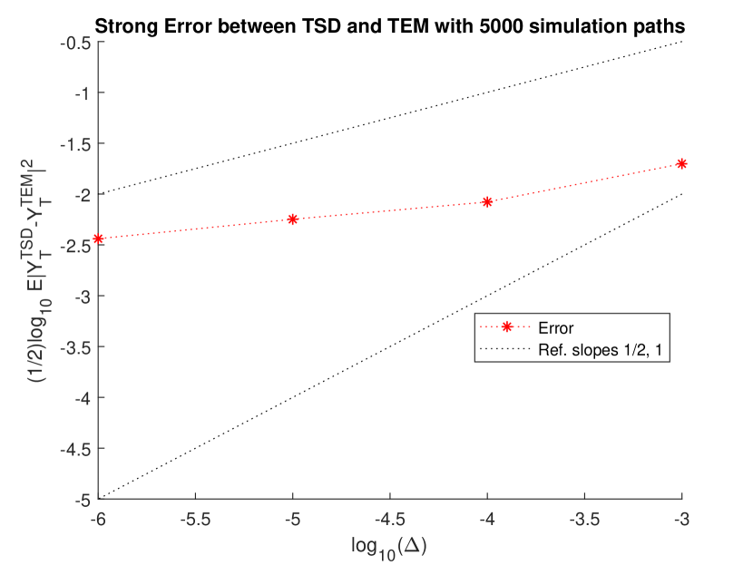
We also perform $10000$ sample paths of the TSD and TEM respectively for stepsizes $10^{-3},10^{-4},10^{-5}$ and $10^{-6}.$ Figure 3 shows the log-log plot of the strong errors between TSD and TEM which is close to $1$ TSD has order $1/2$ in ${\mathcal{L}}^{2}$-sense thus our TSD has the order $1/2$ in ${\mathcal{L}}^{2}$-sense too. Nevertheless, the approximation process TEM (26) does not always produce positive values, while TSD (25) is positive by construction.

Figure 3. The strong errors between TSD and TEM.

5. Conclusion and Future Work

In this paper we study the convergence rates of the semi-discrete (SD) method, originally proposed in [2]. Using a truncated version of the SD method, we show that the order of ${\mathcal{L}}^{2}$-convergence can be arbitrarily close to $1/2.$ The advantage of our method, over other useful numerical methods (such as the tamed Euler method, the implicit Euler method, the truncated Euler method) applied to nonlinear problems, is that it can reproduce qualitative properties of the solution process. The main qualitative property that has been investigated in all the works so far concerning the SD method is the domain preservation of the solution process. In a future work, we aim to study other qualitative properties relevant with the stability of the method and answer questions of the following type: Is the SD method able to preserve the asymptotic stability of the underlying SDE?

References

- [1] P.E. Kloeden and E. Platen. Numerical Solution of Stochastic Differential Equations, volume 23. Springer-Verlag, Berlin, corrected 2nd printing, 1995.
- [2] N. Halidias. Semi-discrete approximations for stochastic differential equations and applications. International Journal of Computer Mathematics, 89(6):780–794, 2012.
- [3] N. Halidias and I.S. Stamatiou. On the Numerical Solution of Some Non-Linear Stochastic Differential Equations Using the Semi-Discrete Method. Computational Methods in Applied Mathematics, 16(1):105–132, 2016.
- [4] N. Halidias. A novel approach to construct numerical methods for stochastic differential equations. Numerical Algorithms, 66(1):79–87, 2014.
- [5] N. Halidias. Construction of positivity preserving numerical schemes for some multidimensional stochastic differential equations. Discrete and Continuous Dynamical Systems - Series B, 20(1):153–160, 2015.
- [6] N. Halidias. Constructing positivity preserving numerical schemes for the two-factor CIR model. Monte Carlo Methods and Applications, 21(4):313–323, 2015.
- [7] N. Halidias and I.S. Stamatiou. Approximating Explicitly the Mean-Reverting CEV Process. Journal of Probability and Statistics, Article ID 513137, 20 pages, 2015.
- [8] I.S. Stamatiou. A boundary preserving numerical scheme for the Wright–Fisher model. Journal of Computational and Applied Mathematics, 328:132 – 150, 2018.
- [9] I.S. Stamatiou. An explicit positivity preserving numerical scheme for cir/cev type delay models with jump. Journal of Computational and Applied Mathematics, 360:78 – 98, 2019.
- [10] M. Hutzenthaler, A. Jentzen, and P.E. Kloeden. Strong and weak divergence in finite time of Euler’s method for stochastic differential equations with non-globally Lipschitz continuous coefficients. In Proceedings of the Royal Society of London A: Mathematical, Physical and Engineering Sciences, volume 467, pages 1563–1576. The Royal Society, 2011.
- [11] M. Hutzenthaler and A. Jentzen. Numerical approximations of stochastic differential equations with non-globally Lipschitz continuous coefficients. to appear in Memoirs of the American Mathematical Society, 236(1112), 2015.
- [12] M.V. Tretyakov and Z. Zhang. A fundamental mean-square convergence theorem for SDEs with locally Lipschitz coefficients and its applications. SIAM Journal on Numerical Analysis, 51(6):3135–3162, 2013.
- [13] Sabanis S. Euler approximations with varying coefficients: the case of superlinearly growing diffusion coefficients. Annals of Applied Probability, 26(4):2083–2105, 9 2016. 19 pages.
- [14] A. Neuenkirch and L. Szpruch. First order strong approximations of scalar SDEs defined in a domain. Numerische Mathematik, 128(1):103–136, 2014.
- [15] W. Fang and M. B. Giles. Adaptive euler–maruyama method for sdes with non-globally lipschitz drift. In Art B. Owen and Peter W. Glynn, editors, Monte Carlo and Quasi-Monte Carlo Methods, pages 217–234, Cham, 2018. Springer International Publishing.
- [16] C. Kelly and G. Lord. Adaptive time-stepping strategies for nonlinear stochastic systems. IMA Journal of Numerical Analysis, page drx036, 2017.
- [17] C. Kelly, A. Rodkina, and E. M. Rapoo. Adaptive timestepping for pathwise stability and positivity of strongly discretised nonlinear stochastic differential equations. Journal of Computational and Applied Mathematics, 334:39 – 57, 2018.
- [18] X. Mao. The truncated euler–maruyama method for stochastic differential equations. Journal of Computational and Applied Mathematics, 290:370 – 384, 2015.
- [19] X. Mao. Convergence rates of the truncated euler–maruyama method for stochastic differential equations. Journal of Computational and Applied Mathematics, 296:362 – 375, 2016.
- [20] S. Ermakov and A. Pogosian. On solving stochastic differential equations. Monte Carlo Methods and Applications, 25(2):155–161, 2019.
- [21] W. Wagner. Monte carlo evaluation of functionals of solutions of stochastic differential equations. variance reduction and numerical examples. Stochastic Analysis and Applications, 6(4):447–468, 1988.
- [22] X. Mao. Stochastic differential equations and applications. Horwood Publishing, Chichester, 2nd edition, 2007.
- [23] I. Karatzas and S.E. Shreve. Brownian motion and stochastic calculus. Springer-Verlag, New York, 1988.
- [24] L. Hu, X. Li, and X. Mao. Convergence rate and stability of the truncated euler–maruyama method for stochastic differential equations. Journal of Computational and Applied Mathematics, 337:274 – 289, 2018.