Pruning Neural Belief Propagation Decoders

Abstract

We consider near ML decoding of short linear block codes based on neural belief propagation (BP) decoding recently introduced by Nachmani et al.. While this method significantly outperforms conventional BP decoding, the underlying parity-check matrix may still limit the overall performance. In this paper, we introduce a method to tailor an overcomplete parity-check matrix to (neural) BP decoding using machine learning. We consider the weights in the Tanner graph as an indication of the importance of the connected CN to decoding and use them to prune unimportant CN. As the pruning is not tied over iterations, the final decoder uses a different parity-check matrix in each iteration. For RM and short LDPC codes, we achieve performance within $0.27\text{\,}\mathrm{dB}$ and $1.5\text{\,}\mathrm{dB}$ of the ML performance while reducing the complexity of the decoder.

I Introduction

For short code lengths, algebraic codes such as BCH codes and RM codes show excellent performance under ML decoding. However, achieving near-ML performance is computationally complex. A popular low-complexity decoding algorithm for block codes is BP decoding. For LDPC codes with sufficiently sparse parity-check matrices, BP decoding provides near-optimal performance. However, for linear block codes with dense parity-check matrices such as BCH and RM codes, the performance is not competitive. One reason for this is that the performance of BP decoding can be significantly limited by many short cycles in the graph.

Fueled by the advances in the field of deep learning, deep neural networks have also gained interest in the coding community [1, 2, 3, 4]. In [1, 2], BP decoding is formulated as a deep neural network. Instead of iterating between CN and VN, the messages are passed through unrolled iterations in a feed-forward fashion. In each iteration, the VN and CN are now referred to as VN layers and CN layers, respectively. Additionally, weights can be introduced at the edges which then are optimized using stochastic gradient descent (and variants thereof). This decoding method is commonly referred to as neural BP and can be seen as a version of WBP where each edge has a different weight. The idea is that the weights in the Tanner graph can account for short cycles and scale messages accordingly. In [3], the effects of coupling the weights over the iterations or over the nodes to reduce complexity was explored.

While WBP decoding improves upon conventional BP decoding, its performance is still limited by the underlying parity-check matrix. As the choice of the parity-check matrix is not unique, different choices of parity-check matrices may yield different performance. This fact has been exploited by using redundant parity-check matrices [5, 6, 7, 8, 9]. Kothiyal et al. combined reliability-based decoding (e.g., ordered-statistics decoding) and BP decoding in a scheme where the parity-check matrix is adapted to the outcome of the reliability-based decoding at the expense of high complexity[5]. In [6], Reed-Solomon codes are decoded iteratively by adapting the parity-check matrix in each iteration while ensuring a practical complexity. In [7], a single Tanner graph is constructed from multiple parity-check matrices based on the permutation group of the code. In [8], MBBP decoding is introduced where BP decoding is performed on multiple parity-check matrices in parallel. For RM codes, a decoder adapting the parity-check matrix depending on the location of the most reliable bits was introduced in [9].

In this paper, we introduce a pruning-based approach to selecting the best parity-check equations for each iteration of the BP decoder for short linear block codes. Our pruning-based approach starts with a large overcomplete parity-check matrix under WBP decoding. Considering the weights in the Tanner graph, the magnitude of the weights gives an indication of the importance of the edge in the decoding process. A magnitude close to zero indicate that the edge has low importance. By tying the weights for each CN, i.e., enforcing that the weights of all incoming edges to a single CN are equal, the weights can be interpreted as an indication of the importance of the CN in the decoding process. CN with connected low-weight edges do not play an important role in the decoding process and can be removed. We use this magnitude-based pruning approach to reduce the complexity of the decoder by removing CN from the Tanner graph. By allowing pruning of different CN in each iteration, the optimization results in a different parity-check equation for each iteration. The optimized parity-check matrices can be used to design decoders of different complexity, depending on the level of pruning. The weights in the corresponding Tanner graph can be untied, leading to the largest complexity. The weights obtained during the optimization process can be directly used. Alternatively, to achieve the lowest complexity, no weights at all may be used. For RM and short LDPC codes, we show that this optimization improves performance over conventional BP for the same complexity. In particular, the RM($3,7$) code performs within $0.27\text{\,}\mathrm{dB}$ of the ML performance. Also, a rate $0.5$-LDPC code of length $128$ performs within $1.5\text{\,}\mathrm{dB}$ of the ML performance, giving an improvement of $0.5\text{\,}\mathrm{dB}$ over conventional BP.

II Preliminaries

Consider a linear block code $\mathcal{C}$ of length $n$ and dimension $k$ with parity-check matrix $\bm{H}$ of size $m\times n$ where $m\geq n-k$. If $m>n-k$, we refer to the parity-check matrix as overcomplete and denote it as $\bm{H}_{\mathsf{oc}}$. We denote the corresponding Tanner graph as $\mathcal{G}=(\mathcal{V}_{\mathsf{v}},\mathcal{V}_{\mathsf{c}},\mathcal{E})$, consisting of a set of CN $\mathcal{V}_{\mathsf{c}}$, $|\mathcal{V}_{\mathsf{c}}|=m$, a set of VN $\mathcal{V}_{\mathsf{v}}$, $|\mathcal{V}_{\mathsf{v}}|=n$, and a set of edges $\mathcal{E}$ connecting CN with VN.

For each VN $v\in\mathcal{V}_{\mathsf{v}}$ we define its neighborhood

$$\mathcal{N}(v) \triangleq\mathopen{}\mathclose{{}\left\{c\in\mathcal{V}_{\mathsf{c}}:(v,c)\in\mathcal{E}}\right\},$$ (1)

i.e., the set of all CN connected to VN $v$. Equivalently, we define the neighborhood of a CN $c\in\mathcal{V}_{\mathsf{c}}$ as

$$\mathcal{N}(c) \triangleq\mathopen{}\mathclose{{}\left\{v\in\mathcal{V}_{\mathsf{v}}:(v,c)\in\mathcal{E}}\right\}.$$ (2)

Let $\lambda_{v\rightarrow c}^{(\ell)}$ and $\lambda_{c\rightarrow v}^{(\ell)}$ be the message passed from VN $v$ to CN $c$ and the message passed from CN $c$ to VN $v$, respectively, in the $\ell$-th iteration. The VN and CN updates are

$$\lambda_{v\rightarrow c}^{(\ell)} =\lambda_{\mathsf{ch},v}+\sum_{\tilde{c}\in\mathcal{N}(v)\backslash c}\lambda_{\tilde{c}\rightarrow v}^{(\ell)}$$ (3)

and

$$\lambda_{c\rightarrow v}^{(\ell)} =2\tanh^{-1}\mathopen{}\mathclose{{}\left(\prod_{\tilde{v}\in\mathcal{N}(c)\backslash v}\tanh\mathopen{}\mathclose{{}\left(\frac{1}{2}\lambda_{\tilde{v}\rightarrow c}^{(\ell)}}\right)}\right),$$ (4)

respectively, where $\lambda_{\mathsf{ch},v}$ is the LLR of the channel output. For bipolar transmission over the additive white Gaussian noise channel, it follows that

$$\lambda_{\mathsf{ch},v} \triangleq\ln\frac{p_{Y|B}(y_{v}|b_{v}=0)}{p_{Y|B}(y_{v}|b_{v}=1)}\overset{}{=}\frac{2y_{v}}{\sigma^{2}}$$ (5)

where $y_{v}$ is the channel output, $b_{v}$ is the transmitted bit, and $\sigma^{2}$ is the variance of the noise. The VN output LLR in the $\ell$-th iteration is

$$\lambda_{v}^{(\ell)} =\lambda_{\mathsf{ch},v}+\sum_{\tilde{c}\in\mathcal{N}(v)}\lambda_{\tilde{c}\rightarrow v}^{(\ell)}.$$ (6)

II-A Weighted Belief Propagation

One way to counteract the effect of short cycles on the BP decoding performance is to introduce weights for each edge in the Tanner graph [1, 2] which is referred to as neural BP and can be seen as version of WBP where each edge has an individual weight. For WBP, the update rules ([eq:vn_update]3) and ([eq:cn_update]4) modify to

$$\lambda_{v\rightarrow c}^{(\ell)} =w_{v}^{(\ell)}\lambda_{\mathsf{ch},v}+w_{v\rightarrow c}^{(\ell)}\sum_{\tilde{c}\in\mathcal{N}(v)\backslash c}\lambda_{\tilde{c}\rightarrow v}^{(\ell)}.$$ (7)

and

$$\lambda_{c\rightarrow v}^{(\ell)} =2w_{c\rightarrow v}^{(\ell)}\tanh^{-1}\mathopen{}\mathclose{{}\left(\prod_{\tilde{v}\in\mathcal{N}(c)\backslash v}\tanh\mathopen{}\mathclose{{}\left(\frac{1}{2}\lambda_{\tilde{v}\rightarrow c}^{(\ell)}}\right)}\right)$$ (8)

where $w_{v}^{(\ell)}$, $w_{v\rightarrow c}^{(\ell)}$, and $w_{c\rightarrow v}^{(\ell)}$, are the channel, VN, and CN weights, respectively. The VN output LLR in the $\ell$-th iteration is

$$\lambda_{v}^{(\ell)} =w_{v}^{(\ell)}\lambda_{\mathsf{ch},v}+w_{v\rightarrow c}^{(\ell)}\sum_{\tilde{c}\in\mathcal{N}(v)}\lambda_{\tilde{c}\rightarrow v}^{(\ell)}.$$ (9)

Update rules ([eq:vn_update_wbp]7) and ([eq:cn_update_wbp]8) describe WBP when the weights are untied over all nodes as well as over all iterations. In order to reduce complexity, the weights can also be tied. In [3], tying weights temporally, i.e., over iterations, and tying the weights spatially, i.e., within one node layer, was explored.

Here, we consider the case where the weights in each CN are tied, i.e., $w_{c}^{(\ell)}=w_{c\rightarrow v}^{(\ell)}$ for all $v\in\mathcal{N}(c)$. Hence, the CN update results to

$$\lambda_{c\rightarrow v}^{(\ell)} =2w_{c}^{(\ell)}\tanh^{-1}\mathopen{}\mathclose{{}\left(\prod_{\tilde{v}\in\mathcal{N}(c)\backslash v}\tanh\mathopen{}\mathclose{{}\left(\frac{1}{2}\lambda_{\tilde{v}\rightarrow c}^{(\ell)}}\right)}\right).$$ (10)

Note that setting all the weights of a WBP decoder to one results in conventional BP decoding.

II-B Optimization of the Weights

The decoding process can be seen as a classification task where the channel output is mapped to a valid codeword. This task consists of $2^{k}$ classes, one for each codeword. Training such a classification task is unfeasible as the resulting decoder generally generalizes poorly to classes not contained in the training data [4]. Instead, the task can be reduced to binary classification for each of the $n$ bits. As a loss function, the bitwise cross-entropy between the transmitted codeword and the VN output LLR of the final VN layer was used in [1, 2]. The optimization behavior can be improved by using a multiloss, where the overall loss is the average bitwise cross-entropy between the transmitted codeword and the VN output LLR of each VN layer.

In [3], it was observed that the binary-cross entropy does not perform well for large, overcomplete parity-check matrices. Wrongly decoded bits with large LLR result in large cross-entropy losses and cause the training to converge slowly. As an alternative, the loss function

$$\Gamma =\frac{1}{n}\sum_{v=1}^{n}(1-o_{v})^{x_{v}}o_{v}^{1-x_{v}}$$ (11)

was proposed, where $o_{v}^{(\ell)}$ is the estimate of the probability that the $v$-th bit in the $\ell$-th iteration is one, i.e., $o_{v}^{(\ell)}=\sigma(\lambda_{v}^{(\ell)})=1/(1+\mathrm{exp}(-\lambda_{v}^{(\ell)}))$. Since substituting hard-decision values for $o_{v}^{(\ell)}$ results in the bit-error rate, ([eq:soft_ber]11) is referred to as soft bit-error rate. Combining the soft bit-error rate and a multiloss results to

$$\tilde{\Gamma} =\frac{1}{\sum\eta^{L-\ell}}\sum_{t=1}^{L}\eta^{L-\ell}\frac{1}{n}\sum_{v=1}^{n}\mathopen{}\mathclose{{}\left(1-o_{v}^{(\ell)}}\right)^{x_{v}}\mathopen{}\mathclose{{}\left(o_{v}^{(\ell)}}\right)^{1-x_{v}}$$ (12)

$$\overset{(a)}{=}\frac{1}{\sum\eta^{L-\ell}}\sum_{\ell=1}^{L}\eta^{L-\ell}\frac{1}{n}\sum_{v=1}^{n}o_{v}^{(\ell)}$$ (13)

where $\eta$ determines the contribution of intermediate layers to the overall loss and is decreased during the training, such that in the final phase of the training only the last layer contributes to the loss [3]. Step $(a)$ follows from the fact that since the channel and the decoder are symmetric, the all-zero codeword can be used for training.

III Optimizing the Parity-Check Matrix

While WBP decoding as described in the previous section improves upon conventional BP decoding, its performance is quite dependent on the choice of the parity-check matrix. Here, we propose a pruning-based approach to select the relevant parity-checks from a large, overcomplete parity-check matrix. For this, we consider a modified WBP where the weights are tied at the CN, i.e., all messages at a single CN are weighted by the same weight $w_{c}^{(\ell)}$ as in ([eq:cn_update_pp]10). The VN update ([eq:vn_update_wbp]7) remains unchanged. The magnitude of the weights $w_{c}^{(\ell)}$ can now be interpreted as a measure of how much the CN contributes to decoding. A large magnitude indicates high importance whereas a magnitude of zero indicates that the CN is irrelevant to the decoding process.

III-A Training Procedure

Let $\mathcal{H}=\{\bm{H}_{1},\ldots,\bm{H}_{L}\}$ be a set of parity-check matrices where $\bm{H}_{\ell}$ is the parity-check matrix used for decoding in the $\ell$-th iteration. Equivalently, we define a set of weights $\mathcal{W}$. The set of parity-check matrices is initialized with the same large overcomplete matrix $\bm{H}_{\mathsf{oc}}$ for each iteration, i.e., $\bm{H}_{\ell}=\bm{H}_{\mathsf{oc}}$, $\ell=1,\ldots,L$. All weights are initialized to one, i.e., we start with conventional BP. The weights in $\mathcal{W}$ are then optimized using the Adam optimizer [10] within the Tensorflow programming framework [11]. After the optimization has converged, we find the index and the iteration of the lowest CN weight $w_{c}^{(\ell)}$ and set it to zero, i.e., we prune the corresponding parity-check equation from $\mathcal{W}$. As this may change the optimal value for the remaining weights, we rerun the training. We iterate between retraining and pruning CN until we either reach a desired number of parity-check equations or until the loss starts diverging. The result of the optimization is a set of parity-check equations $\mathcal{H}_{\mathsf{opt}}=\mathopen{}\mathclose{{}\left\{\bm{H}_{\ell,\mathsf{opt}}}\right\}$ with $\ell=1,\ldots,L$ and optimized weights $\mathcal{W}_{\mathsf{opt}}$. The training process is illustrated in the flowchart of Fig. [fig:training]1.

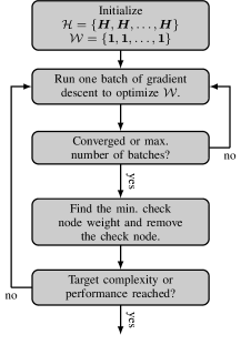
Figure 1: Flowchart of the training process.

III-B Complexity Discussion

In the BP decoder, the evaluation of the $\tanh$ and inverse $\tanh$ functions is the operation of highest computational complexity. It is natural to use the number of these evaluations as a measure of the complexity of the decoder. As both functions are evaluated in the CN, it is equivalent to use the number of CN and hence the number of parity-check equations, i.e., rows in the parity-check matrix. The required memory is related to the parity-check matrix itself and the number of weights. Since the weights are real numbers as opposed to binary values for the edges, we quantify memory requirements with the number of weights.

With this, we define three decoders of different complexity.

• Decoder $\mathcal{D}_{1}$: It uses the result from the optimization directly, i.e., $\mathcal{H}_{\mathsf{opt}}$ and $\mathcal{W}_{\mathsf{opt}}$. Hence, it uses ([eq:vn_update_wbp]7) and ([eq:cn_update_pp]10) as updates in the respective nodes.

• Decoder $\mathcal{D}_{2}$: It uses the optimized set of parity-check matrices, i.e., $\mathcal{H}_{\mathsf{opt}}$, but sets all weights to one, i.e., neglects $\mathcal{W}_{\mathsf{opt}}$. It uses ([eq:vn_update]3) and ([eq:cn_update]4) as updates in the respective nodes.

• Decoder $\mathcal{D}_{3}$: It uses the optimized set of parity-check matrices, i.e., $\mathcal{H}_{\mathsf{opt}}$, and additionally untied optimized weights over all iterations and edges as in [1]. Hence, the updates rules become ([eq:vn_update_wbp]7) and ([eq:cn_update_wbp]8) in the respective nodes. It is important to note that to obtain the untied weights, an extra training step with untied weights is required as previously we only considered tied weights in the CN.

Concerning the decoders, all three have similar computational complexity as they operate on the same set of parity-check matrices. However, they differ in the required memory. Decoder $\mathcal{D}_{3}$ needs to store the most weights, i.e., one weight per edge, whereas $\mathcal{D}_{2}$ does not need to store any weights. Decoder $\mathcal{D}_{1}$ only needs to store one weight per CN and hence is of lower complexity than $\mathcal{D}_{3}$ but higher complexity than $\mathcal{D}_{2}$.

IV Numerical Results

We numerically evaluate the performance of the proposed parity-check matrix optimization for RM codes and a short LDPC code. As a benchmark we consider ML decoding.

IV-A The RM Code RM$(2,5)$

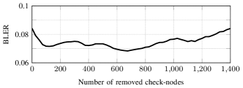
Figure 2: BLER at $3\text{\,}\mathrm{dB}$ during the training process for the RM$(2,5)$ code.

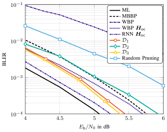
Figure 3: BLER results for the RM$(2,5)$ code.

The RM$(2,5)$ code has $620$ parity-check equations of minimum weight that are used to initialize the optimization. We fix the number of iterations to six. Hence, $620$ CN need to be evaluated per iteration which leads to a total of $3720$ CN that need to be evaluated. The optimization is stopped when the loss starts to increase. In total, $31\text{\,}\mathrm{\char 37\relax}$ of the parity-check equations remain. In Fig. [fig:pruning_rm_2_5]2, we depict the BLER as a function of removed CN. In Fig. [fig:bler_rm_2_5]3, we plot the BLER as a function of $E_{\mathsf{b}}/N_{0}$. Decoder $\mathcal{D}_{1}$ performs within $0.38\text{\,}\mathrm{dB}$ of the ML decoder at a BLER of $10^{-4}$. Removing the weights from the optimized parity-check matrix ($\mathcal{D}_{2}$), results in a penalty of $0.48\text{\,}\mathrm{dB}$. Untying the weights in the CN ($\mathcal{D}_{3}$) results in an additional gain of $0.047\text{\,}\mathrm{dB}$ with respect to $\mathcal{D}_{2}$.

Both $\mathcal{D}_{1}$ and $\mathcal{D}_{3}$, requiring $1170$ CN, outperform WBP [1] with $\bm{H}_{\mathsf{oc}}$ containing the $620$ parity-check equations of minimum weight and hence $3720$ CN, as well as MBBP [8] with $15$ randomly chosen parity-check matrices with $1440$ CN. Only $\mathcal{D}_{2}$ performs slightly worse, but at the same time requires only $1170$ CN and no weights. A recurrent neural network (RNN)-based decoder as introduced in [2] using $\bm{H}_{\mathsf{oc}}$ slightly outperforms $\mathcal{D}_{1}$ and $\mathcal{D}_{2}$ at the cost of increased complexity by about three times. WBP [1] with a standard parity-check matrix containing $16$ CN is clearly not competitive. The decoding complexity of the decoders in Fig. [fig:bler_rm_2_5]3 is reported in Table [tab:complexity]LABEL:tab:complexity.

To verify the effectiveness of our pruning strategy for CN, we also consider the scenario where we randomly prune CN. As it can be observed in Fig. [fig:bler_rm_2_5]3, this approach is clearly not competitive.

To investigate the behavior of the pruning, we are interested how many CN are pruned in each BP iteration, or equivalently, how many CN remain. To this end, we plot the fraction of all remaining CN per iteration in Fig. [fig:rm_2_5_cn_fraction]4. We observe that in the first BP iteration, about $40\text{\,}\mathrm{\char 37\relax}$ of all remaining CN are used for decoding. In later BP iterations, the number of CN decreases significantly. This observation furthermore justifies the use of a low number of iterations.

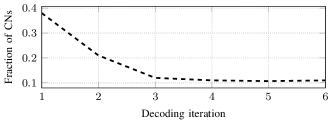
Figure 4: Fraction of the remaining CN after pruning used for decoding in the respective iteration for the RM$(2,5)$ code.

[ caption = Complexity of the decoders for different codes., label = tab:complexity, pos = tb, doinside = , ]lcr & # of CN evaluations WBP, RM$(2,5)$ $16\cdot 6=96$WBP, RNN $\bm{H}_{\mathsf{oc}}$, RM$(2,5)$ $620\cdot 6=3720$MBBP RM$(2,5)$ $15\cdot 6\cdot 16=1440$ $\mathcal{D}_{1}$, $\mathcal{D}_{2}$, $\mathcal{D}_{3}$, RM$(2,5)$ $620\cdot 6\cdot 0.31=1170$Random, RM$(2,5)$ $620\cdot 6\cdot 0.31=1170$WBP, RNN $\bm{H}_{\mathsf{oc}}$, RM$(3,7)$ $94488\cdot 6=566928$MBBP RM$(3,7)$ $60\cdot 6\cdot 64=23440$ $\mathcal{D}_{1}$, $\mathcal{D}_{2}$, $\mathcal{D}_{3}$, RM$(3,7)$ $94488\cdot 6\cdot 0.03=19842$$\mathcal{\tilde{D}}_{1}$, RM$(3,7)$ $9448\cdot 6\cdot 0.35=19842$BP, CCSDS, 25 iterations $64\cdot 25=1600$BP, CCSDS, 100 iterations $64\cdot 100=6400$WBP, CCSDS $64\cdot 6=96$$\mathcal{D}_{1}$, $\mathcal{D}_{3}$ CCSDS $10000\cdot 6\cdot 0.027=1600$

IV-B The RM Code RM$(3,7)$

The RM$(3,7)$ code has $94488$ parity-check equations of minimum weight. In the initial training phases, optimizing the weights converges very slowly and removing CN is done in an almost random fashion. To speed up the training for decoders $\mathcal{D}_{1}$, $\mathcal{D}_{2}$, and $\mathcal{D}_{3}$, we randomly select $70000$ parity-check equations and use them as the overcomplete parity-check matrix $\bm{H}_{\mathsf{oc}}$. Decoder $\mathcal{\tilde{D}}_{1}$ uses only a small, random subset, namely $9448$, of all parity-check equations of minimum weight as the overcomplete parity-check matrix $\bm{H}_{\mathsf{oc}}$. For all four decoders, we consider six iterations.

In Fig. [fig:bler_rm_3_7]5, we plot the BLER. Decoder $\mathcal{D}_{1}$ performs within $0.27\text{\,}\mathrm{dB}$ of the ML decoder. Removing the weights results in a degradation of $0.47\text{\,}\mathrm{dB}$ for decoder $\mathcal{D}_{2}$ with respect to $\mathcal{D}_{1}$. On the other hand, untying the weights results in a gain of $0.02\text{\,}\mathrm{dB}$ for decoder $\mathcal{D}_{3}$. Decoders $\mathcal{D}_{1}$, $\mathcal{D}_{2}$, and $\mathcal{D}_{3}$, all require $19842$ CN and outperform MBBP with $60$ randomly chosen parity-check matrices, i.e., $23440$ CN, and WBP as in [1] with $\bm{H}_{\mathsf{oc}}$ and the RNN-based decoder [2] with $\bm{H}_{\mathsf{oc}}$ while having lower complexity. As for the RM$(2,5)$ code, WBP over the standard parity-check matrix with $64$ CN is not competitive (curve omitted for better readability). The complexities are reported in Table [tab:complexity]LABEL:tab:complexity.

Decoder $\mathcal{\tilde{D}}_{1}$ demonstrates the effect of using only a small subset of all parity-check equations of minimum weight as the overcomplete parity-check matrix $\bm{H}_{\mathsf{oc}}$. In this case, only $9448$ randomly chosen parity-check equations were used initially and the decoder is pruned to the same complexity as $\mathcal{D}_{1}$. This essentially corresponds to randomly pruning CN and results in the same performance degradation as for the RM$(2,5)$ code.

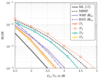
Figure 5: BLER results for the RM$(3,7)$ code.

IV-C Low-Density Parity-Check Code

We consider the CCSDS LDPC code of length $128$ and rate $0.5$ as defined in [12]. It has a CN degree of $8$ with half the VN having degree $3$ and half having degree $5$. The code has a minimum distance $14$. For decoding, $25$ iterations are used. Hence, a total of $1600$ CN updates are required.

For the overcomplete matrix, we start with $10000$ randomly chosen parity-check equations of low or minimum weight. Then, we prune the decoder to the same complexity as conventional BP decoding, i.e., we allow $1600$ CN updates. The number of iterations is set to six. Both decoders $\mathcal{D}_{1}$ and $\mathcal{D}_{3}$ outperform conventional BP by approximately $0.6\text{\,}\mathrm{dB}$. Allowing $100$ iterations for conventional BP shows that the gain of decoders $\mathcal{D}_{1}$ and $\mathcal{D}_{3}$ decreases to $0.2\text{\,}\mathrm{dB}$. However, conventional BP with $100$ iterations requires $6400$ CN and therefore has a higher complexity than decoders $\mathcal{D}_{1}$ and $\mathcal{D}_{3}$. WBP [1] with $64$ CN is again not competitive. The complexities are reported in Table [tab:complexity]LABEL:tab:complexity.

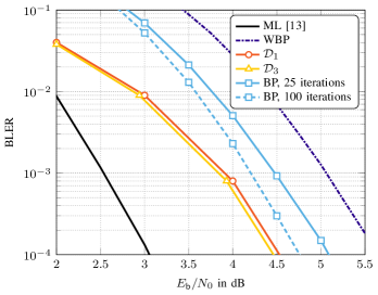
Figure 6: BLER results for the LDPC code.

V Conclusion

We applied machine learning to optimize the parity-check matrix for conventional and weighted belief propagation decoding. To this end, we prune a large overcomplete parity-check matrix and allow it to consist of different parity-check equations in each iteration. We obtain significant performance gains while keeping the complexity practical. For RM and short, standardized LDPC codes we demonstrated a performance within up to $0.27\text{\,}\mathrm{dB}$ and $1.5\text{\,}\mathrm{dB}$ of ML decoding, respectively. In all scenarios, our approach outperforms conventional BP while having equal complexity and MBBP and the original neural BP while even allowing lower complexity. Our approach can easily be applied to any other linear block code such as BCH codes and similar gains over conventional BP decoding are expected.

References

- [1] E. Nachmani, Y. Be’ery, and D. Burshtein, “Learning to decode linear codes using deep learning,” in Proc. Annu. Allerton Conf. Commun., Control, Comput., Allerton, IL, USA, Sep. 2016, pp. 341–346.
- [2] E. Nachmani, E. Marciano, L. Lugosch, W. J. Gross, D. Burshtein, and Y. Be’ery, “Deep learning methods for improved decoding of linear codes,” IEEE J. Sel. Topics Signal Process., vol. 12, no. 1, pp. 119–131, Feb. 2018.
- [3] M. Lian, F. Carpi, C. Häger, and H. D. Pfister, “Learned belief-propagation decoding with simple scaling and SNR adaptation,” in Proc. IEEE Int. Symp. Inf. Theory, Paris, France, Jul. 2019, pp. 161–165.
- [4] T. Gruber, S. Cammerer, J. Hoydis, and S. ten Brink, “On deep learning-based channel decoding,” in Proc. Annu. Conf. Inf. Sci. Syst., Baltimore, MD, USA, May 2017.
- [5] A. Kothiyal, O. Y. Takeshita, W. Jin, and M. Fossorier, “Iterative reliability-based decoding of linear block codes with adaptive belief propagation,” IEEE Commun. Lett., vol. 9, no. 12, pp. 1067–1069, Dec. 2005.
- [6] J. Jiang and K. R. Narayanan, “Iterative soft-input soft-output decoding of Reed-Solomon codes by adapting the parity-check matrix,” IEEE Trans. Inf. Theory, vol. 52, no. 8, pp. 3746–3756, Aug. 2006.
- [7] T. R. Halford and K. M. Chugg, “Random redundant soft-in soft-out decoding of linear block codes,” in Proc. IEEE Int. Symp. Inf. Theory, Seattle, WA, USA, Jun. 2006, pp. 2230–2234.
- [8] T. Hehn, J. Huber, O. Milenkovic, and S. Laendner, “Multiple-bases belief-propagation decoding of high-density cyclic codes,” IEEE Trans. Commun., vol. 58, no. 1, pp. 1–8, Jan. 2010.
- [9] E. Santi, C. Häger, and H. D. Pfister, “Decoding Reed-Muller codes using minimum- weight parity checks,” in Proc. IEEE Int. Symp. Inf. Theory, Vail, CO, USA, Jun. 2018, pp. 1296–1300.
- [10] D. P. Kingma and J. Ba, “Adam: A method for stochastic optimization,” in Proc. Int. Conf. Learning Representations, San Diego, CA, USA, May 2015, pp. 1–15.
- [11] M. Abadi et al. (2015) TensorFlow: Large-scale machine learning on heterogeneous systems. [Online]. Available: https://www.tensorflow.org/
- [12] “Short block length LDPC codes for TC synchronization and channel codding (CCSDS 231.1-O-1),” Consultative Committee for Space Data Systems (CCSDS), Tech. Rep., Apr. 2015.
- [13] M. Helmling, S. Scholl, F. Gensheimer, T. Dietz, K. Kraft, S. Ruzika, and N. Wehn, “Database of channel codes and ML simulation results,” www.uni-kl.de/channel-codes, 2019.