Balancing domain decomposition by constraints associated with subobjects
Abstract
A simple variant of the BDDC preconditioner in which constraints are imposed on a selected set of subobjects (subdomain subedges, subfaces and vertices between pairs of subedges) is presented. We are able to show that the condition number of the preconditioner is bounded by , where is a constant, and and are the characteristic sizes of the mesh and the subobjects, respectively. As can be chosen almost freely, the condition number can theoretically be as small as . We will discuss the pros and cons of the preconditioner and its application to heterogeneous problems. Numerical results on supercomputers are provided.
keywords:
BDDC , FETI-DP , optimal preconditioner , parallel solver , heterogeneous problemsMSC:
[2010] 65N55 , 65N22 , 65F081 Introduction
It is well-known in the literature [12, 13, 14, 16, 8, 7] that the condition number of the BDDC method and the closely related FETI-DP method is bounded by , where is a constant, and and are the characteristic sizes of the subdomain and the mesh, resp. Consequently, when the mesh and its partition are fixed, users can only vary the number of constraints to adjust the convergence rate.
Traditionally, these constraints are values at subdomain corners, or average values on subdomain edges or faces. In the perturbed formulation of BDDC [6, 5], any combination of vertex, edge or face constraints can be used. Normally, these combinations provide enough options for users to choose their desired convergence rate. However, for difficult problems, such as the ones with heterogeneous diffusion coefficients, see, e.g., [1], the convergence of the BDDC method [9] can be unsatisfied even if all possible constraints are used.
In this work, we propose to impose constraints on coarse objects (subdomain subedges and subfaces, and vertices between subedges) that are adapted to the local mesh size and to the user’s desired rate of convergence. We refer to this new variant as BDDC-SO. If is the characteristic size of the objects, we can prove that the conditioned number of the BDDC-SO preconditioned operator is bounded by
As can be as small as , there is no restriction in the rate of convergence of BDDC-SO. However, the trade-off is having to solve larger coarse problems. Therefore, the BDDC-SO can be seen as a standalone method for small to medium problems (tested up to 260 million unknowns on 8K processors), or as a proven, simple approach to improve the rate of convergence. In addition, BDDC-SO is perfectly robust w.r.t. the variation of the diffusion coefficient when coarse objects are chosen such that the coefficient associated with each object is constant or varies mildly. BDDC-SO also has great potentials to be extended to multi-level.
2 Model problem and abstract multispace BDDC framework
Let be a bounded domain in . We consider the Poisson’s equation with homogeneous Dirichlet conditions. Its weak formulation reads as follows: find such that
| (1) |
where
Let be a shape-regular mesh of with characteristic mesh size , and be the corresponding Finite Element (FE) space of continuous piecewise linear functions that vanish on . Then the discrete problem associated with (1) is to find such that
| (2) |
We quote the following definition of the abstract multispace BDDC preconditioner from [15].
Definition 1
Assume that is defined and symmetric semipositive definite on some larger space and there exist subspaces and projections , , such that are a-orthogonal, i.e., for , is positive definite on each , and
Then the abstract multispace BDDC preconditioner is defined by
3 Balancing domain decomposition by constraints associated with subobjects
We will present the formulation of our proposed BDDC preconditioner using the abstract BDDC framework introduced in Section 2. First, we consider a partition of into non-overlapping open subdomains. We further assume that every subdomain is a union of elements in and is connected. Let be the interface of . For each , let be the space of FE functions which vanish on . We define and note that functions in can be discontinuous across .
Let be the extension of on associated with : . Denote by the space of functions in that are zero on . Let be the -orthogonal projection from onto . The functions in are called discrete harmonic. They are -orthogonal with functions in and they possess the smallest energy among functions in having the same values on .
Given a mesh partition, the BDDC method is characterized by the selection of certain coarse degrees of freedom and some weighting operator that projects functions in onto .
Coarse degrees of freedom are usually defined as functionals, which are values at or averages over some geometrical coarse objects. In the standard BDDC method, these coarse objects are vertices and/or edges and/or faces of subdomains. For systematic ways of classifying degrees of freedom into objects, we refer the reader to [10, 1].
In this work, we propose to further partition edges and faces of the subdomains into subedges, subfaces and vertices between pairs of subedges. One way to obtain this is to partition each subdomain into smaller subsubdomains. These new subsubdomains together form a new partition of . Denote by the interface of , we emphasize that . The BDDC-SO method selects objects from the set of subdomain vertices, edges and faces of to define its coarse degrees of freedom. A simple example in 2D is illustrated in Figure 1. On the left, standard coarse objects consisting of a vertex and four edges are shown. On the right, obtained from a finer partition , we have 8 subedges and 5 vertices between them. We emphasize that one normally does not have to impose constraints on all available objects.
Remark 2
The decision to break each original subdomain into smaller subsubdomains can be made locally in practice. However, in order to classify degrees of freedom (DOFs) into subobjects, see, e.g., [11, 1], one needs to know the list of subsubdomains each interface DOF belongs to. In a distributed-memory context, this can be obtained after a cheap nearest-neighbor communication sweep among original subdomains.
Let be the BDDC space (of BDDC-SO) consisting of functions in that have common values (continuous) at the selected coarse degrees of freedom. As we use a finer partition of the interface, the BDDC space associated with BDDC-SO is generally a subspace of the one associated with the standard BDDC.
Next, let be the weighting operator (projection) from onto , that takes weighted average of contributions from subdomains, more precisely
| (3) |
Here denotes the cardinality of the set . In general, the weight defined by (3) is the same as the usual multiplicity weighting in, e.g., [16]. However, for some (but not all) DOFs on the interface of the partition , the two weightings can be different. An example of such a DOF is depicted in Figure 1 with a big solid dot and labeled as . For this particular DOF,
while its multiplicity weight would be .
4 Convergence Analysis
In order to establish the condition number bound for the BDDC-SO preconditioner, we consider an auxiliary BDDC preconditioner, BDDC-A. This preconditioner is constructed similar to BDDC-SO using the abstract multispace framework introduced in Section 2. However, there are three fundamental differences. First, BDDC-A is defined on the partition introduced in Section 3 to form subobjects. This partition has characteristic size . The new partition leads to a larger space of discontinuous functions and a different projection onto the space of inner functions associated with . Second, coarse objects of BDDC-A are chosen such that it shares the same BDDC space with BDDC-SO. This is done as follows: i) on , subobjects of BDDC-SO, which are associated with regular geometrical objects (vertices, edges and faces of subsubdomains ), are selected, ii) on , each degree of freedom is treated as a vertex. In other words, we impose full continuity on the part of the interface outside of . Third, the weighting operator is the standard counting weighting operator defined by
| (4) |
Let be the extension of on associated with . The following is our main result.
Theorem 3
The condition number of the BDDC-SO preconditioner is bounded by
| (5) |
Proof 1
Since the formulation of BDDC-SO follows the abstract framework of multispace BDDC, its condition number can be bounded as in the first inequality in (5), see [13, 15]. In addition, as BDDC-A is a standard BDDC preconditioner with regular coarse objects, standard weighting operator, and defined on the partition having characteristic size , the third inequality in (5) is a standard result (see [13, 15]). We only need to prove the second inequality in (5).
First, we note that can be discontinuous across but is always continuous in each . Therefore, for all . Second, as and are projections onto the space of inner functions that respectively vanish on and , we have . On the other hand, is discrete harmonic in with partition . This implies that it has the smallest -norm among functions in which share its value on . In other words,
Here, we note that the last equality is due to the fact that is continuous in each . This finishes the proof.
Remark 4
The BDDC-SO preconditioner can be extended to the case with variable diffusion coefficients, i.e., when the bilinear form becomes , where varies from element to element. As our analysis relies on the convergence of the auxiliary preconditioner BDDC-A, the subobjects need to be chosen in such a way that the coefficient has to be constant in each subsubdomain . In addition, the weighting operator in (3) needs to be updated to incorporate with We have explored this direction and obtained first results for multi-material problems in [1].
Remark 5
As the proof of Theorem 3 is based on the standard result for an auxiliary BDDC preconditioner, we need to fulfill all requirements of that result [12, 16]. Among these requirements, it is crucial to have enough primal constraints (the constraints we actually impose on subobjects) so that for every pair of neighboring subsubdomains, there exists an acceptable path, see [12, 16, 11, 1]. In general, we can guarantee the existence of acceptable paths by choosing either all edge or all face subobjects on the original interface. Using all the possible vertex constraints also leads to a scalable preconditioner but is less common in practice due to its poor performance, especially in 3D, see, e.g.,[16]. For algorithms to find close-to-minimal set of primal constraints, we refer the reader to [11, 1].
5 Numerical Experiments
The standard BDDC and BDDC-SO preconditioners have been implemented in FEMPAR, a parallel framework for the massively parallel FE simulation of multiphysics problems governed by PDEs [4, 3]. We will test these preconditioners on MareNostrum 4 at Barcelona Supercomputing Center on the Poisson problem (1) with , the unit cube, and Dirichlet boundary conditions imposed on the whole boundary of .
5.1 A preconditioner with condition number
| number of iterations | size of the coarse problem | |||||||||||
| Local problem size () | 4 | 8 | 16 | 24 | 32 | 4 | 8 | 16 | 24 | 32 | ||
| BDDC(vef) | 5 | 6 | 9 | 10 | 11 | 5,859 | 5,859 | 5,859 | 5,859 | 5,859 | ||
| BDDC-SO(vef) | 4 | 4 | 4 | 4 | 4 | 5,859 | 32,319 | 150,039 | 354,159 | 532,269 | ||
| BDDC-SO(vf-min) | 5 | 4 | 4 | 4 | 4 | 2,304 | 13,259 | 53,919 | 146,979 | 236,439 | ||
In the first experiment, which is a proof of concept of the result in Theorem 3, we solve the problem on a set of uniform meshes with hexahedra, where . We use processors, each of which is responsible for a local problem of size cells. In Table 1, we report the number of PCG iterations required to reduce the 2-norm of the residual by a factor of using BDDC and BDDC-SO preconditioners. For both of them, vertex, edge and face constraints (vef) will be used. For BDDC-SO, as the meshes get finer and finer we will use smaller subobjects to keep the ratio constant (). We can see that, even when all the possible constraints are used, the number of iterations of BDDC(vef) method increases as the local problem size increases. The number of iterations of BDDC-SO(vef), on the other hand, remains constant throughout. In addition, even when we drop edge constraints and only use half of the face constraints (vf-min), the number of iterations is still the same except for . These results confirm the estimate in (5) and indicate that one does not need to impose constraints on all available subobjects to achieve the desired rate of convergence.
5.2 3D channels problem
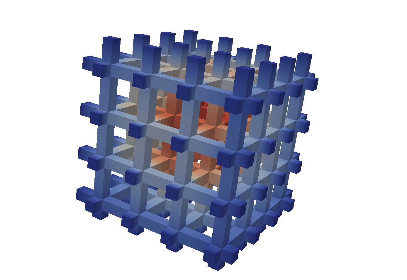
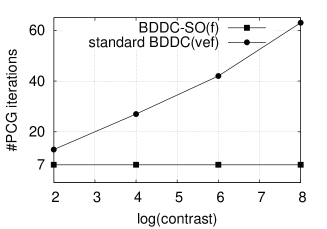
In practice, we rarely want to keep small at all cost as in Section 5.1 because the size of the coarse problem could be prohibitively large. In many situations, an introduction of a relatively small number of subobjects can greatly improve the convergence. In order to demonstrate that, we consider (1) with the modification described in Remark 4. We assume that the material has the background with and a system of channels with high diffusion coefficient , see Figure 2 (left). First, we test the robustness of the two preconditioners when solving a small problem with the mesh of hexahedra partitioned into subdomains. For BDDC-SO, each subdomain is split into two smaller subdomains, one associated with the background and the other associated with the channels. These smaller subdomains form the fine partition to define the subobjects. In Figure 2 (right), we plot the number of PCG iterations required by standard BDDC using all possible vertex, edge and face constraints (BDDC(vef)), and BDDC-SO using only face constraints (BDDC-SO(f)) to reduce the 2-norm of the residual by a factor of . We can see that while the number of iterations of BDDC(vef) increases significantly as the contrast () increases, the number of iterations of BDDC-SO(f) is constant throughout. This verifies that BDDC-SO can be very robust for heterogeneous material problems.
Next, we consider . We build uniform meshes with hexahedra. The largest mesh has more than 260 million grid points. These meshes are partitioned into regular partitions of subdomains, for . The subobjects of BDDC-SO are defined similarly. In Figure 3, we present the weak scalability study in both PCG number of iterations and time (in seconds) of standard BDDC and BDDC-SO. For each preconditioner, we consider two variants: one using vertex and edge constraints (ve), the other using vertex, edge and face constraints (vef). We can observe excellent weak scalability and robustness of BDDC-SO (bottom row). On the other hand, the performance of standard BDDC (top row) varies widely as the number of processors increases. BDDC-SO methods are also much faster. They require less than 21 iterations and less than 9 seconds to converge. Standard BDDC methods, on the other hand, need more than 1500 iterations and more than 300 seconds to converge when (512 subdomains).


6 Conclusion
We have introduced a new variant of BDDC preconditioner called BDDC-SO, where constraints are imposed on a selected set of subobjects: subedges, subfaces and vertices between subedges of subdomains. We are able to show that the new preconditioner has superior rate of convergence: the condition number depends only on the ratio of the characteristic sizes of the subobjects and the mesh. In addition, the proposed preconditioner is very robust w.r.t. the contrast in the physical coefficient. Numerical results verify these for problems with up to 260 millions of unknowns solved on 8K processors. However, the advantages come at the cost of solving larger coarse problems. Even though one does not need to impose constraints on all available subobjects to maintain the logarithmic bound of the condition number (only needs to have enough subobjects to guarantee the existence of the so-called acceptable paths between neighboring fine subdomains, see [12, 10, 1]) the size of the coarse problem of BDDC-SO can be significantly larger than that of BDDC. Therefore, two-level BDDC-SO is only suitable for small to medium size problems. In order to use BDDC-SO for large scale problems, one needs to extend BDDC-SO to its multi-level version, see [17, 15] for the formulation of the multi-level BDDC method, and [2] for its extreme scale HPC implementation. Indeed, BDDC-SO is very appealing for the multi-level implementation approach in [2] as users have great flexibility in defining subobjects at all coarser levels to have suitable coarser problem sizes and more balanced workload among levels.
Acknowledgments
This work has been partially funded by the European Union under the ExaQUte project within the H2020 Framework Programme (grant agreement 800898). Santiago Badia gratefully acknowledges the support received from the Catalan Government through the ICREA Acadèmia Research Program. Hieu Nguyen would like to thank the financial support from Vietnam National Foundation for Science and Technology Development (NAFOSTED) under Grant No. 101.99-2017.13. Finally, the authors thankfully acknowledge the computer resources at MareNostrum IV and the technical support provided by Barcelona Supercomputer Center.
References
References
- [1] Santiago Badia, Alberto F. Martín, and Hieu Nguyen. Physics-based balancing domain decomposition by constraints for multi-material problems, preprint https://hal.archives-ouvertes.fr/hal-01337968v4, 2018.
- [2] Santiago Badia, Alberto F. Martín, and Javier Principe. Multilevel balancing domain decomposition at extreme scales. SIAM J. Sci. Comput., 38(1):C22–C52, 2016.
- [3] Santiago Badia, Alberto F. Martín, and Javier Principe. FEMPAR Web page. http://www.fempar.org, 2017.
- [4] Santiago Badia, Alberto F Martín, and Javier Principe. FEMPAR: An object-oriented parallel finite element framework. Archives of Computational Methods in Engineering, 25(2):195–271, 2018.
- [5] Santiago Badia and Hieu Nguyen. Balancing domain decomposition by constraints and perturbation. SIAM Journal on Numerical Analysis, 54(6):3436–3464, 2016.
- [6] Santiago Badia and Hieu Nguyen. Relaxing the roles of corners in bddc by perturbed formulation. In Chang-Ock Lee, Xiao-Chuan Cai, David E. Keyes, Hyea Hyun Kim, Axel Klawonn, Eun-Jae Park, and Olof B. Widlund, editors, Domain Decomposition Methods in Science and Engineering XXIII, pages 397–405, Cham, 2017. Springer International Publishing.
- [7] Susanne C. Brenner and L. Ridgway Scott. The mathematical theory of finite element methods, volume 15 of Texts in Applied Mathematics. Springer, New York, third edition, 2008.
- [8] Susanne C. Brenner and Li-Yeng Sung. BDDC and FETI-DP without matrices or vectors. Computer Methods in Applied Mechanics and Engineering, 196(8):1429–1435, January 2007.
- [9] Clark R. Dohrmann. A Preconditioner for Substructuring Based on Constrained Energy Minimization. SIAM Journal on Scientific Computing, 25(1):246–258, 2003.
- [10] Axel Klawonn and Oliver Rheinbach. Robust FETI-DP methods for heterogeneous three dimensional elasticity problems. Comput. Methods Appl. Mech. Engrg., 196(8):1400–1414, 2007.
- [11] Axel Klawonn and Olof B. Widlund. Dual-primal FETI methods for linear elasticity. Communications on Pure and Applied Mathematics, 59(11):1523–1572, 2006.
- [12] Axel Klawonn, Olof B. Widlund, and Maksymilian Dryja. Dual-primal FETI methods for three-dimensional elliptic problems with heterogeneous coefficients. SIAM J. Numer. Anal., 40(1):159–179 (electronic), 2002.
- [13] Jan Mandel and Clark R. Dohrmann. Convergence of a balancing domain decomposition by constraints and energy minimization. Numerical Linear Algebra with Applications, 10(7):639–659, 2003.
- [14] Jan Mandel, Clark R. Dohrmann, and Radek Tezaur. An algebraic theory for primal and dual substructuring methods by constraints. Applied Numerical Mathematics, 54(2):167–193, July 2005.
- [15] Jan Mandel, Bedřich Sousedík, and Clark Dohrmann. Multispace and multilevel BDDC. Computing, 83(2):55–85, 2008.
- [16] Andrea Toselli and Olof Widlund. Domain decomposition methods—algorithms and theory, volume 34 of Springer Series in Computational Mathematics. Springer-Verlag, Berlin, 2005.
- [17] Xuemin Tu. Three-Level BDDC in Three Dimensions. SIAM Journal on Scientific Computing, 29(4):1759–1780, January 2007.