.pspdf.pdfps2pdf -dEPSCrop -dNOSAFER #1 \OutputFile
Phenomenological implications of asymmetric shockwave collision studies for heavy ion physics
Abstract
This paper discusses possible phenomenological implications for p+A and A+A collisions of the results of recent numerical AdS/CFT calculations examining asymmetric collisions of planar shocks. In view of the extreme Lorentz contraction, we model highly relativistic heavy ion collisions (HICs) as a superposition of collisions between many near-independent transverse “pixels” with differing incident longitudinal momenta. It was found that also for asymmetric collisions the hydrodynamization time is in good approximation a proper time, just like for symmetric collisions, depending on the geometric mean of the longitudinally integrated energy densities of the incident projectiles. For realistic collisions with fluctuations in the initial energy densities, these results imply a substantial increase in the hydrodynamization time for highly asymmetric pixels. However, even in this case the local hydrodynamization time still is significantly smaller than perturbative results for the thermalization time.
pacs:
Valid PACS appear hereI Introduction
High energy p+p, p+A and A+A collisions at RHIC and LHC address many interesting questions. Some fundamental ones concern the relationship between quantum field theory and hydrodynamics, thermalization, and between quantum entanglement, decoherence, and thermodynamic entropy production. According to our present understanding, within a short time of order fm/ or less, collision systems reach a state which can be approximated by a thermal medium characterized by local thermodynamic properties. The microscopic processes leading to this state are still somewhat controversial, the main problem being that no controlled calculational technique in QCD is applicable to the strongly time dependent rapidly evolving, far off equilibrium, and strongly coupled medium produced by the collisions.
Although there exist conflicting observations, there seems to be wide agreement that two complementary approaches have been quite successful in modeling and analyzing the pre-hydro ( fm/) and later ( fm/) phases of such collisions, namely AdS/CFT (or gauge/gravity) duality and relativistic viscous hydrodynamics. As was shown in Ref. vanderSchee:2013pia for smooth shocks, i.e. neglecting initial state fluctuations, the interpolation between these two regimes is quite smooth. This observation suggests that potential theoretical concerns regarding the use of AdS/CFT duality to model the strongly coupled dynamics of QCD plasma prior to the onset of a hydrodynamic regime are not so severe as to foreclose the phenomenological utility of this approach.
AdS/CFT duality, in its simplest form, allows one to solve the dynamics of maximal supersymmetric Yang-Mills theory ( SYM) in the limit of large and large ’t Hooft coupling. Such a system, of course, is not QCD. Therefore, much energy has been invested in recent years characterizing the differences in the dynamics between a real quark-gluon plasma (at accessible temperatures) and the non-Abelian plasma of SYM. In Ref. Waeber:2018bea we extended earlier literature on finite ’t Hooft coupling corrections Buchel:2008ac ; Buchel:2008sh ; Stricker:2013lma by evaluating corrections to the lowest electromagnetic quasinormal mode (QNM) frequencies. The inverse of the imaginary part of the lowest QNM frequency gives a characteristic thermalization time and is, therefore, especially relevant for the dynamics of HICs. In a different work Endrodi:2018ikq , we compared the response of QCD and SYM plasmas to a background magnetic field, and with an appropriately calibrated comparison found remarkably little difference between the behavior of QCD and that of conformal SYM over a wide range of temperature and magnetic field. Lattice gauge theory studies Panero:2009tv ; Bali:2013kia have shown that meson masses and some meson coupling constants scale trivially with the number of colors all the way from to .
In these studies, modeling QCD plasma at experimentally relevant temperatures using large-, strongly coupled SYM theory works much better than might have been expected a priori. Based on these results, we surmise that strongly coupled SYM, to which AdS/CFT duality is most easily applied, describes the early phase of HICs not only qualitatively but also semi-quantitatively at a useful level of accuracy.111To be clear, this assumption applies to observables sensitive to typical thermal momentum scales in the plasma and not, for example, to measurements of high transverse momentum particle or jet production. This evidence-based hypothesis forms the basis for the considerations in our present work.
It is remarkable how well viscous hydrodynamics describes HICs. Various hydrodynamics codes achieve a close to perfect agreement with an enormous amount of experimental data in spite of uncomfortably large spatial gradient terms. Considerations that help explain this unexpected success include the distinction between “hydrodynamization” and genuine “thermalization,” and the fact that hydrodynamics has attractor properties which set in long before true local equilibration is reached Berges:2013fga ; Romatschke:2017vte ; Romatschke:2017acs . A rather disquieting consequence of this line of argument is that while overwhelming experimental evidence supports hydrodynamic behavior and suggests early hydrodynamization, there is little experimental evidence for early genuine thermalization. The latter is, however, required to fulfill the core premise of high energy heavy ion physics, namely that nuclear collisions allow us to investigate the equilibrated quark-gluon plasma that filled the early universe. We try in this contribution to add one piece of information to this complicated problem.
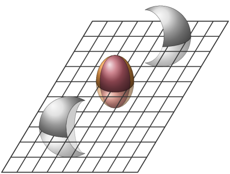
High energy heavy ion experiments have generated many surprising experimental observations which call for microscopic explanations. One is the degree of similarity between high multiplicity p+p collisions and A+A collisions. Another surprise is the extent to which the usual cartoons illustrating HICs, such as Fig. 1, involving smooth energy densities for the colliding nuclei are quite misleading. Instead, modern hydrodynamics codes typically start from initial conditions with extremely large fluctuations of energy and entropy density. (See figure 1 in Ref. Bernhard:2016tnd for a typical example.) These initial conditions are required to explain the large observed odd azimuthal flow moments, see e.g., Ref. Acharya:2018zuq . If odd moments solely arose from statistical fluctuations of the hydrodynamic fluid itself, then for symmetric collisions such as Pb+Pb, the odd flow coefficients , , etc., should be very significantly suppressed compared to the even coefficients , , etc., which is not the case. Here, as usual, the flow moments are defined by the azimuthal dependence of the produced particle distribution,
| (1) |
with the energy, momentum, transverse momentum, the azimuthal angle, the pseudorapidity of the particle, and the -th harmonic symmetry plane angle.
Hence typical AdS shock wave calculations involving smooth initial energy densities are too idealized. Even symmetric Pb+Pb collisions should be characterized by initial energy densities which are asymmetric owing to the presence of independent and substantial transverse variations. This was one of the motivations for our study Waeber:2019nqd of idealized but highly asymmetric planar shock collisions.
A further phenomenologically relevant aspect is that AdS/CFT models of collisions, in the leading infinite coupling limit, tend to predict surprisingly short hydrodynamization times and equilibration times222The here cited model treated in Balasubramanian:2010ce doesn’t sharply differentiate between hydrodynamization time and equilibration time. Here and henceforth we also use the term ”equilibration” synonymous with ”thermalization”., 0.3 fm/ or less Balasubramanian:2010ce . While there is no consensus among perturbative, i.e. weak coupling, estimates of the thermalization time scale , all estimates suggest it to be substantially longer. For example, an early result Baier:2000sb gave fm/, and a more recent result based on a different analysis Berges:2014yta is fm/. In Romatschke:2016hle it is argued from the perspective of hydrodynamics that thermalization might possibly never be reached in a realistic heavy-ion collision.
In our earlier work Waeber:2018bea using a specific resummation ansatz, we found that for realistic finite values of the ’t Hooft coupling of QCD, the imaginary part of the lowest QNM is roughly halved, corresponding to a doubling of the predicted equilibration time. In the present contribution we will argue that for fluctuations large enough to generate the observed values, the AdS prediction for the hydrodynamization time of individual transverse “pixels” are significantly lengthened but stay much smaller than found in perturbative calculations. However, we will also argue that complete thermalization could take much longer as it requires equilibration between these “pixels”.
Over the years many different hydrodynamics codes have been developed, improved and fine-tuned to describe the experimental data. Their relative advantages and disadvantages are the topic of specialized workshops. We do not want to enter this discussion here. Rather, we will focus on just one relatively recent study Bernhard:2016tnd which is especially systematic with respect to the properties we are interested in. We leave it to the authors of other studies to decide whether our conclusions are also relevant for their work.
In the following section we briefly review those results of Ref. Bernhard:2016tnd which are important for us and then discuss how these compare with the results of our AdS/CFT study Waeber:2019nqd . The present contribution was separated from Ref. Waeber:2019nqd because, unlike the well defined results of Ref. Waeber:2019nqd which should stand the test of time, the following discussion of phenomenological consequences depends crucially on the comparison of results from hydrodynamics codes to experimental data and is subject to far more uncertain interpretation. In particular, it is not yet feasible to perform numerical gravity calculations with initial conditions which fully mimic the strong transverse fluctuations of energy and entropy densities that appear to be present in real collisions.
In Section 3 we discuss implications for peripheral collisions and for p+A collisions. Section 4 is devoted to another aspect, namely the time dependence of the apparent horizon in asymmetric collisions and a comparison to what is known about the time dependence of entropy for classical and quantum gauge theories. A final section holds a few concluding remarks.
II The role of fluctuations in heavy ion collisions
The arguments in favor of strong fluctuations in the initial state of heavy ion collisions (HICs) are manifold, both theoretical and experimental. In, e.g., Ref. Muller:2011bb (see also Lappi:2017skr ) the initial fluctuations in transverse energy density were calculated in the Color Glass Condensate (CGC) model. It was argued that for typical pixels these can be larger than 50%. On the experimental side we have already noted the surprisingly large values observed, e.g., in Ref. Acharya:2018zuq .
Different models vary in their assumptions, including those which concern fluctuations. We will follow Ref. Bernhard:2016tnd whose Fig. 1 shows several typical examples of initial state fluctuations. The basic assumption of that paper, which we also adopt, is that one may think of the initial state of a HIC as arising from a sum over many isolated collisions of often vastly asymmetric “pixels”. Because these asymmetries are so large, holographic calculations for smooth symmetric shock wave collisions are insufficient.
Extending the AdS treatment to include realistic fluctuations is somewhat subtle because it relates to basic questions of what is exactly meant by “decoherence” and “thermalization.” While the fundamental T-invariance of QCD seems to imply the absence of any decoherence, this is no longer true if specific probes of only limited spatial extent are considered. All standard observables for high energy heavy-ion collisions do exactly that, probing only transverse scales which are much smaller than the nuclear radii, be it or, e.g., individual hadron radii. Therefore, real life heavy ion experiments always imply coarse graining, see again Fig. 1 of Bernhard:2016tnd , which circumvents this T-invariance argument. Basically, all experimental observables are insensitive to quantum correlations beyond the scales mentioned above.
The description of detailed properties of collisions of highly non-uniform nuclei by viscous relativistic hydrodynamics has been the topic of many careful and interesting investigations, far too many to review in this short note. Let us only mention Ref. Welsh:2016siu , where it was highlighted that the inclusion of realistic fluctuations is even more important if one studies collision systems like p+A. The fact that we limit our discussion here to Ref. Bernhard:2016tnd should not be interpreted as any form of judgment on the relative value of the various models but just as reflection of our inability to do justice to all of them.
One of the standard procedures, also adopted here, is to describe all collisions by means of a “nuclear thickness function” which is usually assumed to be a superposition of Gaussians of a certain width in the transverse plane. In Ref. Bernhard:2016tnd the randomly generated participant thickness function is constructed as follows:
| (2a) | |||||
| (2b) | |||||
where the coefficients are chosen according to the Gamma probability distribution,
| (3) |
with the parameter and the mean value of set to unity. The coefficients simulate the statistical fluctuations of the initial state, while are the random participant locations in the transverse plane. (See Ref. Bernhard:2016tnd for details.)
When we refer to “pixels” we mean independent transverse areas with a radius of order , where is the saturation scale of order 1–2 GeV in the initial state and not those areas with which hydrodynamics is initialized (with mean radius ), which we call “patches“ for distinction. The typical radius of a “pixel” is 0.1–0.2 fm, while that of a hydrodynamical “patch” is 0.4–1.2 fm, see table 1 in Ref. Moreland:2018gsh . However, in line with our comment above regarding the attractor properties of hydrodynamics, the initialization time for hydrodynamics can be chosen more or less at will in the range fm/ (see again Table 1 in Ref. Moreland:2018gsh ). In Ref. Bernhard:2016tnd the hydrodynamics code was actually initialized at fm/ which resulted in the fit value fm. This value for the patch size probably has little physical meaning, as hydrodynamics is definitely not applicable at fm/, but this is irrelevant for our discussion since the distribution is independent of and so are the resulting fluctuations. We will argue below that the relevant time scales for hydrodynamization and thermalization depend only on the distribution function .
The physical idea behind the thickness function is that due to length contraction and time dilation partons in the colliding nuclei are coherent in the longitudinal direction but incoherent in transverse distance beyond a characteristic length scale which is typically chosen as the inverse saturation scale fm. What is phenomenologically important is the assumption made about how the local initial entropy density (or related energy density) depends on the thickness functions of two colliding transverse pixels. Very little is known about this and models differ widely. The authors of Ref. Bernhard:2016tnd , therefore, use the flexible parameterisation
| (4) |
which covers a wide range of possibilities.
| (5) |
and simply vary the value of to find the one for which they obtain the best overall agreement with the data. This phenomenological analysis clearly favors the geometric mean (), see Fig. 9 of Ref. Bernhard:2016tnd , so that
| (6) |
This dependence of the initial entropy density on the geometric mean of the thickness functions is especially noteworthy in light of analogous results from studies of holographic collisions Waeber:2019nqd . This study found that in asymmetric collisions the rapidity dependence of the proper energy density of the produced plasma, near the onset of the hydrodynamic regime, is well described by the geometric mean of the produced proper energy densities in the corresponding symmetric collisions. Moreover, the hydrodynamization time hypersurface was found to be an almost perfect proper time hypersurface (i.e., the boundary of the hydrodynamic regime is essentially a hyperbola) whose value depends exclusively on the energy scale set by the geometric mean of the longitudinally integrated energy densities of the colliding pixels Waeber:2019nqd ; Chesler:2015fpa ,333Explicitly, , etc.
| (7) |
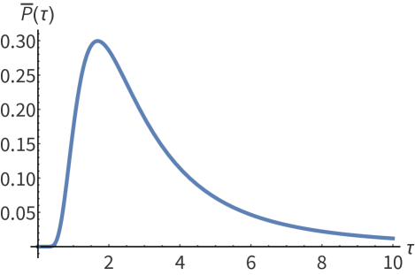
To connect this holographic result for hydrodynamization time to the model (6) of fluctuating initial conditions, we regard the energy scale of a given pixel of projectile as equal to the average scale times the fluctuating amplitude of some participant lying within this pixel, and likewise for projectile . One may then compute the resulting probability distribution of the hydrodynamization time . The result is
| (8) |
This distribution in plotted in Fig. 2. It is peaked at , a little below the value of which, from Eq. (7), would be the holographic prediction in the absence of fluctuations. Glancing at Fig. 2 and focusing on the peak in the distribution, one might think that the main effect of including initial state fluctuations is merely to induce relatively modest fluctuations in the hydrodynamization time so that it becomes, crudely, . This conclusion, however, is wrong due to the slow power-law decrease of the distribution with increasing time , which reflects the non-analytic behavior of the adopted form (3) of as .
The median of the distribution for is (for ), substantially larger than the peak value. The mean hydrodynamization time is given by
| (9a) | |||||
| (9b) | |||||
with the numeric value specific to , while the rms deviation is
| (10a) | |||||
| (10b) | |||||
considerably larger than the mean value. There is a 70% probability that the hydrodynamization time is larger than the non-fluctuating estimate of , a 45% probability that is larger than , and a 30% probability that it is larger than .
This simple model predicts that fluctuations in the transverse plane lead to large non-Gaussian fluctuations in the hydrodynamization time. For an individual collision of two pixels it doubles, on average, the hydrodynamization time, thereby converting the typical time scale of fm/ predicted by AdS/CFT modeling with smooth initial conditions Balasubramanian:2010ce to the range fm/. Moreover, it has consequences for thermalization of the complete nuclear system. Complete equilibration would require equilibration between different pixels. However, with significant variations in energy density and hence effective local temperature across the transverse extent of the fireball, such variations can only relax via hydrodynamic processes whose time scale grows linearly with the length scale of variations and exceeds the relevant initial hydrodynamization time. The fact that fluctuation are definitely not smoothed out at the initial hydrodynamization time explains why large fluctuations can still persist around 1 fm/ and generate a sizable triangular flow component . In other words, hadron phenomenology as encoded in hydrodynamics codes like Bernhard:2016tnd appears to be compatible with AdS/CFT modeling only because of large transverse fluctuations.
III Peripheral collisions
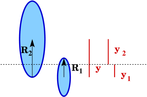
One original motivation for our investigation was the observation that, if hydrodynamization would occur significantly more slowly in the asymmetric fringe regions (the orange areas in Fig. 1) in peripheral collisions, then this would cause the hydrodynamized overlap region (the inner red region in Fig. 1) to be slimmer and thus increase . It turns out, however, that this effect is rather small and can be essentially neglected in comparison with the large fluctuation effects just discussed. To illustrate this, we consider in this section a very crude model that approximates the energy and entropy densities of each colliding nucleus as homogeneous within its Lorentz contracted spherical volume, such that the asymmetry for a given pixel is exclusively determined by geometry. The nuclei move in the direction and the reaction plane is the plane. The transverse energy densities at a given transverse position indicated by the dashed line in Fig. 3 are then given by
| (11) |
where are the two nucleon numbers, the two nuclear radii, the Lorentz factors of each nucleus, and the transverse distances from the centers of the nuclei in reaction plane and orthogonal to it. We defined . Finally, is the impact parameter.
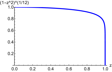
The resulting geometric mean of the scale parameter is
| (12) |
As shown in Fig. 4, this function goes to zero as , or , so abruptly that the impact on is negligible.
Let us add that it follows also from the geometric mean of the energy scales that the difference between smooth and smooth collisions, i.e., neglecting effects due to fluctuations, is not dramatic. For the momentum scale is smaller by a factor compared to and thus the hydrodynamization time is larger by that factor 2.5 (for Pb) increasing fm/ to fm/. Thus, also in this case, fluctuations have the strongest impact on the hydrodynamization time, implying that and collisions should have similar properties because, in a holographic description, the essential difference of incident nucleons versus nuclei is solely encoded in their respective energy densities. We mention in passing that in Ref. Waeber:2019nqd it was found that in forward direction of the heavier nucleus in a asymmetric collision the matter density is larger and thus hydrodynamization happens slightly earlier.
IV Entropy production in classical and quantum gauge theories
It is possible to extend the motivation for the present contribution to a grander scale. Decoherence, entropy production and hydrodynamization or thermalization are intensely discussed also in other fields like quantum gravity and quantum computing. AdS/CFT duality has the potential to connect all of these fields. It was established in recent years that there exists an intimate connection to quantum error correction schemes while by construction AdS/CFT combines quantum gravity and quantum field theory.
In principle, the connection to QCD and HICs opens the very attractive possibility for experimental tests of theoretical predictions because the number of final state hadrons per rapidity interval is taken as a measure of thermodynamic entropy in the final state after all interactions have stopped. Obviously this is, however, only helpful if the differences between CFT and QCD are minor.
As entropy production is equivalent to information loss, this discussion centers on the question in which sense information can get lost under unitary time evolution and how this potential information loss in the boundary theory is related to the generation of the Bekenstein-Hawking entropy of the formed large black branes in the (AdSS5) bulk.
There exists a fundamental difference with respect to ergodic properties in the relation between (AdSS5)/CFT and QCD for high and low temperature, which is most obvious from the fact that (AdSS5)/CFT is conformal and QCD below the confinement-deconfinement transition temperature is not. However, there are strong indications that far above this pseudocritical temperature the classical solutions of Einstein’s equation on the AdS side produce results that match perfectly relativistic hydrodynamics which, in turn, provides a near-perfect description of the experimentally observed properties of the high energy phase of HICs, see e.g. vanderSchee:2013pia . Also, it was shown that on the string theory side the leading quantum corrections are not large Buchel:2008ac ; Buchel:2008sh ; Stricker:2013lma ; Waeber:2018bea . The latter appears to be a general trend. In principle, classical chaos and quantum chaos can differ fundamentally but it seems that for the high temperature phase of QCD they do not.
Here we want to address only one aspect of this extensive discussion to which our calculations may add some insight. For classical ergodic theories the coarse-grained entropy grows linearly in time with a rate given by the Kolmogorov-Sinai entropy defined as the sum of all positive Lyapunov exponents :
| (13) |
Because the definition of entropy is ambiguous in a non-equilibrium setting one can ask the question: “For which definition of entropy in the quantum theory does one observe linear growth with boundary time?”. We will not address the much deeper question whether the condition of linear growth is required or at least well motivated.
Quantum chaos can be described quantitatively in terms of exponential growth of out-of-time-order correlators (OTOCs)444 As pointed out by the authors of Rozenbaum_2019 , the identification of the exponential growth of OTOCs with Lyapunov exponents depends on the specific choice of initial states. The general relation between the growth rate of OTOCs and classical Lyapunov exponents is both nontrivial and so far not fully understood.
| (14) |
of suitable operators , Larkin ; Almheiri:2013hfa ; Maldacena:2015waa , where in the semi-classical limit should be close to the largest classical Lyapunov exponent. For many models this behavior was indeed established. For example in Ref. Stanford:2015owe it was found for a weakly coupled matrix theory that
| (15) |
with the ′t Hooft parameter . Kitaev kitaev found for a setting similar to the Sachdev-Ye model sachdev that the Maldacena-Shenker-Stanford (MSS) bound Maldacena:2015waa gets saturated for infinite coupling strength:
| (16) |
In Buividovich:2018scl the BFSS matrix model was investigated numerically and it was found, as in all other investigations known to us, that the leading exponent for a quantum theory stays below the MSS bound, often even substantially so.
It is indisputable that classical Yang-Mills theories show classical chaotic behavior, i.e. after an initial phase, which depends on the chosen initial conditions, a period of linear growth of the coarse-grained entropy sets in, followed by saturation at the thermal equilibrium value. Numerical studies of classical Yang-Mills theories showing this behavior can be found, e.g., in Ref. Muller:1992iw ; Biro:1994bi ; Bolte:1999th ; Iida:2013qwa . In Biro:1994sh it was conjectured that the largest Lyapunov exponent in a lattice discretized classical SU(N) Yang-Mills theory at weak coupling is given by
| (17) |
based on numerical simulations for Muller:1992iw ; Gong:1992yu . In Kunihiro:2010tg phenomenological arguments were given that for real QCD at the ′t Hooft coupling relevant to the early stage of a HIC, the largest Lyapunov exponent is of the order
| (18) |
significantly below the MSS bound.
There exist many more publications worth mentioning in this context. A very recent example dealing with QCD is, e.g., Akutagawa:2019awh , while in Ref. Bianchi:2017kgb it is argued that, at least for entanglement entropy, bosons, and a quadratic Hamiltonian, a linear growth of entropy with the Kolmogorov-Sinaï entropy can be derived also for quantum systems. Using the coarse graining approach of Husimi distributions, the authors of Ref. Kunihiro:2008gv argued that the growth rate of the coarse-grained Wehrl entropy of a quantum system is equal to the Kolmogorov-Sinaï entropy of its classical counterpart.
Numerical AdSS5 calculations confirm this picture and add a specific angle. Here, the classical Einstein equation is solved on AdS space-time for boundary conditions that mimic, e.g., HICs Chesler:2008hg ; Chesler:2010bi ; Chesler:2013lia ; Chesler:2015wra . In this setting the size of the apparent horizon is the appropriate measure for the produced entropy (see e.g. Engelhardt:2017aux ). We will elaborate on this point in more detail below.555The event horizon is not suitable as it depends on the entire future history. Fig. 3 in Ref. Chesler:2008hg shows for a specific setting that the apparent horizon grows linearly with time for an appreciable period, just as expected.
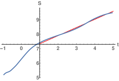
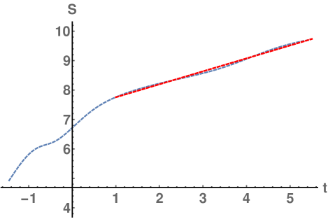
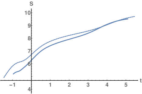
Shock wave collisions in SYM theory, which can be computed via their gravitational dual description in AdS5, are believed to behave in many qualitative aspects very similar to HICs. The AdS/CFT duality links the volume element of the apparent horizon to the entropy density666Strictly speaking this relation is only valid in the equilibrium case. As in e.g. Wilke_da ; Grozdanov:2016zjj we exploit this relation also off-equilibrium and use it to define the entropy(-density) in this case. In general the dictionary giving an interpretation of geometric objects in Anti-de Sitter space in terms of the boundary field theory is far from being complete and remains elusive for many cases, see e.g. Engelhardt:2017wgc times an infinitesimal spatial boundary volume . Using this relation, the longitudinally integrated entropy density in symmetric collisions in five dimensional AdS space was calculated, e.g., in Ref. Grozdanov:2016zjj (see dashed curves of Fig. 5 in Grozdanov:2016zjj ). Our results for the entropy production (longitudinally integrated, given in units of ) during symmetric collisions are discussed in Fig. 5. They are seen to correspond closely to the findings in Grozdanov:2016zjj . In Fig. 6 and Fig. 7 we compare this to the analogous computation during asymmetric collisions. The code used in this calculation is described in detail in Ref. Waeber:2019nqd .
For large enough times the growth of the area of the apparent horizon is close to linear, as expected, with a slight superimposed oscillation which probably averages out over sufficiently long time periods.777The small wiggling around linear growth seen in Figs. 5 and 6 can be explained by damped oscillations induced by the lowest quasinormal mode and can thus be expected to fade off for larger times. The observation that the rate of growth of the apparent horizon area is almost identical for the two cases shown in Figs. 5 and 6 is relevant for the physics of HICs because the longitudinal thickness of both ions in the overlap region is very asymmetric in some regions of the transverse plane. However, the gradient of the linear growth should be independent of these initial conditions.
Thus, at large times linear entropy growth does not only seem to connect classical and quantum chaos for QFTs but also their holographic dual description. Obviously, these similarities could well be accidental at our present stage of understanding, but they are sufficiently intriguing to warrant further research.
V Conclusion
In this note we have argued that detailed holographic calculations for asymmetric collisions are highly relevant for any quantitative description of realistic HICs. We have performed such calculations and have found that:
-
•
The characteristic large fluctuations in transverse energy and entropy densities, which are required in hydrodynamic descriptions to explain the observed large event-by-event fluctuations of flow observables, delay hydrodynamization and equilibration in the holographic description so strongly that they are still significant at time of 1–2 fm/ when hydrodynamics becomes definitively applicable.
-
•
In contrast, the effect of the transverse dependence of energy densities in peripheral collisions has only a minor impact on the hydrodynamization time, such that it is well motivated to initialize hydrodynamics for the entire system simultaneously.
-
•
p+A and A+A collisions do not show major differences in hydrodynamization properties.
-
•
The long time linear growth of the apparent horizon is very similar for symmetric and asymmetric collisions which supports its interpretation as entropy.
Finally, it should be noted that while the delayed hydrodynamization and equilibration caused by initial state fluctuations is helpful to explain the observed fluctuations it also increases concerns that thermalization might not happen as rapidly as is usually assumed in the interpretation of the medium modifications of “hard” probes.
Acknowledgements
BM acknowledges support from the U.S. Department of Energy grant DE-FG02-05ER41367. LY acknowledges support from the U.S. Department of Energy grant DE-SC0011637. SW acknowledges support from the Elite Network of Bavaria in form of a Research Scholarship grant. AS and SW acknowledge support by BMBF (Verbundprojekt 05P2018, 05P18WRCA1).
References
- (1) S. Waeber, A. Rabenstein, A. Schäfer and L. G. Yaffe, “Asymmetric shockwave collisions in ,” JHEP 1908 (2019) 005 [arXiv:1906.05086].
- (2) P. M. Chesler, N. Kilbertus and W. van der Schee, “Universal hydrodynamic flow in holographic planar shock collisions,” JHEP 1511 (2015) 135 [arXiv:1507.02548].
- (3) W. van der Schee, P. Romatschke and S. Pratt, “Fully Dynamical Simulation of Central Nuclear Collisions,” Phys. Rev. Lett. 111 (2013) 222302, [arXiv:1307.2539].
- (4) S. Waeber and A. Schäfer, “Studying a charged quark gluon plasma via holography and higher derivative corrections,” JHEP 1807 (2018) 069 [arXiv:1804.01912].
- (5) A. Buchel, “Shear viscosity of boost invariant plasma at finite coupling,” Nucl. Phys. B 802 (2008) 281 [arXiv:0801.4421].
- (6) A. Buchel, “Resolving disagreement for eta/s in a CFT plasma at finite coupling,” Nucl. Phys. B 803 (2008) 166 [arXiv:0805.2683].
- (7) S. A. Stricker, “Holographic thermalization in N=4 Super Yang-Mills theory at finite coupling,” Eur. Phys. J. C 74 (2014) no.2, 2727 [arXiv:1307.2736].
- (8) G. Endrodi, M. Kaminski, A. Schäfer, J. Wu and L. Yaffe, “Universal Magnetoresponse in QCD and SYM,” JHEP 1809 (2018) 070 [arXiv:1806.09632].
- (9) M. Panero, “Thermodynamics of the QCD plasma and the large-N limit,” Phys. Rev. Lett. 103 (2009) 232001 [arXiv:0907.3719].
- (10) G. S. Bali, F. Bursa, L. Castagnini, S. Collins, L. Del Debbio, B. Lucini and M. Panero, “Mesons in large-N QCD,” JHEP 1306 (2013) 071 [arXiv:1304.4437].
- (11) J. Berges, K. Boguslavski, S. Schlichting and R. Venugopalan, “Universal attractor in a highly occupied non-Abelian plasma,” Phys. Rev. D 89 (2014) 1140077 [arXiv:1311.3005].
- (12) P. Romatschke, “Relativistic Fluid Dynamics Far From Local Equilibrium,” Phys. Rev. Lett. 120 (2018) 012301 [arXiv:1704.08699].
- (13) P. Romatschke, “Relativistic Hydrodynamic Attractors with Broken Symmetries: Non-Conformal and Non-Homogeneous,” JHEP 1712 (2017) 079 [arXiv:1710.03234].
- (14) J. E. Bernhard, J. S. Moreland, S. A. Bass, J. Liu and U. Heinz, “Applying Bayesian parameter estimation to relativistic heavy-ion collisions: simultaneous characterization of the initial state and quark-gluon plasma medium,” Phys. Rev. C 94 (2016) no.2, 024907 [arXiv:1605.03954 [nucl-th]].
- (15) S. Acharya et al. [ALICE Collaboration], “Anisotropic flow of identified particles in Pb-Pb collisions at TeV,” JHEP 1809 (2018) 006 [arXiv:1805.04390].
- (16) V. Balasubramanian et al., “Thermalization of Strongly Coupled Field Theories,” Phys. Rev. Lett. 106 (2011) 191601 [arXiv:1012.4753].
- (17) R. Baier, A. H. Mueller, D. Schiff and D. T. Son, “’Bottom up’ thermalization in heavy ion collisions,” Phys. Lett. B 502 (2001) 51 [hep-ph/0009237].
- (18) J. Berges, B. Schenke, S. Schlichting and R. Venugopalan, “Turbulent thermalization process in high-energy heavy-ion collisions,” Nucl. Phys. A 931 (2014) 348 [arXiv:1409.1638].
- (19) P. Romatschke, “Do nuclear collisions create a locally equilibrated quark-gluon plasma?,” Eur. Phys. J. C 77 (2017) no.1, 21 [arXiv:1609.02820].
- (20) B. Müller and A. Schäfer, “Transverse Energy Density Fluctuations in Heavy-Ion Collisions in a Gaussian Model,” Phys. Rev. D 85 (2012) 114030 Erratum: [Phys. Rev. D 96 (2017) no.5, 059903] [arXiv:1111.3347].
- (21) T. Lappi and S. Schlichting, “Linearly polarized gluons and axial charge fluctuations in the Glasma,” Phys. Rev. D 97 (2018) no.3, 034034 [arXiv:1708.08625].
- (22) K. Welsh, J. Singer and U. W. Heinz, “Initial state fluctuations in collisions between light and heavy ions,” Phys. Rev. C 94 (2016) no.2, 024919 [arXiv:1605.09418].
- (23) J. S. Moreland, J. E. Bernhard and S. A. Bass, “Estimating initial state and quark-gluon plasma medium properties using a hybrid model with nucleon substructure calibrated to -Pb and Pb-Pb collisions at TeV,” [arXiv:1808.02106].
- (24) A.I. Larkin and Y.N. Ovchinnikov, “Nonuniform state of superconductors,” Sov.Phys.JETP 20 (1965) 762
- (25) A. Almheiri, D. Marolf, J. Polchinski, D. Stanford and J. Sully, “An Apologia for Firewalls,” JHEP 1309 (2013) 018 [arXiv:1304.6483].
- (26) J. Maldacena, S. H. Shenker and D. Stanford, “A bound on chaos,” JHEP 1608 (2016) 106 [arXiv:1503.01409].
- (27) D. Stanford, “Many-body chaos at weak coupling,” JHEP 1610 (2016) 009 [arXiv:1512.07687].
-
(28)
A. Kitaev, talks at KITP
http://online.kitp.ucsb.edu/online/entangled15/kitaev/,
http://online.kitp.ucsb.edu/online/entangled15/kitaev2/, April and May, 2015 - (29) S. Sachdev and J. Ye, “Gapless spin fluid ground state in a random, quantum Heisenberg magnet,” Phys. Rev. Lett. 70 (1993) 3339, [cond-mat/9212030].
- (30) P. V. Buividovich, M. Hanada and A. Schäfer, “Quantum chaos, thermalization, and entanglement generation in real-time simulations of the Banks-Fischler-Shenker- Susskind matrix model,” Phys. Rev. D 99 (2019) no.4, 046011 [arXiv:1810.03378].
- (31) B. Müller and A. Trayanov, “Deterministic chaos in nonAbelian lattice gauge theory,” Phys. Rev. Lett. 68 (1992) 3387.
- (32) T. S. Biro, S. G. Matinyan and B. Müller, “Chaos and gauge field theory,” World Sci. Lect. Notes Phys. 56 (1994) 1.
- (33) J. Bolte, B. Müller and A. Schäfer, “Ergodic properties of classical SU(2) lattice gauge theory,” Phys. Rev. D 61 (2000) 054506 [hep-lat/9906037].
- (34) H. Iida, T. Kunihiro, B. Müller, A. Ohnishi, A. Schäfer and T. T. Takahashi, “Entropy production in classical Yang-Mills theory from Glasma initial conditions,” Phys. Rev. D 88 (2013) 094006 [arXiv:1304.1807].
- (35) T. S. Biro, C. Gong and B. Müller, “Lyapunov exponent and plasmon damping rate in nonabelian gauge theories,” Phys. Rev. D 52 (1995) 1260 [hep-ph/9409392].
- (36) C. Q. Gong, “Lyapunov exponent of classical SU(3) gauge theory,” Phys. Lett. B 298 (1993) 257 [hep-lat/9209018].
- (37) T. Kunihiro, B. Müller, A. Ohnishi, A. Schäfer, T. T. Takahashi and A. Yamamoto, “Chaotic behavior in classical Yang-Mills dynamics,” Phys. Rev. D 82 (2010) 114015 [arXiv:1008.1156].
- (38) T. Akutagawa, K. Hashimoto, K. Murata and T. Ota, “Chaos of QCD string from holography,” [arXiv:1903.04718].
- (39) E. Bianchi, L. Hackl and N. Yokomizo, “Linear growth of the entanglement entropy and the Kolmogorov-Sinai rate,” JHEP 1803 (2018) 025 [arXiv:1709.00427].
- (40) T. Kunihiro, B. Müller, A. Ohnishi and A. Schafer, “Towards a Theory of Entropy Production in the Little and Big Bang,” Prog. Theor. Phys. 121, 555 (2009) [arXiv:0809.4831 [hep-ph]].
- (41) P. M. Chesler and L. G. Yaffe, “Horizon formation and far-from-equilibrium isotropization in supersymmetric Yang-Mills plasma,” Phys. Rev. Lett. 102 (2009) 211601 [arXiv:0812.2053].
- (42) P. M. Chesler and L. G. Yaffe, “Holography and colliding gravitational shock waves in asymptotically spacetime,” Phys. Rev. Lett. 106 (2011) 021601 [arXiv:1011.3562].
- (43) P. M. Chesler and L. G. Yaffe, “Numerical solution of gravitational dynamics in asymptotically anti-de Sitter spacetimes,” JHEP 1407 (2014) 086 [arXiv:1309.1439].
- (44) P. M. Chesler and L. G. Yaffe, “Holography and off-center collisions of localized shock waves,” JHEP 1510 (2015) 070 [arXiv:1501.04644].
- (45) W. van der Schee, Gravitational collisions and the quark-gluon plasma, [arXiv:1407.1849].
- (46) N. Engelhardt and A. C. Wall, “Decoding the Apparent Horizon: Coarse-Grained Holographic Entropy,” Phys. Rev. Lett. 121 (2018) no.21, 211301 [arXiv:1706.02038].
- (47) N. Engelhardt and A. C. Wall, “No Simple Dual to the Causal Holographic Information?,” JHEP 1704 (2017) 134 [arXiv:1702.01748 [hep-th]].
- (48) S. Grozdanov and W. van der Schee, “Coupling Constant Corrections in a Holographic Model of Heavy Ion Collisions,” Phys. Rev. Lett. 119 (2017) no.1, 011601 [arXiv:1610.08976].
- (49) H. M. Tsai and B. Müller, “Entropy production and equilibration in Yang-Mills quantum mechanics,” Phys. Rev. E 85 (2012) 011110 [arXiv:1011.3508].
- (50) E. B. Rozenbaum, S. Ganeshan, V. Galitski “Universal level statistics of the out-of-time-ordered operator,” Phys. Rev. B 100 (2019) 035112 [arXiv:1801.10591].