Chemical abundances of Seyfert 2 AGNs– II. $N2$ metallicity calibration based on SDSS

Abstract

We present a semi-empirical calibration between the metallicity ($Z$) of Seyfert 2 Active Galactic Nuclei and the $N2$=log([N ii]$\lambda$6584/H$\alpha$) emission-line intensity ratio. This calibration was derived through the [O iii]$\lambda$5007/[O ii]$\lambda$3727 versus $N2$ diagram containing observational data and photoionization model results obtained with the Cloudy code. The observational sample consists of 463 confirmed Seyfert 2 nuclei (redshift $z\>\la 0.4$) taken from the Sloan Digital Sky Survey DR7 dataset. The obtained $Z$-$N2$ relation is valid for the range $0.3\>\la\>(Z/Z_{\odot})\>\la\>2.0$ which corresponds to $-0.7\>\la\>(N2)\>\la\>0.6$. The effects of varying the ionization parameter ($U$), electron density and the slope of the spectral energy distribution on the $Z$ estimations are of the order of the uncertainty produced by the error measurements of $N2$. This result indicates the large reliability of our $Z-N2$ calibration. A relation between $U$ and the [O iii]/[O ii] line ratio, almost independent of other nebular parameter, was obtained.

1 Introduction

Active Galactic Nuclei (AGNs) are the most luminous objects in the Universe and present strong emission-lines in their spectra. The metallicity derived through these emission-lines offers a very powerful tool for understanding the chemical galaxy evolution along the Hubble time.

Among the heavy elements present in the gas phase of gaseous nebulae, oxygen is the element most widely used as a proxy for global gas-phase metallicity $Z$ (e.g. Kennicutt et al. 2003; Hägele et al. 2008; Yates et al. 2012) because prominent emission lines from their main ionic stages are present in the optical spectra of these objects. It is consensus that bona fide oxygen abundance determinations in star-forming regions and planetary nebulae are those based on direct detection of the electron temperature ($T_{\rm e}$) of the gas, the so-called $T_{\rm e}$-method. The agreement between oxygen abundances in the gas phase of H ii regions with those derived through observations of the weak interstellar O i$\lambda$1356 line towards the stars located at similar galactocentric distance in the Milky Way (Pilyugin, 2003) indicates the $T_{\rm e}$-method is consistent with other more precise ways of deriving the metallicity. However, this method requires the measurement of certain weak emission-lines sensitive to $T_{\rm e}$, such as [O iii]$\lambda$4363 ($\sim$100 times weaker than H$\beta$), which makes $T_{\rm e}$-method only applied to objects with high ionization degree and/or low metallicity (e.g. Smith 1975; Castellanos et al. 2002; Kennicutt et al. 2003; Izotov et al. 2006; Hägele et al. 2008; Sanders et al. 2016, 2019, among others). In the cases where the $T_{\rm e}$-method can not be applied, theoretical or (semi-) empirical calibrations between abundances or metallicity and more easily measurable line ratios can be used instead, the so-called strong-line method (for a review, see Pérez-Montero 2017; Peimbert, Peimbert, & Delgado-Inglada 2017; Kewley et al. 2019; Maiolino & Mannucci 2019; Garcia-Rojas 2020).

In regarding AGNs, the $T_{\rm e}$-method tends to underestimate the oxygen abundance by an average value of about 0.6 dex in comparison to estimations based on strong-line methods and it produces subsolar O/H values for most of these objects (Dors et al., 2015, 2020). An alternative method to derive the metallicity or abundances in the nuclear regions of spiral galaxies is the extrapolation of the radial oxygen abundance. Along decades, results based on this indirect method have indicated $Z$ near or slightly above the solar value in nuclear regions (Vila-Costas & Edmunds, 1992; Zaritsky et al., 1994; van Zee et al., 1998; Pilyugin et al., 2004; Gusev et al., 2012; Dors et al., 2015; Zinchenko et al., 2019), in consonance with predictions of chemical evolution models (e.g. Mólla & Díaz 2005) and with the use of strong-line methods (e.g. Groves et al. 2004, 2006; Feltre, Charlot & Gutkin 2016; Thomas et al. 2019; Pérez-Montero et al. 2019; Dors et al. 2020). Therefore, $T_{\rm e}$-method does not seem to work for AGNs. The origin of the discrepancy between $Z$ values calculated via $T_{\rm e}$-method and via strong-line methods, the so-called $T_{\rm e}$-problem, could be attributed, in part, to the presence of heating/ionization by gas shock in the Narrow Line Region (NLR) of AGNs. In fact, Contini (2017) carried out detailed modelling of AGN optical emission-lines by using the SUMA code (Contini & Aldrovandi, 1983) and suggested the presence of gas shock with low velocity ($v\>\la\>400\>\rm km\>s^{-1}$) in a sample of Seyfert 2 nuclei. This result is supported by recent spatially resolved observational studies of Seyfert 2 nuclei, in which the presence of gas outflows with velocity of the order of 100-300 $\rm km\>s^{-1}$ have been found (e.g. Riffel et al. 2017, 2018). Moreover, the $T_{\rm e}$-problem can also be originated due to the use of an unappropriate calculation of the Ionization Correction Factor (ICF) for oxygen in AGNs (Pérez-Montero et al., 2019; Dors et al., 2020).

The most common way to obtain a calibration between strong emission-lines and $Z$ (or O/H) is through the use of photoionization models. The basic idea is to calculate emission-line ratios sensitive to $Z$ taking into account their dependence on other nebular parameters such as, the ionization parameter ($U$) of the gas, electron density, among others. For the optical range, the first calibration based on photoionization models for AGNs was proposed by Storchi-Bergmann et al. (1998), who used the line ratios [N ii]$\lambda$$\lambda$6548,6594/H$\alpha$, [O iii]$\lambda$$\lambda$4949,5007/H$\beta$ and [O ii]$\lambda$$\lambda$3726,3729/[O iii]$\lambda$$\lambda$4949,5007. In this case, [N ii]/H$\alpha$ is the $Z$ indicator, as proposed by Storchi-Bergmann et al. (1994), and the ratios involving [O iii] are mainly dependent on the ionization degree rather than $Z$. Most recently, Castro et al. (2017), using a comparison between photoionization models results and heterogeneous observational data of 58 Seyfert 2 nuclei, proposed a semi-empirical calibration of $Z$ with the $N2O2$=[N ii]$\lambda$6584/[O ii]$\lambda$3727 index. Throughout the paper, [O ii]$\lambda$3727 refers to the sum of [O ii]$\lambda$3726 and [O ii]$\lambda$3729.

The $N2O2$ line ratio presents some advantages over other $Z$ indicators. Firstly, $N2O2$ is not bi-valued as the most widely used $R_{23}$=([O ii]$\lambda$3727+[O iii]$\lambda$$\lambda$4949,5007)/H$\beta$ index, proposed by Pagel et al. (1979) and usually used in H ii region studies. Thus, the $N2O2$ estimates metallicities in a wide range of $Z$ values ($0.5\>\la\>(Z/Z_{\odot})\>\la\>2.0$; Castro et al. 2017). Secondly, $N2O2$ involves ions with similar ionization potentials, which minimizes the effects of the presence of possible secondary heating (ionizing) sources. However, $N2O2$ suffers some limitations, mainly because it requires spectrophotometric data covering a wide spectral range, making the reddening correction crucial. Moreover, in recent optical surveys, e.g. MaNGA (Mapping Nearby Galaxies at the Apache Point Observatory, Law et al. 2015), the [O ii]$\lambda$3727 line is measured in very few objects (e.g. Rembold et al. 2017; do Nascimento et al. 2019). Even in the data from the Sloan Digital Sky Survey (SDSS, York et al. 2000), when the presence of the [O ii]$\lambda$3727 line is considered in the selection criteria of objects, the sample is considerably reduced (e.g. Pilyugin & Mattsson 2011). In this sense, the $N2$=log([N ii]$\lambda$6584/H$\alpha$) seems to be a better $Z$ indicator than $N2O2$.

In this paper, the observational data of confirmed Seyfert 2 AGNs, taken from the Sloan Digital Sky Survey (SDSS, York et al. 2000) DR7 and selected by Dors et al. (2020), hereafter referred as Paper I, were combined with photoionization model results in order to explore the feasibility of the [N ii]$\lambda$6584/H$\alpha$ ratio as a metallicity indicator. This paper is organized as follows: In Section 2, a description of the methodology used to obtain the $Z-N2$ calibration is presented. In Sect. 3, a comparison between the observational data and photoionization model results as well as the calibration obtained are presented. The discussion is presented in Sect. 4. In Sect. 5, the summary and the conclusions of the outcome are presented.

2 Methodology

To obtain a calibration between the $Z$ and the $N2$ index, the same methodology used by Castro et al. (2017) and Dors et al. (2019) to calibrate the $Z$ with optical and ultraviolet NLRs associated to type-2 AGNs, respectively, was adopted. Based on the [O iii]$\lambda$5007/[O ii]$\lambda$3727 versus [N ii]$\lambda$6584/H$\alpha$ diagram, the observational data of Seyfert 2 AGNs were compared with photoionization model predictions. From this diagram, for each object, the metallicity and the corresponding $N2$ value were obtained, resulting in an unidimensional calibration. In what follows, descriptions of the observational sample and of the photoionization models are presented.

2.1 Observational data

We used optical emission-line intensities of Seyfert 2 nuclei taken from the Sloan Digital Sky Survey (SDSS, Abazajian et al. 2009) DR7 presented in Paper I. These data comprehend reddening corrected intensities (in relation to H$\beta$) of the [O ii]$\lambda$3726+$\lambda$3729, [Ne iii]$\lambda$3869, [O iii]$\lambda$4363, [O iii]$\lambda$5007, He I$\lambda$5876, [O i]$\lambda$6300, H$\alpha$, [N ii]$\lambda$6584, [S ii]$\lambda$6716, [S ii]$\lambda$6731 and [Ar iii]$\lambda$7135 emission-lines. The line measurements were carried out by the MPA/JHU group.

Observational data taken from the SDSS have been widely used to derive physical properties of AGNs (e.g. Vaona et al. 2012; Zhang et al. 2013). However, in most cases, the classification of AGN-like objects has been obtained by using only standard Baldwin-Phillips-Terlevich diagrams (Baldwin et al., 1981; Veilleux & Osterbrock, 1987), which include, for instance, Seyfert 1s, Seyfert 2s, quasars, H ii-like objects with very strong winds and gas shocks. Therefore, with the goal of selecting only Seyfert 2 objects, in the Paper I, we used a set of diagnostic diagrams to select AGN-like objects. Subsequently, the resulting data sample were compared with their classification obtained from the NED/IPAC (NASA/IPAC Extragalactic Database) database in order to select only objects classified as Seyfert 2 nuclei. This procedure resulted in a sample of 463 Seyfert 2 nuclei with redshifts $z\>\la\>0.4$ and with stellar masses of the hosting galaxies (also taken from the MPA-JHU group) in the range of $9.4\>\la\>\log(M/\rm M_{\odot})\>\la\>11.6$. From the compiled sample, we selected the intensities of the [O ii]$\lambda 3727$, [O iii]$\lambda 5007$, H$\alpha$, and [N ii]$\lambda 6584$ emission-lines relative to H$\beta$. The reader is referred to Paper I for a complete description about the observational data and aperture effects on $Z$ estimation.

2.2 Photoionization models

We considered version 17.00 of the Cloudy code (Ferland et al., 2017) in order to build up photoionization model grids assuming a wide range of nebular parameters. These models are similar to the ones considered by Dors et al. (2019) and the reader is referred to this paper for a complete description. The input parameters are described below.

1. SED: The Spectral Energy Distribution (SED) was assumed to be composed of the sum of two components: one representing the Big Blue Bump peaking at $\rm 1\>Ryd$, and the other a power law with spectral index $\alpha_{x}=-1$ representing the non-thermal X-ray radiation. The continuum between 2 keV and 2500Å is described by a power law with a spectral index $\alpha_{ox}$, for which we consider three different values: $-$0.8, $-$1.1 and $-1.4$, i.e. about the range of values estimated for Seyfert 2 and Quasars (e.g. Ho 1999; Miller et al. 2011; Zhu et al. 2019). It must be noted that models assuming $\alpha_{ox}\><\>-1.4$ predict very low emission-line intensities (relative to H$\beta$), when compared to those from our observational data (see also Dors et al. 2012). Moreover, observational estimations of $\alpha_{ox}$ have shown that few AGNs present $\alpha_{ox}$ out of this range of values (see Figure 1 of Dors et al. 2019).

2. Metallicity: The values of metallicity in relation to the solar one ($Z/Z_{\odot}$)= 0.2, 0.5, 0.75, 1.0, 1.5, and 2.0, were assumed in the models. Assuming the solar oxygen abundance $\rm 12+\log(O/H)_{\odot}=8.69$ (Asplund et al., 2009; Alende Prieto et al., 2001), the $Z$ values above corresponding to 12+log(O/H)= 8.0, 8.40, 8,56, 8.69, 8.86, 9.00, respectively, Metallicity values in this range has been found for AGNs with redshifts varying from $\sim 0$ to $\sim 7$ (e.g. Nagao et al. 2006a; Feltre, Charlot & Gutkin 2016; Matsuoka et al. 2018; Thomas et al. 2019; Mignoli et al. 2019; Pérez-Montero et al. 2019; Dors et al. 2014, 2015, 2018). We found that photoionization models assuming ($Z/Z_{\odot})\>>\>2.0$ produce similar intensities of $N2$, therefore, only $(Z/Z_{\odot})\>\lid\>2.0$ were assumed in our analysis. The abundance of all heavy elements was linearly scaled with $Z$, with the exception of the nitrogen abundance, which was calculated by using the following relation

   $$\rm\log(N/O)=1.29\>\times\>12+\log(O/H)\>-\>11.84,$$ (1)

   valid for $\rm 12+\log(O/H)\>\ga\>8.0$ or $(Z/Z_{\odot})\>\ga\>0.2$. This relation was obtained fitting N and O abundance estimations derived using detailed photoionization models by Dors et al. (2017) for a sample of Seyfert 2 AGNs located at $z\><\>0.1$ and also taking abundance estimations for H ii regions into account. The considered H ii regions are located in irregular and spiral local galaxies and the oxygen abundance estimations were obtained by Pilyugin & Grebel (2016) using the C method (Pilyugin et al., 2012). In Figure 1, abundance estimations and the fit represented by the Equation 1 are shown.

   

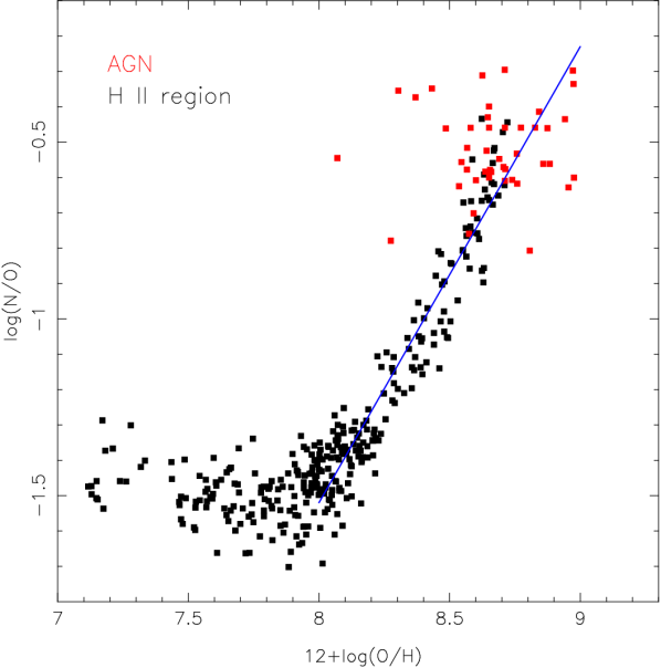
   Figure 1: log(N/O) versus 12+log(O/H) abundance ratio values. Red points are values predicted by the individual photoionization models for a sample of Seyfert 2 nuclei by Dors et al. (2017). Black points are estimations for H ii regions derived by Pilyugin & Grebel (2016) through the C method (Pilyugin et al., 2012). The line represents a linear regression [for $\rm 12+\log(O/H)\>\ga\>8.0$] fitting to the points and represented by Equation 1.

   It is worth to mention that the nitrogen and oxygen abundance relation changes with the cosmic time (redshift) and any calibration between $Z$ and nitrogen emission-lines must take into account the influence of this chemical evolution. In fact, Vincenzo & Kobayashi (2018) analysed the evolution of the (N/O)-(O/H) relation with the redshift making use of cosmological hydrodynamical simulations including detailed chemical enrichment. These authors found that higher N/O abundance ratios for a given O/H value are derived for low redshift ($z\>\la\>1$) in comparison with those having very high redshift ($z\>\ga\>5$, see Fig. 7 of their work). However, the study carried out by Vincenzo & Kobayashi (2018) is based on star-forming regions modelling and, apparently, an opposite result is derived for AGN-like objects (Dors et al., 2019). Moreover, the (N/O)-(O/H) relation for star-forming regios can also change in cases where these objects are located in interacting galaxies (Köppen & Hensler, 2005; Dors & Copetti, 2006), although this has not been demonstrated for AGNs. Anyways, we emphasize that the $Z$-$N2$ relation derived in this work would be used for studies of objects at low redshift ($z\>\la\>0.4$) and it must be applied with caution for objects at high redshift and for AGNs in interacting galaxies.

   The internal presence of dust in the gas phase of gaseous nebulae has a strong influence on the emitted spectrum of these objects. Dust grains absorb the ultraviolet radiation changing considerably the gas ionization degree. Moreover, dust grain collision with gas atoms leads, in general, to a higher cooling rate of the gas, consequently, changing the emitted spectrum (e.g. Dwek & Arendt 1992). In particular, the effects of metal depletion onto dust grains on the ionized gas of AGNs was analysed by Feltre, Charlot & Gutkin (2016) finding that, when the dust-to-metal mass ratio increases, the removal of refractory coolant elements from the gas phase reduces the cooling efficiency through infrared-fine structure transitions, implying in an increase of emission-lines emitted by non-refractory elements, such as $N2$ (see also Kingdon, Ferland & Feibelman 1995). On the other hand, AGN models assuming the presence of dust in the gas phase tend not to reproduce the majority of the ultraviolet emission-line intensities of AGNs (Nagao et al., 2006a) and even some authors have found difficulties in reproducing rest-frame optical or near-infrared emission lines of these objects (see Matsuoka et al. 2009 and references therein). Therefore, since the dust-to-metal mass ratio is poorly known in gaseous nebulae and AGNs (Peimbert & Peimbert, 2010) and, with the purpose of not introducing an additional uncertainty in our derived $Z$-$N2$ calibration, all the photoionization models considered in the present work are dust free.

3. Ionization parameter: The ionization parameter ($U$) is defined as $U=Q_{{\rm ion}}/4\pi R^{2}_{\rm in}N\,c$, where $Q_{\rm ion}$ is the number of hydrogen ionizing photons emitted per second by the ionizing source, $R_{\rm in}$ is the distance from the ionization source to the inner surface of the ionized gas cloud (in cm), $N$ is the particle density (in $\rm cm^{-3}$), and $c$ is the speed of light (in $\rm km\>s^{-1}$). We considered the logarithm of $U$ in the range of $-4.0\>\lid\>\log U\>\lid\>-0.5$, with a step of 0.5 dex, about the same values considered by Feltre, Charlot & Gutkin (2016) for AGNs. A plane-parallel geometry was adopted and the outer radius was assumed to be the one where the gas temperature reaches 4 000 K (default outer radius value in the Cloudy code).

4. Electron density: Three electron density values, constant along the NLR radius, were assumed in the models: $N_{\rm e}$= 100, 500 and 3000 $\rm cm^{-3}$. These values cover the $N_{\rm e}$ range derived for Seyfert 2 AGNs using the SDSS data (Vaona et al., 2012; Zhang et al., 2013).

In total, 399 photoionization models were built covering a wide range of AGN parameters.

3 Results

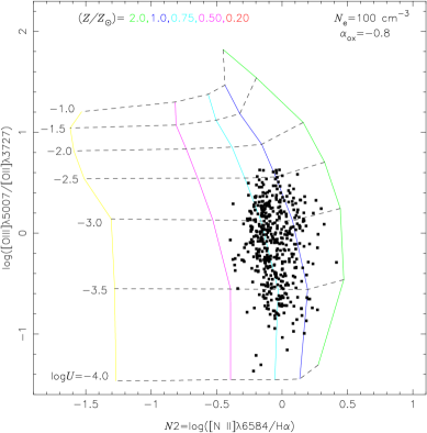
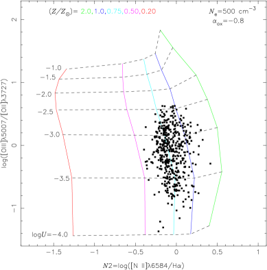
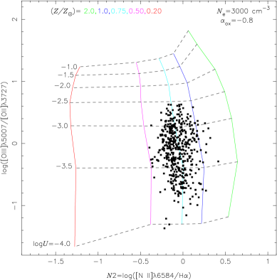
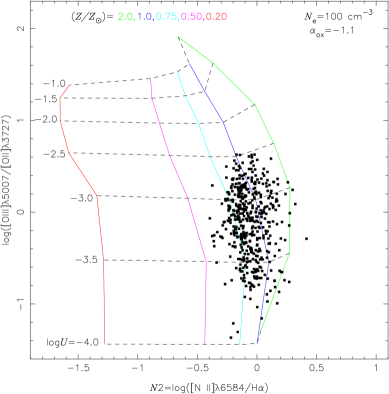
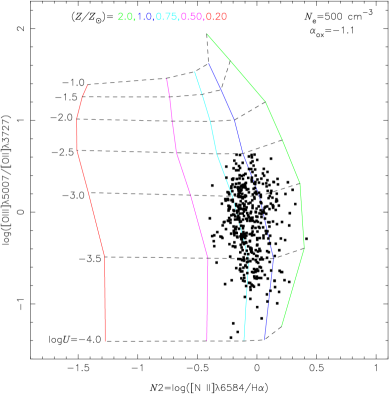
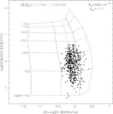
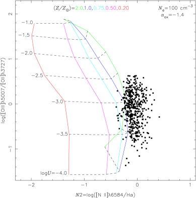
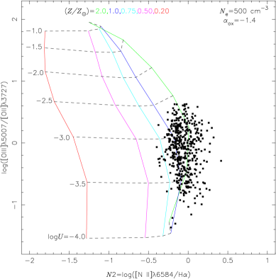
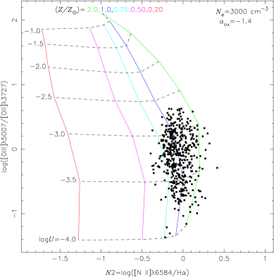
Figure 2: log([O iii]$\lambda 5007$/[O ii]$\lambda 3727$) versus $N2$=log([N ii]$\lambda 6584$/H$\alpha$). Solid lines connect photoionization model results (see Sect. 2.2) with the same metallicity, while dashed lines connect models with same logarithm of the ionization parameter $U$, as indicated. Points represent observational emission-line intensity ratios taken from the SDSS-DR7 (see Sect. 2.1). In each plot, a grid of models assuming different electron density ($N_{\rm e}$) and $\alpha_{ox}$ values, as indicated, are shown.

In Fig. 2, log([O iii]$\lambda$5007/[O ii]$\lambda$3727) versus $N2$=log([N ii]$\lambda$6584/H$\alpha$) diagrams containing the observational data and the photoionization model results previously described are shown. Grids of models assuming distinct suppositions about $N_{\rm e}$ and $\alpha_{ox}$ values are considered in each panel of Fig. 2. It is plausible to note that photoionization models with $N_{\rm e}$= 100, 500, 3000 $\rm cm^{-3}$ and $\alpha_{ox}=-0.8,-1.1$ well reproduce the observational data. As pointed out by Groves et al. (2004) and Feltre, Charlot & Gutkin (2016), we found that optical emission-line ratios are little sensitive to $N_{\rm e}$, under the collisional de-excitation density limit ($N_{\rm e}\><10^{4}\>\rm cm^{-3}$). However, when $\alpha_{ox}=-1.4$ is assumed, the models, in general, under-predict the [N ii]/H$\alpha$. Detailed photoionization modelling carried out by Dors et al. (2017) and bayesian-like comparison between Seyfert 2 optical emission lines and photoionization models by Pérez-Montero et al. (2019) also indicated that $\alpha_{ox}\><\>-1.4$ are representative of the SED of Seyfert 2 AGNs. Therefore, models with $\alpha_{ox}=-1.4$ are not considered in the derivation of the $Z$-$N2$ calibration.

To calibrate the metallicity as a function of the $N2$ index, we calculated the logarithm of the ionization parameter and the metallicity for each object of our sample by linear interpolations between the models shown in Fig. 2. The typical error in emission-line ratio intensities is about 0.1 dex (e.g. Denicoló et al. 2002; Kennicutt et al. 2003). Assuming this uncertainty in the data considered in Fig. 2, we obtained an uncertainty in the $Z$ and $\log U$ interpolated estimations in order of 30% and 0.05 dex, respectively. In the panels of Fig. 3, the relation between $Z/Z_{\odot}$ and $N2$, considering models with distinct $N_{\rm e}$ and $\alpha_{ox}$ values and ranges of $\log U$ are shown. We use the following expression:

$$(Z/Z_{\odot})=a^{N2}+b$$ (2)

to fit the results obtained for the objects in our sample plotted in Fig. 3. The fitting coefficients are listed in Table 1. As it can be seen, the correlation of the derived parameters with $\log U$ is marginal, indicating a very low dependence of the $Z-N2$ relation on the ionization degree in the AGN. On the other hand, a larger dependence of the $Z$-$N2$ relation on $N_{\rm e}$ is found, in the sense that higher (up to a factor of 2) $Z$ estimations are obtained when photoionization models with lower $N_{\rm e}$ are considered, mainly for the high metallicity regime $[(Z/Z_{\odot})\>\ga\>1.0]$. Similarly, a dependence of $Z$-$N2$ on $\alpha_{ox}$ is also derived, in the sense that higher metallicity (up to a factor of 2) is derived if $\alpha_{ox}=-1.1$ is assumed in comparison with those considering $\alpha_{ox}=-0.8$, being the difference between the estimations also more prominent for $(Z/Z_{\odot})\>\ga\>1.0$. Interestingly, an opposite behaviour was found by Dors et al. (2019) for the relation between $Z$ and ultraviolet emission-line ratios (see also Nagao et al. 2006a). We also fitted Eq. 2 considering all points (not discriminating nebular parameters) and the resulting coefficients are listed in Table 1.

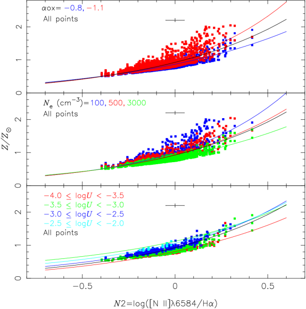
Figure 3: Metallicity ($Z/Z_{\odot}$) versus the $N2$=log([N ii]$\lambda$6584/H$\alpha$). Points represent estimations obtained through linear interpolation between photoionization model results and the observational data presented in Fig. 2. Curves represent the fitting of the equation $(Z/Z_{\odot})=a^{N2}+b$ to the points taking into account different model parameters (indicated in each panel), whose the coefficient fittings are listed in Table 1. Error bars in each panel represents the typical error (0.1 dex) in observational measurements of the $N2$ index (e.g. Denicoló et al. 2002) and the 30% uncertainty in the interpolated values.

Table 1: Values of the $a$ and $b$ coefficients resulting from fittings of the Eq. 2 to the estimations, shown in Fig. 3, for different model parameters. The last line lists the coefficients obtained not discriminating the model parameters.

Model parameter	$a$	$b$
$\log U$
($-$4.0, $-$3.5)	$3.23\pm 0.11$	$-0.19\pm 0.01$
($-$3.5, $-$3.0)	$3.42\pm 0.06$	$-0.12\pm 0.01$
($-$3.0, $-$2.5)	$4.15\pm 0.12$	$-0.01\pm 0.01$
($-$2.5, $-$2.0)	$3.82\pm 1.01$	$+0.06\pm 0.02$
$N_{\rm e}$($\rm cm^{-3}$)
100	$5.58\pm 0.23$	$+0.00\pm 0.01$
500	$4.24\pm 0.12$	$-0.06\pm 0.01$
3000	$2.99\pm 0.04$	$-0.15\pm 0.01$
$\alpha_{ox}$
$-0.8$	$3.14\pm 0.05$	$-0.13\pm 0.01$
$-1.1$	$5.45\pm 0.17$	$-0.01\pm 0.01$
All points	$4.01\pm 0.08$	$-0.07\pm 0.01$

The interpolated values from Fig. 2 made it possible to derive a relation between the logarithm of the ionization parameter and [O iii]/[O ii] line ratio, shown in Fig. 4. The linear regression obtained is:

$$\log U=(0.57\pm 0.01\>x^{2})+(1.38\pm 0.01\>x)-(3.14\pm 0.01),$$ (3)

where $x$=log([O iii]$\lambda$5007/[O ii]$\lambda$3727). We did not find any dependence of this equation on $N_{\rm e}$, $\alpha_{ox}$ and $Z$.

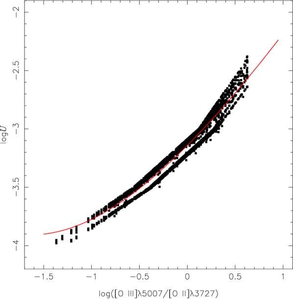
Figure 4: As in Fig. 3 but for the logarithm of the ionization parameter ($\log U$) versus the logarithm of the line ratio [O iii]$\lambda$5007/[O ii]$\lambda$3727. Photoionization model results assuming different parameters are not discriminated. Curve represents the fitting to the points and represented by Eq. 3. The error in the interpolated $\log U$ values is about 0.05 dex.

4 Discussion

Storchi-Bergmann et al. (1994) proposed the use of the $N2$=log([N ii]$\lambda$6584/H$\alpha$) line ratio as an indicator of the ratio between oxygen and hydrogen abundances of H ii regions. These authors obtained a calibration based on O/H abundances calculated through the $T_{\rm e}$-method and observational emission-line intensities of star-forming galaxies. Thereafter, other authors (Raimann et al., 2000; Denicoló et al., 2002; Pettini & Pagel, 2004; Liang et al., 2006; Stasińska, 2006; Nagao et al., 2006b; Yin et al., 2007; Pérez-Montero & Contini, 2009; Marino et al., 2013; Morales-Luis et al., 2014) improved this calibration by including more abundance estimations, mainly for both low and high metallicity ends. The advantage of the $N2$ index over the commonly used metallicity indicator $R_{23}$ is that: ($i$) it does not include the [O ii]$\lambda$3727 line, which makes this line ratio not sensitive to reddening correction and, consequently, useful to dusty object studies (e.g. Xiao et al. 2012); ($ii$) due to the fact that $N2$ involves emission-lines with very close wavelength, it is not affected by uncertainties of flux calibration (Marino et al., 2013), ($iii$) it is accessible in the near infrared at moderate-to-high redshifts (e.g. Cresci et al. 2012; Queyrel et al. 2012), ($iv$) it has a less critical dependence on the ionization parameter, ($v$) it is single-valued with $Z$, and ($vi$) it has a tighter correlation with O/H (Denicoló et al., 2002).

Despite the several advantages, such as other $Z$ indicators, $N2$ index suffers some limitations. Firstly, for any theoretical calibration involving nitrogen lines it is necessary to know the dependence between N/O and O/H abundance ratios (see Pérez-Montero & Contini 2009). For AGNs, this relation was first derived by Dors et al. (2017), who used detailed photoionization model of relatively small (44 objects) sample of local ($z\><\>0.1$) Seyfert 2 AGNs (see also Pérez-Montero et al. 2019). Obviously, it is necessary to obtain N and O abundance estimations for a larger sample of objects at a wider redshift range. Moreover, the dependence between the nitrogen lines and $Z$ (or O/H) is due to the N secondary stellar nucleosynthesis origin [${\rm(N/O)}\approx Z^{2}$] in the “high” metallicity regime [$(Z/Z_{\odot})\>\ga\>0.3$] (e.g. Vila-Costas & Edmunds 1993). Therefore, calibrations involving nitrogen lines are not valid for the low metallicity regime. Finally, the $N2$ index saturates in the very high-metallicity regime (Marino et al., 2013), as it is reported in Sect. 3. In the case of our $Z$-$N2$ calibration, it is valid for the range of $0.3\>\la\>(Z/Z_{\odot})\>\la\>2.0$, which corresponds to $-0.7\>\la\>(N2)\>\la\>0.6$.

Regarding the $Z$-$N2$ calibration dependence on the electron density ($N_{\rm e}$), we found that it is more prominent in the high metallicity regime [$(Z/Z_{\odot})\>\ga 1.0$]. Although $N_{\rm e}$ is easily estimated in AGNs through the dependence of this parameter with the [S ii]$\lambda$6716$\lambda$/6731 line ratio, the observational measurement error of $N2$ ($\sim 0.1$ dex , Denicoló et al. 2002) translates in a $Z$ uncertainty of the order of the one obtained not taking into account the $N_{\rm e}$ effects on our calibration. It can be seen in Fig. 3, where the typical error of $N2$ is shown in the panels. The same result is derived for the effect of $\alpha_{ox}$ on the metallicity estimations, which the $Z$ uncertainty of not knowing $\alpha_{ox}$ is of the order of the uncertainty produced by the observational $N2$ error. It is worth to mention that similar results were derived by Dors et al. (2019). These authors showed that the uncertainties in $Z$ estimations assuming photoionization models with different $N_{\rm e}$ and $\alpha_{ox}$ values are similar to those produced by observational errors of ultraviolet emission-line ratios (see Fig. 5 of their work).

Recently, in Paper I, we compared the AGN Seyfert 2 metallicities (traced by the O/H abundance ratio) and the mass-metallicity relation derived by using most of the available methods in the literature and this analysis will not be repeated here. For simplicity and with the goal to validate our $Z$-$N2$ calibration, we only compare estimations for our sample by using Eq. 2 with those derived by using two calibrations involving nitrogen emission lines, i.e. the first calibration of Storchi-Bergmann et al. (1998) and the Castro et al. (2017) calibration as well as results from bayesian-like approximation proposed by Pérez-Montero et al. (2019).

The $N2$ index combined with [O iii]/H$\beta$ and [O iii]/[O ii] line ratios was proposed as O/H abundance indicator of the NLR of AGNs by Storchi-Bergmann et al. (1998). These authors proposed two theoretical calibrations based on a grid of photoionization models assuming the (N/O)-(O/H) relation derived for nuclear starbursts by Storchi-Bergmann et al. (1994) and given by the relation

$$\rm\log(N/O)=[0.96\>\times\>(12+\log(O/H)]-9.29.$$ (4)

In Paper I, we found that both calibrations of Storchi-Bergmann et al. (1998) produce very similar results (with an average difference of $-0.08$ dex). Therefore, we will consider only the first calibration of these authors given by

$$\begin{array}[]{l@{}l@{}l}\rm(O/H)_{SB98,1}&=&8.34+(0.212\,x)-(0.012\,x^{2})-(0.002\,y)\\ &+&(0.007\,xy)-(0.002\,x^{2}y)+(6.52\times 10^{-4}\,y^{2})\\ &+&(2.27\times 10^{-4}\,xy^{2})+(8.87\times 10^{-5}\,x^{2}y^{2}),\\ \end{array}$$ (8)

where $x$ = [N ii]$\lambda$$\lambda$6548,6584/H$\alpha$ and $y$ = [O iii]$\lambda$$\lambda$4959,5007/H$\beta$. The term O/H above corresponds to 12+log(O/H) and it is converted into metallicity by

$$(Z/Z_{\odot})=10^{8.69-\rm(O/H)_{SB98,1}},$$ (9)

being 8.69 dex the solar oxygen abundance (Asplund et al., 2009; Alende Prieto et al., 2001). The calibration above is valid for $\rm 8.4\>\lid\>12+log(O/H)\>\lid\>9.4$. A correction in the O/H derivation due to the electron density effects on the calibration above is given by

$${\rm(O/H)_{final}=[(O/H)}-0.1\>\times\>\log(N_{\rm e}/300({\rm cm^{-1}}))].$$ (10)

Another calibration for AGNs involving [N ii] lines was proposed by Castro et al. (2017) considering $N2O2$ index. These authors assumed in the photoionization models the following (N/O)-(O/H) relation derived for star-forming regions by Dopita et al. (2000):

$$\begin{array}[]{lll}\log({\rm N/H})&=&-4.57+\log(Z/Z_{\odot});\>{\rm for}\>\log(Z/Z_{\odot})\lid-0.63,\\ \log({\rm N/H})&=&-3.94+2\>\log(Z/Z_{\odot});\>{\rm otherwise}.\\ \end{array}$$ (13)

The calibration derived by Castro et al. (2017) is

$$\begin{array}[]{lll}(Z/Z_{\odot})\!\!\!&=&\!\!\!1.08(\pm 0.19)\times N2O2^{2}+1.78(\pm 0.07)\times N2O2\\ &&+1.24(\pm 0.01).\\ \end{array}$$ (16)

The bayesian-like H ii-Chi-mistry code (hereafter HCm, Pérez-Montero 2014) was used to estimate the O/H and N/O abundance ratios of each object of the sample described in Sect. 2.1. The HCm code is based on a bayesian-like comparison between certain observed emission-line ratios sensitive to total oxygen abundance, nitrogen-to-oxygen ratio, and ionization parameter with the predictions from a large grid of photoionization models. The HCm code does not consider a fixed (N/O)-(O/H) relation. In Pérez-Montero et al. (2019) this code was adapted for AGNs.

In Fig. 5, the differences between the estimations via our $N2$ calibration (Eq. 2) and those via the calibrations proposed by Storchi-Bergmann et al. (1998) and Castro et al. (2017) as well as those derived using the HCm code are plotted against the estimations via Eq. 2. The estimations via our calibration (Eq. 2) were obtained assuming the fitting for all model results, i.e. all $Z-N2$ values, whose coefficients are listed in Table 1. It can be seen in Fig. 5 that a systematic difference is found between the estimations based on our $N2$ calibration and those via Storchi-Bergmann et al. (1998) calibration, in the sense that the latter calibration produces lower and higher $Z$ values for the low and high metallicity regime, respectively. Although similar results have been derived for the difference between the estimations by using the $N2O2$ calibration and those via HCm code, these are less prominent than the one obtained by using Storchi-Bergmann et al. (1998) calibration.

The differences in the $Z$ estimations found in Fig. 5 are probably due to the use of distinct (N/O)-(O/H) relation in the photoionization models used to obtain the calibrations. In order to verify that, in Fig. 6, the (N/O)-(O/H) relations used in the photoionization models to obtain the calibrations considered in Fig. 5 are shown. It can be seen that the (N/O)-(O/H) relation assumed by us in this paper (Eq. 1) and by Castro et al. (2017) (Eq. 13) are very similar to each other, clarifying the lowest $Z$ difference found in Fig. 5. On the other hand, the relation used by Storchi-Bergmann et al. (1998) (Eq. 4) produces lower N/O abundances in comparison with those from the relations assumed in the $N2$ and $N2O2$ calibrations.

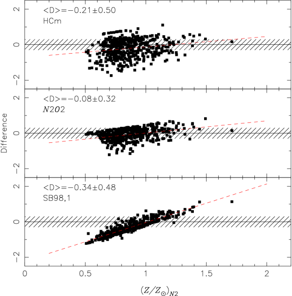
Figure 5: Bottom panel: Difference between the metallicity estimations for our sample of objects (see Sect. 2.1) obtained from our $Z$-$N2$ calibration (Eq. 2) and those from Storchi-Bergmann et al. (1998) calibration versus the $Z$-$N2$ estimations. Middle panel: As the bottom panel but for $Z$-$N2O2$ calibration (Eq. 16) proposed by Castro et al. (2017). Upper panel: As the bottom panel but for estimations obtained by using the HCm code (Pérez-Montero et al., 2019). In each panel, the average and standart desviation of the difference between the estimations are shown. The dashed area indicates the uncertainty of $\pm 0.1$ dex assumed in $Z$ estimations via strong emission-line methods (Denicoló et al., 2002).

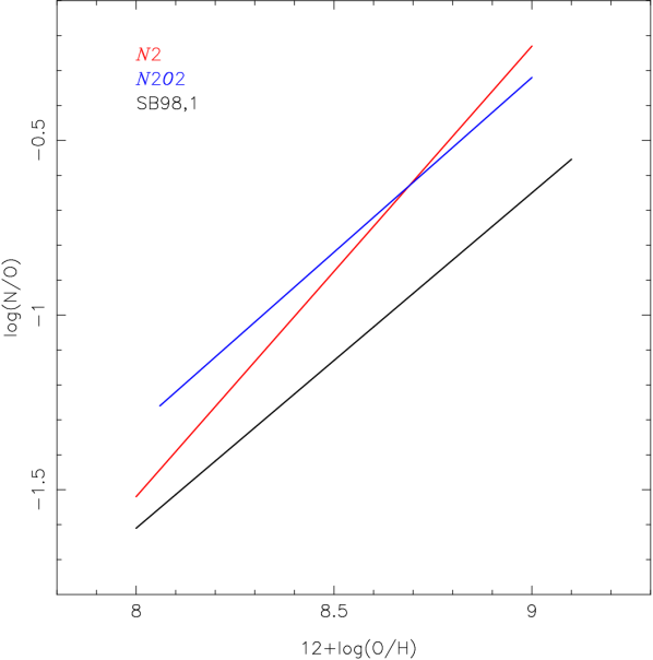
Figure 6: Comparison between the (N/O)-(O/H) relations (represented by the lines) assumed in the photoionization models in this paper (Eq. 1), by Storchi-Bergmann et al. (1998) (Eq. 4), and by Castro et al. (2017) (Eq. 13) to obtain the calibrations represented by the Eqs. 2, 8 and 16, respectively.

Regarding the ionization parameter, few authors have proposed a calibration between $U$ and narrow optical line-ratios of AGNs. For instance, Penston et al. (1990) proposed a calibration between $U$ and the [O ii]$\lambda$3727/[O iii]$\lambda$5007 line ratio. These authors used sequences of photoionization models, taken from Robinson et al. (1987), employing a variety of possible SEDs for the ionizing source and assuming only one value of electron density ($N_{\rm e}=100\>\rm cm^{-3}$) and solar metallicity. The relation derived by Penston et al. (1990) is

$$\log U=-2.74-y,$$ (17)

where $y$=log([O ii]$\lambda$3727/[O ii]$\lambda$5007. Hence the $U$ definition assumed in Robinson et al. (1987) is equal to the one of our models, it is possible to compare estimations derived from their calibration with the ones obtained from our calibration. In Fig. 7, the logarithm of the ionization parameter ($\log U$) calculated by using the Eq. 17 for our sample of objects are compared to those via our calibration (Eq. 3). It can be seen that, in general, the Penston et al. (1990) calibration produces somewhat higher $\log U$ values than those derived from our calibration. This discrepancy, probably, is due to the calibration proposed by Penston et al. (1990) was obtained by using photoionization models with fixed values of $N_{\rm e}$ and $Z$, while in our calibration a semi-empirical aproximation is considered, taken into account a large range of nebular parameter.

Figure 7: Logarithm of the ionization parameter ($\log U$) for our sample (see Sect. 2.1) derived by using the Eq. 17 proposed by Penston et al. (1990) versus those calculated from our calibration (Eq. 3). The line represents the equality between the estimations.

5 Summary and conclusions

We combined results of photoionization model built with the Cloudy code with observational data of 463 confirmed Seyfert 2 nuclei (redshift $z\>\la 0.4$), taken from the Sloan Digital Sky Survey DR7 dataset, in order to obtain a semi-empirical calibration between the metallicity ($Z$) of the Narrow Line Region of these objects and the $N2$=log([N ii]$\lambda$6584/H$\alpha$) emission-line intensity ratio. Our $Z$-$N2$ relation is valid for the range of $0.3\>\la\>(Z/Z_{\odot})\>\la\>2.0$, which corresponds to $-0.7\>\la\>(N2)\>\la\>0.6$. The effects of varying the ionization parameter ($U$), electron density and the slope of the Spectral Energy Distribution on the $Z$ estimations are of the order of the uncertainty produced by the error measurements of $N2$. This result indicates the large reliability of our $Z-N2$ calibration. We also derived a calibration between $\log U$ and the line ratio [O iii]$\lambda$5007/[O ii]$\lambda$3727, less dependent on other nebular parameter.

References

- Abazajian et al. (2009) Abazajian K. N., Adelman-McCarthy J. K., Agüeros M. A. et al., 2009, ApJS, 182, 543
- Alende Prieto et al. (2001) Alende Prieto C., Lambert D. L., Asplund M., 2001, ApJ, 556, L63
- Asplund et al. (2009) Asplund M., Grevesse N., Sauval A. J., Scott P., 2009, ARA&A, 47, 481
- Baldwin et al. (1981) Baldwin J. A., Phillips M. M., Terlevich R., 1981, PASP, 93, 5
- Castellanos et al. (2002) Castellanos M., Díaz A. I., Terlevich E., 2002, MNRAS, 337, 540
- Castro et al. (2017) Castro C. S., Dors O. L., Cardaci M. V., Hägele G. F., MNRAS, 467, 1507
- Contini (2017) Contini M., 2017, MNRAS, 469, 3125
- Contini & Aldrovandi (1983) Contini M., & Aldrovandi S. M. V., 1983, A&A, 127, 15
- Cresci et al. (2012) Cresci G., Mannucci F., Sommariva V., et al. 2012, MNRAS, 421, 262
- Denicoló et al. (2002) Denicoló G., Terlevich R., Terlevich E., 2002, MNRAS, 330, 69
- Dwek & Arendt (1992) Dwek E., Arendt R. G., 1992, ARA&A, 30, 11
- Dopita et al. (2000) Dopita M. A., Kewley L. J., Heisler C. A., Sutherland R. S., 2000, ApJ, 542, 224
- Dors et al. (2012) Dors O. L., Riffel R. A., Cardaci M. V. et al., 2012, 422, 252
- Dors et al. (2014) Dors O. L., Cardaci M. V., Hägele G. F., Krabbe Â. C., 2014, MNRAS, 443, 1291
- Dors et al. (2015) Dors O. L., Cardaci M. V., Hägele G. F., Rodrigues I., Grebel E. K., Pilyugin, L. S., Freitas-Lemes, P., Krabbe Â. C., 2015, MNRAS, 453, 4102
- Dors et al. (2017) Dors O. L., Arellano-Córdoba K. Z., Cardaci M. V., Hägele G. F., 2017, 468, L113
- Dors et al. (2018) Dors O. L., Agarwal B., Hägele G. F., Cardaci M. V., Rydberg C., Riffel R. A., Oliveira A. S., Krabbe A. C., 2018, MNRAS, 479, 2294
- Dors et al. (2019) Dors O. L., Monteiro A. F., Cardaci M. V., Hägele G. F., Krabbe Â. C., 2019, MNRAS, 489, 241
- Dors et al. (2020) Dors O. L., Freitas-Lemes P, Âmores E. B. et al., 2020, MNRAS, 492, 468, Paper I
- Dors & Copetti (2006) Dors O. L., & Copetti M. V. F, 2006, A&A, A&A 452, 473
- Kennicutt et al. (2003) Kennicutt R. C., Bresolin F., Garnett D. R., 2003, ApJ, 591, 801
- Kingdon, Ferland & Feibelman (1995) Kingdon J., Ferland G. J., Feibelman W. A., 1995, ApJ, 439, 793
- Hägele et al. (2008) Hägele, G. F., Dáz, A. I., Terlevich, E., Terlevich, R., Pérez-Montero, E., Cardaci, M. V. 2008, MNRAS, 383, 209
- Ho (1999) Ho L. C., 1999, ApJ, 516, 672
- Izotov et al. (2006) Izotov Y. I., Stasińska G., Meynet G., Guseva N. G., Thuan T. X., 2006, A&A, 448, 955
- Feltre, Charlot & Gutkin (2016) Feltre A., Charlot S., Gutkin J., 2016, MNRAS, 456, 3354
- Ferland et al. (2017) Ferland G. J. et al., 2017, Rev. Mex. Astron. Astrofis., 53, 385
- Garcia-Rojas (2020) García-Rojas J., 2020, arXiv:2001.03388
- Groves et al. (2004) Groves B. A., Dopita M. A., Sutherland R., 2004, ApJ, 153, 75
- Groves et al. (2006) Groves B. A., Heckman T. M., Kauffmann G., 2006, MNRAS, 371, 1559
- Gusev et al. (2012) Gusev A. S., Pilyugin L. S., Sakhibov F., Dodonov S. N., Ezhkova O. V., Khramtsova M. S., 2012, MNRAS, 424, 1930
- do Nascimento et al. (2019) do Nascimento J. C., Storchi-Bergmann T., Mallmann N. D. et al., 2019, 486, 5075
- Kennicutt et al. (2003) Kennicutt R. C., Bresolin F., Garnett D. R., 2003, ApJ, 591, 801
- Kewley et al. (2019) Kewley L. J., Nicholls D. C., Sutherland R. S., 2019, arXiv e-prints, arXiv: 191009730
- Köppen & Hensler (2005) Köppen J., & Hensler G., A&A 434, 531
- Law et al. (2015) Law D. R., Yan R., Bershady M. A. et al., 2015, AJ, 150, 19
- Liang et al. (2006) Liang Y. C., Yin S. Y., Hammer F. et al., 2006, ApJ, 652, 257
- Maiolino & Mannucci (2019) Maiolino, R., & Mannucci, F. 2019, A&ARv, 27, 3
- Marino et al. (2013) Marino R. A., Rosales-Ortega F. F., Sánchez S. F. et al., 2013, A&A, 559, 114
- Matsuoka et al. (2018) Matsuoka, K., Nagao T., Marconi A., Maiolino R., Mannucci F., Cresci G., Terao K., Ikeda H., 2018, A&A, 616L, 4
- Matsuoka et al. (2009) Matsuoka K., Nagao T., Maiolino R., Marconi A., TaniguchiY., 2009, A&A, 503, 721
- Mignoli et al. (2019) Mignoli M., Feltre A., Bongiorno A. et al., 2019, A&A, 626, 9
- Miller et al. (2011) Miller B. P., Brandt W. N., Schneider D. P., Gibson R. R., Steffen A. T., Wu J., 2011, ApJ, 726, 20
- Mólla & Díaz (2005) Mollá M., & Díaz A. I., 2005, MNRAS, 358, 521
- Morales-Luis et al. (2014) Morales-Luis A. B, Pérez-Monterp E., Sánchez Almeida J., Muños-Tuñon C., 2014, ApJ, 797, 81
- Nagao et al. (2006a) Nagao, T., Maiolino, R., Marconi, A. 2006a, A&A, 447, 863
- Nagao et al. (2006b) Nagao, T., Maiolino, R., Marconi, A. 2006b, A&A, 459, 85
- Pagel et al. (1979) Pagel B. E. J., Edmunds M. G., Blackwell D. E., Chun M. S., Smith G., 1979, MNRAS, 189, 95
- Peimbert & Peimbert (2010) Peimbert A., & Peimbert M., 2010, ApJ, 724, 791
- Peimbert, Peimbert, & Delgado-Inglada (2017) Peimbert, M., Peimbert A., Delgado-Inglada G., 2017, PASP, 129, 082001
- Pérez-Montero & Contini (2009) Pérez-Montero E., & Contini T., 2009, MNRAS, 398, 949
- Pérez-Montero (2014) Pérez-Montero E., 2014, MNRAS, 441, 2663
- Pérez-Montero (2017) Pérez-Montero E., PASP, 129, 043001
- Pérez-Montero et al. (2019) Pérez-Montero E., Dors O. L., Vílchez J. M., Garcí-Benito R. et al., 2019, 489, 2652
- Penston et al. (1990) Penston M. V., Robinson A., Alloin D. et al., 1990, A&A, 236, 53
- Pettini & Pagel (2004) Pettini M., & Pagel B. E. J. 2004, MNRAS, 348, L59
- Pilyugin (2003) Pilyugin L. S., 2003, A&A, 399, 1003
- Pilyugin et al. (2004) Pilyugin L. S., Vílchez J. M., Contini T., 2004, A&A, 425, 849
- Pilyugin & Grebel (2016) Pilyugin L. S., & Grebel E. K., 2016, MNRAS, 457, 3678
- Pilyugin & Mattsson (2011) Pilyugin L. S., & Mattsson L., 2011, MNRAS, 412, 1145
- Pilyugin et al. (2012) Pilyugin L. S., Grebel E. K., Mattsson L., 2012, MNRAS, 424, 2316
- Queyrel et al. (2012) Queyrel J., Contini T., Kissler-Patig M., et al. 2012, A&A, 539, A93
- Riffel et al. (2018) Riffel R. A., Hekatelyne C., Freitas I. C., 2018, PASA, 35, 40.
- Riffel et al. (2017) Riffel R. A., Storchi-Bergmann T., Riffel R. et al. 2017, MNRAS, 470, 992
- Raimann et al. (2000) Raimann D., Storchi-Bergmann T., Bica E., Melnick J., Schmitt H. 2000, MNRAS, 316, 559
- Sanders et al. (2016) Sanders R. L., Shapley A. E., Kriek M. et al., 2016, ApJ, 825, L23
- Sanders et al. (2019) Sanders R. L. Shapley, A. E., Reddy N. A. et al., 2019, arXiv e-prints, arXiv:1907.00013
- Robinson et al. (1987) Robinson A., Binette L., Fosbury R. A.E., Tadhunter C. N., 1987, MNRAS, 227, 97
- Rembold et al. (2017) Rembold S. B., Shimoia J., Storchi-Bergmann T. el al., 2017, MNRAS, 472, 4382
- Stasińska (2006) Stasińska G., 2006, A&A, 454, 127L
- Smith (1975) Smith H. E., 1975, ApJ, 199, 591