An interpretable neural network model through piecewise linear approximation

Abstract

Most existing interpretable methods explain a black-box model in a post-hoc manner, which uses simpler models or data analysis techniques to interpret the predictions after the model is learned. However, they (a) may derive contradictory explanations on the same predictions given different methods and data samples, and (b) focus on using simpler models to provide higher descriptive accuracy at the sacrifice of prediction accuracy. To address these issues, we propose a hybrid interpretable model that combines a piecewise linear component and a nonlinear component. The first component describes the explicit feature contributions by piecewise linear approximation to increase the expressiveness of the model. The other component uses a multi-layer perceptron to capture feature interactions and implicit nonlinearity, and increase the prediction performance. Different from the post-hoc approaches, the interpretability is obtained once the model is learned in the form of feature shapes. We also provide a variant to explore higher-order interactions among features to demonstrate that the proposed model is flexible for adaptation. Experiments demonstrate that the proposed model can achieve good interpretability by describing feature shapes while maintaining state-of-the-art accuracy.

1 Introduction

Recent research on interpretability explained the predictions in a post-hoc manner: given a trained predictive model with predicted scores $F\left(\mathbf{x}\right)$, use extracted information to explain how the model made predictions. Such extracted information can be analyzed and displayed by data analysis techniques, such as gradient-based methods Tsang et al. (2018a); Sundararajan et al. (2017); Shrikumar et al. (2017); Yosinski et al. (2015), and sensitivity analysis Ribeiro et al. (2016); Lundberg and Lee (2017), or by using a mimic model $\hat{F}$ to minimize $\|\hat{F}\left(\mathbf{x}\right)-F\left(\mathbf{x}\right)\|$, such as tree- and rule-based models Li et al. (2019); Che et al. (2016); Letham et al. (2015); Wang and Lin (2019). Summing up, the post-hoc methods do not change or improve the underlying predictive model and use simpler forms, such as linear models, to explain the relationships in a complex predictive model, thereby making it easier for users to understand the interpretations.

Post-hoc methods, though effective in interpreting models in an easy-to-understand way, have two limitations: (a) When we use different post-hoc methods to explain the same predictions, the explanations may be contradictory with each other Alvarez-Melis and Jaakkola (2018). The human cost for determining these methods and the samples to train the post-hoc models are prohibitive with larger datasets. Moreover, it is unclear whether we can aggregate different post-hoc explanations Tan et al. (2018); (b) The post-hoc methods focus on using simpler models to provide a higher descriptive accuracy, which measures the degree to which a post-hoc method properly describes the patterns learned by a predictive model. Usually, the simplicity of post-hoc methods helps users understand the patterns, but provides imperfect representations of nonlinear relationships among variables in complex black-box models. Their interpretability is obtained at the expense of prediction accuracy Murdoch et al. (2019).

To overcome these limitations, there is a need for model-based interpretations, which come from the construction of the prediction model Murdoch et al. (2019). Such models (a) have a predefined structure and can readily describe relationships between input features and predictions once the models are learned. It does not require the determination of the post-hoc models and is estimated on all training data, therefore it avoids the interpretations being changed dramatically when different methods or subsets of the data are used. (b) Such models should interpret the relationships between input features and predictions in a simple and explicit way, such as describing feature contributions via providing feature shapes that can be easily understood by users. In the meanwhile, it should be expressive enough to properly fit the data and achieve good prediction performance.

In this work, we propose a hybrid Piecewise Linear and Deep (PiLiD) model under a Wide $\&$ Deep (short for W$\&$D) scheme Cheng et al. (2016) as shown in Figure 1. The proposed model is comprised of a piecewise linear component and a nonlinear component. The first component uses piecewise linear functions to approximate the complex relationships between the input features and predictions. Such a form is explicit enough to describe the feature contributions by providing feature shapes, yet increases the expressiveness of the model. The other component uses a multi-layer perceptron (MLP) to capture the feature interactions and increase the prediction performance. The two components are jointly trained and the interpretability (in the form of piecewise linear functions) is obtained once the model is learned. This work has the following contributions:

• We propose the PiLiD model that enhances the interpretability under a W$\&$D scheme. Different from the post-hoc methods, the interpretability is obtained once the prediction model is learned.

• The proposed PiLiD model is flexible for adaptations. We develop the PiLiB model, a variant to extract interpretable higher-order interactions.

• We integrate a predefined interpretable structure into the linear component to decipher the contribution of features by piecewise linear approximation. Such a form provides explicit feature shapes while preserving high expressiveness.

• As a result of the joint-training scheme, we show that the model can describe complex feature shapes while improving model performance.

2 Related Work

2.1 Wide and Deep Scheme

The Wide $\&$ Deep (W$\&$D) scheme jointly trains a linear model and a deep neural network to benefit from memorization and generalization Cheng et al. (2016). This framework takes advantage of both the Wide (linear model) and Deep (deep neural network) components by jointly training both together, and thus outperforms the models with either Wide or Deep component in a large-scale recommender system Li et al. (2019); Guo et al. (2018); Zheng et al. (2017). The Wide component of the W$\&$D scheme also provides interpretations of the features’ main effect. Hence W$\&$D has been used to develop interpretable models. Tsang et al. Tsang et al. (2018a) developed a model that modified the Deep component to only extract pairwise interactions among features. Similarly, Kraus and Feuerriegel Kraus and Feuerriegel (2019) changed the Deep component to a recurrent neural network to capture the temporal information. Wang and Lin Wang and Lin (2019) proposed a hybrid model, in which an interpretable model and a black-box model function together to obtain a good trade-off between model transparency and performance. Effective as they are, these W$\&$D-based interpretable models’ prediction performance is worse than the complex black-box model (the Deep part alone).

2.2 Interpretable Methods

There are mainly two categories of interpretable machine learning methods. The first refers to post-hoc methods which initially learn an original predictive model and then explain how the model obtains the underlying predictions. This type of models usually fall into two sub-categories, prediction-level and dataset-level interpretations Murdoch et al. (2019).

The prediction-level methods focus on locally explaining why the model makes a particular prediction. They tell users what individual features or feature interactions are the most important by standard data analysis such as the gradient-based methods Tsang et al. (2018a); Sundararajan et al. (2017); Shrikumar et al. (2017); Yosinski et al. (2015), the sensitivity analysis Ribeiro et al. (2016); Lundberg and Lee (2017), the step-wise feature removal approaches Schwab and Karlen (2019), and the mimic models Li et al. (2019); Che et al. (2016); Letham et al. (2015); Wang and Lin (2019). In contrast, the dataset-level methods are interested in global explanations that explore more general relationships learned by the models. Tan et al. Tan et al. (2018) described feature contributions by providing a global additive value function. Both prediction- and dataset-level methods suffer from the aforementioned drawbacks of post-hoc scheme.

Another category of approaches predefines an interpretable structure, and provides insight into relationships between input features and predictions once the model is learned Kraus and Feuerriegel (2019). Generalized additive model (GAM) can model extreme nonlinearity on individual features Hastie and Tibshirani (1986); Lou et al. (2012), but it cannot model feature interactions. In this regard, Lou et al. Lou et al. (2013) developed the GA²M model, which first learns a base GAM without any interactions and then selects a number of pairwise interactions that minimize residuals. Unfortunately, the obtained individual and interacting feature contributions can be extremely complex because there is no regularization on their shapes, and this model is slow to converge. For this reason, Tsang et al. Tsang et al. (2018b) divided a neural network into several same-sized blocks and used $L_{0}$ regularization to model both uni-variate and high-order interactions, however, only a subset of individual features can be interpreted and the accuracy decreases because the model does not capture the nonlinearity other than the learned feature interactions. The main challenge, as the main purpose of this paper, is to come up with a structure that is simple enough to help users understand the rationale behind the predictions, while keeping the model sophisticated to take care of the non-interpretable nonlinearity in the data.

3 The Proposed PiLiD Model

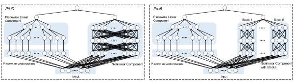
Figure 1: The proposed PiLiD (left) and PiLiB (right) models. In PiLiB, the whole neural network in the nonlinear component of PiLiD is replaced with B same-sized smaller neural networks (blocks).

3.1 Problem Setting

Vectors are represented by boldface lower-case letters, for example x. Note that the index for $i$-th vector is in brackets, such as $\textbf{x}_{(i)}$ is the $i$-th data point, and the $j$-th element of a vector w is $\textbf{w}_{j}$; matrices are denoted by boldface capital letters, for example W and the element $(i,j)$ of W is $W_{i,j}$. Let $\{\textbf{x}_{(i)},y_{i}\}_{i=1}^{N}$ be a set of $N$ data samples, where $\textbf{x}_{(i)}=(x_{i,1},\ldots,x_{i,j},\ldots,x_{i,m})^{T}\in\mathbb{R}^{m}$ is the $i$-th data point described by $m$ features, and $y_{i}$ is a real value (class label) to be predicted in regression (classification) problems.

We assume that there exists a mapping function describing the relationship between the prediction and the individual features (main effects) and interacting features (interaction effects). To predict ${y_{i}}$, we define:

$$U\left({y_{i}}\right)=w_{0}+\sum\limits_{j=1}^{m}{u_{j}\left({{x_{i,j}}}\right)}+u\left({{x_{i,1}},\ldots{x_{i,m}}}\right)$$ (1)

where $w_{0}$ is a constant term, $u_{j}\left(\cdot\right)$ is a marginal value function of $j$-th feature, and $u\left(\cdot\right)$ is a function of all features. Eq.(1) describes (a) a regression model if $U(\cdot)$ is the identity, and (b) a classification model if $U(\cdot)$ is the logistic function of the identity.

Given the following definitions, we use piecewise linear functions to approximate the marginal value functions.

Definition 1.

The characteristic points are some predefined values to partition the whole feature value scale into several pieces.

For categorical features, the characteristic points ${\Psi_{j}}=\{x_{i,j}|i=1,\ldots,N\}$ are all unique feature values. Let $\varphi_{j}^{1},\ldots,\varphi_{j}^{k},\ldots,\varphi_{j}^{{n_{j}}}$ be the ordered values of $\Psi_{j},\varphi_{j}^{k}<\varphi_{j}^{k+1},k=1,\ldots,{n_{j}}-1$, where ${n_{j}}=\left|{{\Psi_{j}}}\right|$ and ${n_{j}}\leq N$. For numerical features, let $\left[\alpha_{j},\beta_{j}\right]$, where $\alpha_{j}=min\{x_{i,j}|i=1,\ldots,N\}$ and $\beta_{j}=max\{x_{i,j}|i=1,\ldots,N\}$, be the whole evaluation value scale. We partition the scale into $\gamma_{j}$ equal sub-intervals $[\varphi^{0}_{j},\varphi^{1}_{j}],[\varphi_{j}^{1},\varphi_{j}^{2}],\dots,[\varphi_{j}^{\gamma_{j}-1},\varphi_{j}^{\gamma_{j}}]$, where $\varphi_{j}^{k}={\alpha_{j}}+\frac{k}{{{\gamma_{j}}}}\left({{\beta_{j}}-{\alpha_{j}}}\right),k=0,1,\ldots{\gamma_{j}}$ are characteristic points.

Definition 2.

The feature vector $\boldsymbol{\Phi}_{(i)}\in\mathbb{R}^{\gamma},\gamma={\sum\nolimits_{j=1}^{m}{{\gamma_{j}}}}$ of data point $\textbf{x}_{(i)}$ is defined as follows:

where $\phi_{i,j}^{k_{j}}=\left\{\begin{array}[]{l}1,\quad x_{i,j}>\varphi_{j}^{{k_{j}}},\\ \frac{{x_{i,j}-\varphi_{j}^{k_{j}-1}}}{{\varphi_{j}^{{k_{j}}}-\varphi_{j}^{k_{j}-1}}},\>\varphi_{j}^{k_{j}-1}\leq x_{i,j}\leq\varphi_{j}^{{k_{j}}},\\ 0,\quad\quad\text{otherwise}.\end{array}\right.j=1,\dots,m,$ and ${k_{j}}=1,\dots,\gamma_{j}.$

Definition 3.

The marginal value vector u is defined as:

$$\textbf{u}={\left({\Delta_{1}^{1},\ldots,\Delta_{1}^{{\gamma_{1}}},\ldots,\Delta_{j}^{{k_{j}}},\ldots,\Delta_{m}^{1},\ldots,\Delta_{m}^{{\gamma_{m}}}}\right)^{T}}$$ (3)

where $\Delta_{j}^{k_{j}}=u_{j}(\varphi_{j}^{k_{j}})-u_{j}(\varphi_{j}^{k_{j}-1}),j=1,\dots,m,$ and $k_{j}=1,\dots,\gamma_{j}$, is the difference of marginal values between two consecutive characteristic points.

We use an MLP to approximate the interaction effects $u\left({{x_{i,1}},\ldots{x_{i,m}}}\right)$. Here it is a feed-forward neural network with $L$ hidden layers. There are $p_{l}$ hidden units in the $l$-the layer and $p_{0}=m$. The layer matrices are denoted by $\textbf{W}^{l}\in\mathbb{R}^{p_{l}\times p_{l-1}}$, and bias vectors are denoted by $\textbf{b}^{l}\in\mathbb{R}^{p_{l}},l=1,\ldots,L$. The non-linear activation function is denoted as $\phi(\cdot)$. Let $\textbf{w}^{y}\in\mathbb{R}^{p_{L}}$ and $b^{y}\in\mathbb{R}$ be the final weight vector and bias for the output $y$. In this way, the MLP with $L$ layers can be represented by:

$$\textbf{h}^{0} =\textbf{x},$$ (4)

$$\textbf{h}^{l} =\phi\left(\textbf{W}^{l}\textbf{h}^{l-1}+\textbf{b}^{l}\right),l=1,\ldots,L,$$ (5)

$$y =\left(\textbf{w}^{y}\right)^{T}\textbf{h}^{L}+b^{y}.$$ (6)

3.2 Model Description and Training Process

Given Definition 3 and Eq.(6), the Eq.(1) can be reformulated as follows:

$$U\left({y_{i}}\right)=w_{0}+\textbf{u}^{T}\boldsymbol{\Phi}_{i}+u\left({{x_{i,1}},\ldots{x_{i,m}}}\right)$$ (7)

According to Definition 2, the vectorized input layer in piecewise linear component transforms the original data into a ‘wider’ vector by piecewise linear partition. The input of each unit in this layer corresponds to an element in vector $\boldsymbol{\Phi}$, and every $\gamma_{j}$ units are decomposed from one feature. The first layer in the piecewise linear component has $\sum\nolimits_{j=1}^{m}{{\gamma_{j}}}$ units and has a form $\textbf{y}=\textbf{w}^{T}\boldsymbol{\Phi}+\textbf{b}$, where $\textbf{w}=\left(w_{1},\ldots,w_{\gamma}\right)^{T}$ and $\textbf{b}=\left(b_{1},\ldots,b_{\gamma}\right)^{T}$. There is no any activation function. The next layer groups every $\gamma_{j}$ units ($m$ groups in total), and then sums the outputs of units in each group. Note that when $\gamma_{j}=1,j=1,\ldots,m$, the piecewise linear component PiLiD degenerates to a simple linear model providing a single value describing feature contributions, i.e., feature attributions. When $\gamma_{j}\rightarrow\infty$, all feature values become characteristic points, PiLiD has to fit the curve point-by-point. Thus, it can fit any curve given sufficient data. Without the constrain in $\gamma_{j}$, it may use an extremely complex shape to fit the curve, causing the over-fitting problem.

The outputs of two components are fed into a specific loss function for joint training. The joint training process uses the mini-batch stochastic optimization algorithm to back-propagate the gradients from both components at the same time. The general loss function is:

$$\mathcal{R}\left({\boldsymbol{\omega},\textbf{w},\textbf{b},\boldsymbol{\theta}}\right) =\frac{1}{N}\left({\sum\limits_{i=1}^{N}{\mathcal{L}\left({h\left({\textbf{x}_{(i)};{\boldsymbol{\omega},\textbf{w},\textbf{b},\boldsymbol{\theta}}}\right),{y_{i}}}\right)}}\right)$$

$$+\lambda\Omega\left({\boldsymbol{\omega},\textbf{w},\textbf{b},\boldsymbol{\theta}}\right)$$ (8)

where $h(\cdot;{\boldsymbol{\omega},\textbf{w},\textbf{b},\boldsymbol{\theta}})$ is a neural network with ${\boldsymbol{\omega},\textbf{w},\textbf{b},\boldsymbol{\theta}}$ parameters, ${\boldsymbol{\omega},\textbf{w},\textbf{b}}$ are the vectors of parameters in the piecewise linear component, ${\boldsymbol{\theta}}$ are the parameters, including weights matrices $\textbf{W}^{l},l=1,\ldots,L$, bias vectors $\textbf{b}^{l},l=1,\ldots,L$, weight vector $\textbf{w}^{y}$ and bias term $b^{y}$ for the output of nonlinear component, $\mathcal{L(\cdot)}$ is the loss function. Specifically, $\mathcal{L(\cdot)}$ is the cross-entropy loss for classification problems and the mean square error for regression problems. $\lambda$ is a predefined coefficient for the regularization function $\Omega(\cdot)$ that can be $L_{1}$ or $L_{2}$ regularization.

The gradient-based algorithms can make the optimal solution robust and fast to converge by initializing the parameters in a neural network LeCun et al. (2015). In this study, the parameters in the piecewise linear component are not randomly initialized because their optimal values are supposed to indicate the contributions of individual features to the predictions. For this reason, we use the parameters obtained by a simple linear regression to initialize the parameters in the piecewise linear component. Such initialization forces the optimization algorithm starts from a more promising and interpretable solution region. As for the nonlinear component, we use a standard Gaussian initialization. The pseudo code for learning the proposed model is presented in Algorithm 1 (for brevity, we raise a regression problem as an example):

Algorithm 1 Training process for the proposed PiLiD.

0:  Training data $\{\textbf{x}_{(i)},y_{i}\}^{N}_{i=1}$, structure of nonlinear component $L$, predefined number of sub-intervals $\gamma_{j},j=1,\dots,m$, type of loss function $\mathcal{L}(\cdot)$, regularization term $\lambda$ and regularization type $\Omega(\cdot)$, initialization coefficient $\sigma$ for nonlinear component, number of epoch and Batch size.

0:  Parameters ${\boldsymbol{\omega}^{*}},{\textbf{w}^{*}},{\textbf{b}^{*}},{\boldsymbol{\theta}^{*}}=\mathop{\arg\min}\limits_{\boldsymbol{\omega},\textbf{w},\textbf{b},\boldsymbol{\theta}}\{\mathcal{R}({\boldsymbol{\omega},\textbf{w},\textbf{b},\boldsymbol{\theta}})\}$.

1:  Vectorize the feature values in $\textbf{x}_{(i)}$ into $\boldsymbol{\Phi}_{(i)}$ according to Definition 2. Let $\boldsymbol{\Phi}=(\boldsymbol{\Phi}_{(1)},\ldots,\boldsymbol{\Phi}_{(N)})^{T}$ and $\textbf{y}=(y_{1},\ldots,y_{N})^{T}$.

2:  Initialize $\boldsymbol{\omega}\leftarrow(1,\ldots,1)^{T}$, $\textbf{w}\leftarrow\left(\boldsymbol{\Phi}\boldsymbol{\Phi}^{T}\right)^{-1}\boldsymbol{\Phi}\textbf{y}$, $\textbf{b}\leftarrow(0,\ldots,0)^{T}$, $\textbf{W}^{l}\leftarrow\mathcal{N}\left(0,\sigma\right)$, and $\textbf{b}^{l}\leftarrow(0,\ldots,0)^{T},l=1,\ldots,L$.

3:  Standard mini-batch stochastic gradient optimization algorithm.

3.3 A Variant

To explore interacting effects in nonlinear component and demonstrate the flexibility of the proposed model, we substitute the nonlinear component with the state-of-the-art Neural Interaction Transparency (NIT) model to decipher the high-order feature interactions Tsang et al. (2018b).

The original NIT model partitions a whole feed-forward neural network into several ‘blocks’ with the same size. It uses the $L_{0}$ regularization to force some hidden units to have zero weights in each ‘block’, and adds an extra term $\mathcal{L_{K}}$ in the loss function to encourage the model to learn smaller-sized interactions. We refer interested readers to Tsang et al.Tsang et al. (2018b). In this work, we propose a variant of PiLiD, namely the Piecewise Linear and Blocks (PiLiB) to model all individual features and important interacting features.

The piecewise linear component in PiLiB is same as that in PiLiD. The nonlinear component is divided into $B$ same-sized block (shown on the right in Figure 1). The loss function of PiLiD is:

$$\mathcal{R}_{PiLiB}=\mathcal{L_{K}}^{\prime}+\frac{1}{N}\times(\sum\limits_{i=1}^{N}{}\mathcal{L}(h(\textbf{x}_{(i)};\boldsymbol{\omega},\textbf{w},\textbf{b},\tilde{\textbf{W}}^{1}\odot$$

$$\quad\quad\quad\quad\quad\mathcal{T}(\textbf{G}(\boldsymbol{\Phi}))),\{\textbf{W}^{l}\}_{l=2}^{L+1},\{\textbf{b}^{l}\}_{l=2}^{L+1},{y_{i}}))$$ (9)

$$\mathcal{L_{K}}^{\prime}=\max\left\{{\left({\mathop{\max}\limits_{i}\hat{k}_{i}}\right)-K,0}\right\}$$

$$\quad\quad\quad\quad\quad+\lambda_{0}{{\sum\limits_{i=1}^{B}{\left({{{\hat{k}}_{i}}-2}\right)}}\mathord{\left/{\vphantom{{\sum\limits_{i=1}^{B}{\left({{{\hat{k}}_{i}}-2}\right)}}{\sum\nolimits_{i=1}^{B}{1\left({k\neq 0}\right)}}}}\right.\kern-1.2pt}{\sum\nolimits_{i=1}^{B}{\mathbbm{1}\left({\hat{k}_{i}\neq 0}\right)}}}$$ (10)

Note that $\textbf{G}\approx 1$ if a feature is active in a block, thus the estimated interaction order is defined as $\hat{k}_{i}=\sum\limits_{j=1}^{m}{G_{ij}(\Phi_{ij})},\forall i=1,\ldots,B$. The first term in $\mathcal{L_{K}}^{\prime}$ limits the maximum interaction order to be equal to or less than $K$. Different with Tsang et al. Tsang et al. (2018b), the second term encourages the model to learn pairwise interactions. In this way, we push the modelling of the main effects to the piecewise linear component and the pairwise interactions to the nonlinear component. The algorithm for training parameters in PiLiB is in supplementary materials.

Table 1: Average $MSE$ for regression problems when $N=20000$ (The best results are marked in bold. The number following PiLiD is the predefined number of intervals for piecewise linear functions.).

# features	10	20	30	40	50
PiLiD-1	0.2677 $\pm$ 0.0073	0.3041 $\pm$ 0.0147	0.2770 $\pm$ 0.0060	0.3406 $\pm$ 0.0139	0.3522 $\pm$ 0.0121
PiLiD-5	0.2666 $\pm$ 0.0070	0.3042 $\pm$ 0.0079	0.2752 $\pm$ 0.0067	0.3318 $\pm$ 0.0155	0.3553 $\pm$ 0.0152
PiLiD-10	0.2678 $\pm$ 0.0089	0.3060 $\pm$ 0.0158	0.2793 $\pm$ 0.0141	0.3383 $\pm$ 0.0184	0.3491 $\pm$ 0.0178
PiLiD-15	0.2662 $\pm$ 0.0070	0.3039 $\pm$ 0.0124	0.2760 $\pm$ 0.0087	0.3291 $\pm$ 0.0133	0.3473 $\pm$ 0.0134
PiLiD-20	0.2657 $\pm$ 0.0058	0.3023 $\pm$ 0.0077	0.2793 $\pm$ 0.0064	0.3296 $\pm$ 0.0129	0.3448 $\pm$ 0.0144
MLP	0.2705 $\pm$ 0.0133	0.3092 $\pm$ 0.0067	0.2816 $\pm$ 0.0035	0.3599 $\pm$ 0.0218	0.3681 $\pm$ 0.0236
SVM (rbf kernel)	0.2801 $\pm$ 0.0047	0.3262 $\pm$ 0.0079	0.2856 $\pm$ 0.0058	0.3935 $\pm$ 0.0083	0.3865 $\pm$ 0.0073
Random Forest	0.2703 $\pm$ 0.0052	0.3131 $\pm$ 0.0121	0.3160 $\pm$ 0.0069	0.4032 $\pm$ 0.0081	0.3998 $\pm$ 0.0083
Linear Regression	0.3518 $\pm$ 0.0053	0.3952 $\pm$ 0.0095	0.2873 $\pm$ 0.0058	0.3925 $\pm$ 0.0082	0.4176 $\pm$ 0.0098
GAM	0.2976 $\pm$ 0.0040	0.3250 $\pm$ 0.0060	0.2804 $\pm$ 0.0050	0.3808 $\pm$ 0.0052	0.3726 $\pm$ 0.0068

Table 2: Averaged $MSE$ given proposed initialization and Gaussian initialization (${}^{*},^{**}$ are significantly different at 10% and 5% levels.).

	$\gamma_{j}=1$		$\gamma_{j}=5$		$\gamma_{j}=10$		$\gamma_{j}=15$		$\gamma_{j}=20$
# objects	Initi.	G. Ini.	Initi.	G. Ini.	Initi.	G. Ini.	Initi.	G. Ini.	Initi.	G. Ini.
5000	0.3755∗∗	0.3860	0.3704	0.3625	0.3752	0.3909	0.3684	0.3603	0.3686	0.3666
10000	0.3427∗∗	0.3612	0.3407	0.3305	0.3348∗∗	0.3443	0.3359∗∗	0.3477	0.3341∗∗	0.3428
15000	0.3182	0.3105	0.3147∗∗	0.3251	0.3101∗	0.3155	0.3105∗	0.3176	0.3087∗∗	0.3275
20000	0.3083∗∗	0.3273	0.3066	0.3091	0.3081∗∗	0.3209	0.3045	0.3091	0.3044	0.3055

4 Experiments

Our experiments are conducted on synthetic and real datasets. The simulations aim to answer the following questions: (a) Can the proposed PiLiD accurately describe the actual marginal value functions while outperforming other predictive models? (b) Does the initialization process help improve interpretability and accuracy? The experiments on real datasets aim to show the advantages of PiLiD and PiLiB over several state-of-the-art interpretable methods.

4.1 Simulations

The synthetic data is generated as follows: (a) Randomly determine the coefficients of $m$ polynomial functions (in 10 degrees) as the actual marginal value functions. (b) Randomly determine $N$ objects and their feature values from interval $[0,1]$. (c) Use actual marginal value functions to calculate the marginal values of $N$ objects and randomly add some feature interactions. (d) For regression problem, $y$ is the summation of $m$ marginal values and selected interactions; For binary classification problem, we use a logistic function to assign 0 and 1 labels. In this section, we present the results of regression problems due to length limit. The classification problem has similar results, which are presented in the supplementary materials.

The MLP used in PiLiD has a 100-200-400-400-200-100-1 structure. We use ADAM with 0.005 learning rate as the standard optimizer in Algorithm 1. For each problem setting, we run 20 trials. 80% is selected as the training set and 20% as the testing set. We present experimental results of regression problems with $N=20000$ in Table 1. The full simulation results can refer to supplementary materials.

When the synthetic data size is small, both MLP and PiLiD perform worse than classic statistical learning models (see results in supplementary materials when $N=5000$), such as SVM and Random Forest. When the data size is larger, more data are fed into the neural network, as a result, both MLP and PiLiD perform better than statistical learning models (Table 1). Encouragingly, we find that PiLiD outperforms MLP in most tasks given the same neural network setting and the number of iterations. At last, as the increase in the number of predefined intervals $\gamma_{j}$, the piecewise linear component becomes more complex, and in turn increases the model accuracy. This indicates that the piecewise linear component could actually improve the performance if the learned interpretability is close to the actual one. Nevertheless, we suggest setting $\gamma_{j}=5,10,15$ to avoid the overfitting problem and additional computational cost.

Table 3: Predictive performance of the proposed PiLiD and PiLiB. In both models, $\gamma_{j}=5$. In NIT and PiLiB, $K=3,B=20$.

	bike sharing (MSE)	bank marketing (AUC)	spambase (AUC)	skill (AUC)
PiLiD	0.068$\pm$0.0087	0.938$\pm$0.0031	0.978$\pm$0.0021	0.877$\pm$0.0058
PiLiB	0.107$\pm$0.0109	0.924$\pm$0.0028	0.965$\pm$0.0047	0.862$\pm$0.0047
MLP	0.071$\pm$0.0091	0.929$\pm$0.0027	0.966$\pm$0.0031	0.864$\pm$0.0049
NIT	0.090$\pm$0.0088	0.894$\pm$0.0367	0.961$\pm$0.0039	0.858$\pm$0.0051
GA	0.137$\pm$0.0023	0.882$\pm$0.0098	0.935$\pm$0.0023	0.851$\pm$0.0037
GAM	0.215$\pm$0.0015	0.856$\pm$0.0032	0.923$\pm$0.0009	0.811$\pm$0.0023
GA2M	0.101$\pm$0.0021	0.902$\pm$0.0055	0.959$\pm$0.0013	0.856$\pm$0.0038

Summing up, the proposed PiLiD performs better because (a) the piecewise linear form increases model expressiveness; and (b) the proposed initialization in Algorithm 1 and the joint training process help obtain optimal solutions (see results in Table 2). To demonstrate that the proposed initialization helps obtain rational interpretations, we provide an example of learned marginal value functions by two initializations in Figure 2. Obviously, although Gaussian initialization can sometimes obtain results as accurate as the proposed initialization, it fails to properly describe the actual marginal value functions.

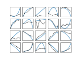
(a) The proposed initialization.

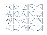
(b) The Gaussian initialization.

Figure 2: An example of the learned marginal value functions given different initializations when $m=20,N=15000,\gamma_{j}=5$. All curves are averaged over 20 trials. The solid blue curves are the actual functions and the dashed black curves are learned functions.

4.2 Real Data

Table 4: Description on datasets.

	Bike share	Bank market	Spambase	Skill
# objects	17,379	40,787	4,601	3,302
# features	15	48	57	18

We conduct experiments using four real datasets to compare the prediction performance of the proposed PiLiD and PiLiB, and a set of baseline models including global additive explanation model (GA) Tan et al. (2018), GAM Lou et al. (2012), GA²M Lou et al. (2013), and NIT Tsang et al. (2018b) models. The datasets are described in Table 4.

Table 3 presents the performance of different models. Comparing with NIT and MLP, the proposed PiLiD performs better because it benefits from the extra piecewise linear component that considers more complex feature shapes and the jointly training process. Comparing with the GAM family, although GAMs can model extremely complex feature shapes, they cannot account for possible higher-order interactions (except for GA²M, which only deals with the pairwise interactions). Therefore, both PiLiD and PiLiB outperform all GAMs.

(a) $\gamma_{j}=1$

(b) $\gamma_{j}=5$

(c) $\gamma_{j}=10$

(d) $\gamma_{j}=15$.

(e) $\gamma_{j}=20$

Figure 3: The visualization of learned feature shapes (Age) in dataset Skill by PiLiD.

To demonstrate the interpretability of PiLiD and PiLiB, we present feature shapes of Age in dataset Skill given different $\gamma_{j}$. First, from Figure 3(a) and other plots, we stress the importance of providing feature shapes rather than only feature attributions that uses a single value to describe the feature contribution. All other plots ($\gamma_{j}\geq 1$) can capture the changing tendency of the relationship between Age and players’ skill estimation (prediction). Such tendency indicates that, at first, the aging process positively affects players’ skill because they can gain experience over time, but it changes when players are older because their response speed is affected. Second, as stated in Schwab and Karlen Schwab and Karlen (2019), the explanations should be robust. From plots (b) to (e) in Figure 3, the obtained feature shapes have a similar tendency given predefined number of intervals. That is because the proposed initialization enforces the optimization to start from a more promising region, and thus makes the interpretability more robust and stable.

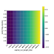
(a) Interaction effects between average length of uninterrupted sequences of capital letters and word frequency of receive.

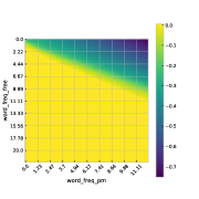
(b) Interaction effects between word frequency of pm and free.

Figure 4: The visualization of interacting features in dataset Spambase by PiLiB.

In Figure 4, we present an example of the learned interacting effects by PiLiB. These relationships help to understand why an email is classified as spam. For example, an email is more likely to be a spam if we observe the overuse of continuous capital letters and less use of the term receive. Interpreting and applying these extracted interactions needs further examinations, and will be our future work.

5 Conclusion

We propose a hybrid interpretable model that uses piecewise linear functions to approximate the individual feature contributions. It is flexible to adapt for other model structures. The experiments demonstrate that the model is explicit enough for users to understand and also has state-of-the-art prediction performance. This research shed new light on the joint learning for interpretability and predictability, and the feasibility of using the learned interpretability to enhance the prediction performance.

6 Supplementary Material

6.1 Algorithm for Training PiLiB

Given loss function $\mathcal{R}_{PiLiB}$, the training process of PiLiB is in two phases. At the first stage, we jointly train the linear component with parameter regularization $\Omega(\cdot)$ and deep component with only $L_{0}$ regularization. After the maximum interaction order in the deep component is smaller or equal to the allowable $K$, we go to next phase. In the second phase, the trained ‘masks’ for the first layer are fixed and on this basis, we optimize all parameters in the model with standard regularization. The training process can be summarized by Algorithm 2.

Algorithm 2 Training process for PiLiB.

0:  Training data $\{\textbf{x}_{(i)},y_{i}\}^{N}_{i=1}$, structure of deep component $L$, predefined number of sub-intervals $\gamma_{j},j=1,\dots,m$, type of loss function $\mathcal{L}(\cdot)$, regularization term $\lambda$, $\lambda_{0}$ and regularization type $\Omega(\cdot)$, maximum interaction order $K$, number of blocks $B$, initialization coefficient $\sigma$ for deep component, number of epoch and Batch size.

0:  Parameters ${\boldsymbol{\omega}^{*}},{\textbf{w}^{*}},{\textbf{b}^{*}},{\boldsymbol{\theta}^{*}},\textbf{G}^{*}$.

1:  Steps 1 and 2 in Algorithm 1 in main paper.

2:  while $\mathop{\max}\limits_{i\in\{1,\ldots,B\}}{\hat{k}_{i}}\geq K$ do

3:     Optimize loss function: $\mathcal{R}_{1}=\mathcal{R}_{PiLiB}+\lambda\Omega\left(\boldsymbol{\omega},{\textbf{w}},{\textbf{b}}\right)$.

4:     ${\boldsymbol{\omega}^{*}},{\textbf{w}^{*}},{\textbf{b}^{*}},\textbf{G}^{*},{\boldsymbol{\theta}^{*}}=\mathop{\arg\min}\limits_{\boldsymbol{\omega},\textbf{w},\textbf{b},\textbf{G},\boldsymbol{\theta}}\{\mathcal{R}_{1}({\boldsymbol{\omega},\textbf{w},\textbf{b},\textbf{G},\boldsymbol{\theta}})\}$.

5:  end while

6:  Fix $\textbf{G}^{*}$, and initialize the parameters $\{{\boldsymbol{\omega}},{\textbf{w}},{\textbf{b}},{\boldsymbol{\theta}}\}\leftarrow\{{\boldsymbol{\omega}^{*}},{\textbf{w}^{*}},{\textbf{b}^{*}},{\boldsymbol{\theta}^{*}}\}$.

7:  Optimize $\mathcal{R}_{2}=\frac{1}{N}\left({\sum\limits_{i=1}^{N}{\mathcal{L}\left({h\left({\textbf{x}_{(i)};{\boldsymbol{\omega},\textbf{w},\textbf{b},{\tilde{\textbf{W}}^{1}\odot\mathcal{T}\left(\textbf{G}^{*}\right)}}}\right),\{\textbf{W}^{l}\}_{l=2}^{L+1},\{\textbf{b}^{l}\}_{l=2}^{L+1},{y_{i}}}\right)}}\right)+\lambda\Omega\left(\boldsymbol{\omega},\textbf{w},\textbf{b},\boldsymbol{\theta}\right)$ by standard mini-batch stochastic gradient.

8:  ${\boldsymbol{\omega}^{*}},{\textbf{w}^{*}},{\textbf{b}^{*}},{\boldsymbol{\theta}^{*}}=\mathop{\arg\min}\limits_{\boldsymbol{\omega},\textbf{w},\textbf{b},\boldsymbol{\theta}}\{\mathcal{R}_{2}({\boldsymbol{\omega},\textbf{w},\textbf{b},\boldsymbol{\theta}})\}$.

6.2 Extend Simulation Results

Here we present full simulation results of regression and classification problems. Tables 5 to 10 present the simulation results given different numbers of objects and features for two problems. We emphasize three interesting patterns:

• As stated in main paper, when the dataset is smaller, for example $N=5000$, since the proposed PiLiD is under a deep learning scheme, it requires sufficient data to train parameters. Therefore, PiLiD and MLP’s performance on simulation data are worse than some traditional predictive models. However, when the datasets are larger ($N=10000,15000,20000$), the PiLiD perform better.

• In classification problems, the performance of the proposed PiLiD is on a par with or comparable to MLP. The proposed PiLiD performs better than MLP given same regression problem settings. That is because the pretriaing process in Algorithm 1 helps PiLiD find better solutions. Moreover, the piecewise linear form also increases the expressiveness of the entire model, thereby being more powerful than a pure MLP.

• There is a tendency that the predictive performance increases along with the increase of predefined number of intervals. It makes sense because the larger number of intervals, the more complex the linear component. As stated in main paper, an extreme simulation is let $\gamma_{j}\rightarrow\infty$, then the linear component becomes a GAM, which is more powerful than linear models. However, larger number of intervals will require more computational cost and data samples, as a trade-off, we suggest using $\gamma_{j}=5,10,15$.

Table 5: Average $MSE$ for regression problems when $N=5000$ (The best results are marked in bold. The number following PiLiD is the predefined number of intervals for piecewise linear functions.).

# features	10	20	30	40	50
PiLiD-1	0.3002 $\pm$ 0.0258	0.2894 $\pm$ 0.0155	0.4217 $\pm$ 0.0377	0.4264 $\pm$ 0.0230	0.4397 $\pm$ 0.0417
PiLiD-5	0.2976 $\pm$ 0.0162	0.2920 $\pm$ 0.0147	0.4158 $\pm$ 0.0387	0.4252 $\pm$ 0.0260	0.4214 $\pm$ 0.0237
PiLiD-10	0.2993 $\pm$ 0.0256	0.2906 $\pm$ 0.0152	0.4206 $\pm$ 0.0458	0.4238 $\pm$ 0.0328	0.4415 $\pm$ 0.0440
PiLiD-15	0.2955 $\pm$ 0.0341	0.2896 $\pm$ 0.0150	0.4056 $\pm$ 0.0349	0.4196 $\pm$ 0.0246	0.4316 $\pm$ 0.0434
PiLiD-20	0.2954 $\pm$ 0.0262	0.2917 $\pm$ 0.0180	0.4133 $\pm$ 0.0539	0.4163 $\pm$ 0.0250	0.4262 $\pm$ 0.0314
MLP	0.3108 $\pm$ 0.0402	0.3122 $\pm$ 0.0223	0.4623 $\pm$ 0.0418	0.4782 $\pm$ 0.0643	0.4832 $\pm$ 0.0563
SVM (rbf kernel)	0.6951 $\pm$ 0.0675	0.2803 $\pm$ 0.0139	0.4649 $\pm$ 0.0309	0.3759 $\pm$ 0.0168	0.3935 $\pm$ 0.0202
Random Forest	0.2742 $\pm$ 0.0119	0.3330 $\pm$ 0.0152	0.4217 $\pm$ 0.0251	0.5448 $\pm$ 0.0212	0.6183 $\pm$ 0.0264
Linear Regression	0.7195 $\pm$ 0.0545	0.4768 $\pm$ 0.0150	0.6327 $\pm$ 0.0371	0.6167 $\pm$ 0.0392	0.6370 $\pm$ 0.0216
GAM	0.3302 $\pm$ 0.0301	0.3821 $\pm$ 0.0150	0.4767 $\pm$ 0.0309	0.4866 $\pm$ 0.0249	0.4984 $\pm$ 0.0320

Table 6: Average $MSE$ for regression problems when $N=10000$.

# features	10	20	30	40	50
PiLiD-1	0.2839 $\pm$ 0.0179	0.2940 $\pm$ 0.0142	0.3376 $\pm$ 0.0134	0.3420 $\pm$ 0.0245	0.4561 $\pm$ 0.0344
PiLiD-5	0.2795 $\pm$ 0.0098	0.3035 $\pm$ 0.0267	0.3366 $\pm$ 0.0253	0.3361 $\pm$ 0.0110	0.4478 $\pm$ 0.0434
PiLiD-10	0.2818 $\pm$ 0.0145	0.2904 $\pm$ 0.0106	0.3310 $\pm$ 0.0148	0.3393 $\pm$ 0.0197	0.4314 $\pm$ 0.0185
PiLiD-15	0.2771 $\pm$ 0.0066	0.2942 $\pm$ 0.0146	0.3386 $\pm$ 0.0275	0.3340 $\pm$ 0.0167	0.4357 $\pm$ 0.0321
PiLiD-20	0.2770 $\pm$ 0.0087	0.2952 $\pm$ 0.0137	0.3279 $\pm$ 0.0121	0.3384 $\pm$ 0.0219	0.4321 $\pm$ 0.0598
MLP	0.2846 $\pm$ 0.0171	0.3036 $\pm$ 0.0175	0.3419 $\pm$ 0.0213	0.3627 $\pm$ 0.0141	0.4799 $\pm$ 0.0441
SVM (rbf kernel)	0.2973 $\pm$ 0.0066	0.4005 $\pm$ 0.0144	0.3140 $\pm$ 0.0069	0.3815 $\pm$ 0.0111	0.4877 $\pm$ 0.0126
Random Forest	0.2710 $\pm$ 0.0060	0.3129 $\pm$ 0.0059	0.3891 $\pm$ 0.0104	0.3923 $\pm$ 0.0092	0.5996 $\pm$ 0.0168
Linear Rregression	0.3458 $\pm$ 0.0066	0.5705 $\pm$ 0.0201	0.3718 $\pm$ 0.0092	0.3834 $\pm$ 0.0111	0.4894 $\pm$ 0.0121
GAM	0.3240 $\pm$ 0.0043	0.4106 $\pm$ 0.0233	0.3570 $\pm$ 0.0064	0.3679 $\pm$ 0.0129	0.4755 $\pm$ 0.0203

Table 7: Average $MSE$ for regression problems when $N=15000$.

# features	10	20	30	40	50
PiLiD-1	0.2593 $\pm$ 0.0115	0.2972 $\pm$ 0.0087	0.3496 $\pm$ 0.0539	0.3380 $\pm$ 0.0170	0.3470 $\pm$ 0.0295
PiLiD-5	0.2570 $\pm$ 0.0069	0.2999 $\pm$ 0.0115	0.3312 $\pm$ 0.0141	0.3412 $\pm$ 0.0274	0.3439 $\pm$ 0.0203
PiLiD-10	0.2567 $\pm$ 0.0071	0.3017 $\pm$ 0.0108	0.3214 $\pm$ 0.0111	0.3309 $\pm$ 0.0127	0.3398 $\pm$ 0.0122
PiLiD-15	0.2569 $\pm$ 0.0076	0.2974 $\pm$ 0.0100	0.3226 $\pm$ 0.0124	0.3386 $\pm$ 0.0270	0.3370 $\pm$ 0.0259
PiLiD-20	0.2592 $\pm$ 0.0084	0.2963 $\pm$ 0.0116	0.3215 $\pm$ 0.0116	0.3296 $\pm$ 0.0199	0.3367 $\pm$ 0.0156
MLP	0.2592 $\pm$ 0.0064	0.3065 $\pm$ 0.0092	0.3463 $\pm$ 0.0172	0.3411 $\pm$ 0.0164	0.3500 $\pm$ 0.0194
SVM (rbf kernel)	0.2598 $\pm$ 0.0071	0.3034 $\pm$ 0.0065	0.3325 $\pm$ 0.0076	0.3426 $\pm$ 0.0077	0.3520 $\pm$ 0.0077
Random Forest	0.2619 $\pm$ 0.0096	0.3079 $\pm$ 0.0068	0.3357 $\pm$ 0.0072	0.4424 $\pm$ 0.0116	0.4146 $\pm$ 0.0114
Linear Regression	0.3006 $\pm$ 0.0080	0.3605 $\pm$ 0.0077	0.4165 $\pm$ 0.0097	0.4664 $\pm$ 0.0095	0.4574 $\pm$ 0.0088
GAM	0.2790 $\pm$ 0.0072	0.3301 $\pm$ 0.0070	0.3715 $\pm$ 0.0088	0.4069 $\pm$ 0.0096	0.3984 $\pm$ 0.0088

Table 8: Average $AUC$ for classification problems when $N=5000$.

# features	10	20	30	40	50
PiWiLiD-1	0.8405 $\pm$ 0.0018	0.9079 $\pm$ 0.0041	0.9241 $\pm$ 0.0020	0.8870 $\pm$ 0.0018	0.9137 $\pm$ 0.0068
PiWiLiD-5	0.8439 $\pm$ 0.0019	0.9093 $\pm$ 0.0039	0.9241 $\pm$ 0.0022	0.8854 $\pm$ 0.0017	0.9128 $\pm$ 0.0073
PiWiLiD-10	0.8441 $\pm$ 0.0018	0.9076 $\pm$ 0.0040	0.9226 $\pm$ 0.0024	0.8870 $\pm$ 0.0023	0.9132 $\pm$ 0.0070
PiWiLiD-15	0.8432 $\pm$ 0.0017	0.9075 $\pm$ 0.0043	0.9244 $\pm$ 0.0025	0.8857 $\pm$ 0.0019	0.9136 $\pm$ 0.0077
PiWiLiD-20	0.8455 $\pm$ 0.0019	0.9085 $\pm$ 0.0040	0.9221 $\pm$ 0.0024	0.8872 $\pm$ 0.0018	0.9142 $\pm$ 0.0071
MLP	0.8428 $\pm$ 0.0043	0.9071 $\pm$ 0.0036	0.9225 $\pm$ 0.0056	0.8867 $\pm$ 0.0029	0.9146 $\pm$ 0.0065
SVM (rbf kernel)	0.8029 $\pm$ 0.0223	0.8357 $\pm$ 0.0078	0.8943 $\pm$ 0.0014	0.8468 $\pm$ 0.0016	0.8637 $\pm$ 0.0013
Random Forest	0.8503 $\pm$ 0.0036	0.8997 $\pm$ 0.0094	0.9264 $\pm$ 0.0064	0.8929 $\pm$ 0.0056	0.9088 $\pm$ 0.0054
Logistic Regression	0.7921 $\pm$ 0.0013	0.8074 $\pm$ 0.0055	0.8633 $\pm$ 0.0021	0.7989 $\pm$ 0.0019	0.8215 $\pm$ 0.0015
GAM	0.8398 $\pm$ 0.0014	0.8867 $\pm$ 0.0028	0.9119 $\pm$ 0.0036	0.8386 $\pm$ 0.0025	0.8953 $\pm$ 0.0034

Table 9: Average $AUC$ for classification problems when $N=10000$.

# features	10	20	30	40	50
PiWiLiD-1	0.8401 $\pm$ 0.0077	0.9458 $\pm$ 0.0044	0.9271 $\pm$ 0.0056	0.9116 $\pm$ 0.0713	0.9404 $\pm$ 0.0073
PiWiLiD-5	0.8402 $\pm$ 0.0079	0.9454 $\pm$ 0.0043	0.9272 $\pm$ 0.0052	0.9085 $\pm$ 0.0649	0.9403 $\pm$ 0.0073
PiWiLiD-10	0.8401 $\pm$ 0.0079	0.9456 $\pm$ 0.0042	0.9271 $\pm$ 0.0054	0.9136 $\pm$ 0.0473	0.9408 $\pm$ 0.0072
PiWiLiD-15	0.8399 $\pm$ 0.0078	0.9479 $\pm$ 0.0040	0.9275 $\pm$ 0.0055	0.9071 $\pm$ 0.0594	0.9409 $\pm$ 0.0074
PiWiLiD-20	0.8412 $\pm$ 0.0082	0.9481 $\pm$ 0.0040	0.9276 $\pm$ 0.0054	0.9128 $\pm$ 0.0458	0.9410 $\pm$ 0.0071
MLP	0.8428 $\pm$ 0.0080	0.9463 $\pm$ 0.0041	0.9265 $\pm$ 0.0055	0.9107 $\pm$ 0.0679	0.9418 $\pm$ 0.0079
SVM (rbf kernel)	0.7229 $\pm$ 0.0112	0.8526 $\pm$ 0.0078	0.8094 $\pm$ 0.0101	0.7940 $\pm$ 0.0646	0.8874 $\pm$ 0.0023
Random Forest	0.7403 $\pm$ 0.0099	0.8297 $\pm$ 0.0067	0.8738 $\pm$ 0.0071	0.8653 $\pm$ 0.0462	0.8588 $\pm$ 0.0094
Logistic Regression	0.7866 $\pm$ 0.0113	0.8044 $\pm$ 0.0065	0.6263 $\pm$ 0.0162	0.6953 $\pm$ 0.0570	0.8195 $\pm$ 0.0035
GAM	0.7689 $\pm$ 0.0074	0.8750 $\pm$ 0.0058	0.9175 $\pm$ 0.0046	0.8756 $\pm$ 0.0652	0.9212 $\pm$ 0.0074

Table 10: Average $AUC$ for classification problems when $N=15000$.

# features	10	20	30	40	50
PiWiLiD-1	0.7281 $\pm$ 0.0061	0.9064 $\pm$ 0.0027	0.9057 $\pm$ 0.0042	0.9406 $\pm$ 0.0028	0.9206 $\pm$ 0.0047
PiWiLiD-5	0.7307 $\pm$ 0.0061	0.9065 $\pm$ 0.0027	0.9059 $\pm$ 0.0042	0.9411 $\pm$ 0.0031	0.9205 $\pm$ 0.0056
PiWiLiD-10	0.7320 $\pm$ 0.0071	0.9066 $\pm$ 0.0028	0.9064 $\pm$ 0.0039	0.9406 $\pm$ 0.0030	0.9209 $\pm$ 0.0054
PiWiLiD-15	0.7329 $\pm$ 0.0070	0.9066 $\pm$ 0.0029	0.9067 $\pm$ 0.0042	0.9411 $\pm$ 0.0031	0.9212 $\pm$ 0.0074
PiWiLiD-20	0.7337 $\pm$ 0.0067	0.9068 $\pm$ 0.0029	0.9081 $\pm$ 0.0040	0.9420 $\pm$ 0.0030	0.9215 $\pm$ 0.0071
MLP	0.7297 $\pm$ 0.0057	0.9086 $\pm$ 0.0032	0.9078 $\pm$ 0.0038	0.9417 $\pm$ 0.0032	0.9211 $\pm$ 0.0048
SVM (rbf kernel)	0.7077 $\pm$ 0.0086	0.7782 $\pm$ 0.0042	0.8094 $\pm$ 0.0101	0.8007 $\pm$ 0.0066	0.8874 $\pm$ 0.0023
Random Forest	0.7103 $\pm$ 0.0086	0.7790 $\pm$ 0.0080	0.7484 $\pm$ 0.0074	0.8043 $\pm$ 0.0102	0.8588 $\pm$ 0.0094
Logistic Regression	0.6082 $\pm$ 0.0049	0.7579 $\pm$ 0.0030	0.7138 $\pm$ 0.0043	0.7981 $\pm$ 0.0049	0.8096 $\pm$ 0.0086
GAM	0.6808 $\pm$ 0.0072	0.8349 $\pm$ 0.0041	0.8520 $\pm$ 0.0043	0.8854 $\pm$ 0.0047	0.8644 $\pm$ 0.0084

6.3 Real-world Datasets

The datasets used in main paper can be downloaded from the following websites:

• Bike sharing: https://archive.ics.uci.edu/ml/datasets/Bike+Sharing+Dataset

• Bank marketing: https://archive.ics.uci.edu/ml/datasets/Bank+Marketing

• Spambase: https://archive.ics.uci.edu/ml/datasets/Spambase

• Skill: http://archive.ics.uci.edu/ml/datasets/SkillCraft1+Master+Table+Dataset

References

- Alvarez-Melis and Jaakkola [2018] David Alvarez-Melis and Tommi S Jaakkola. Towards robust interpretability with self-explaining neural networks. In Proceedings of the 32nd International Conference on Neural Information Processing Systems, pages 7786–7795. Curran Associates Inc., 2018.
- Che et al. [2016] Zhengping Che, Sanjay Purushotham, Robinder Khemani, and Yan Liu. Interpretable deep models for icu outcome prediction. In AMIA Annual Symposium Proceedings, volume 2016, page 371. American Medical Informatics Association, 2016.
- Cheng et al. [2016] Heng-Tze Cheng, Levent Koc, Jeremiah Harmsen, Tal Shaked, Tushar Chandra, Hrishi Aradhye, Glen Anderson, Greg Corrado, Wei Chai, Mustafa Ispir, et al. Wide and deep learning for recommender systems. In Proceedings of the 1st Workshop on Deep Learning for Recommender Systems, pages 7–10. ACM, 2016.
- Guo et al. [2018] Huifeng Guo, Ruiming Tang, Yunming Ye, Zhenguo Li, Xiuqiang He, and Zhenhua Dong. Deepfm: An end-to-end wide & deep learning framework for ctr prediction. arXiv preprint arXiv:1804.04950, 2018.
- Hastie and Tibshirani [1986] Trevor Hastie and Robert Tibshirani. Generalized additive models. Statistical Science, 1(3):297–318, 1986.
- Kraus and Feuerriegel [2019] Mathias Kraus and Stefan Feuerriegel. Forecasting remaining useful life: Interpretable deep learning approach via variational bayesian inferences. Decision Support Systems, 125:113100, 2019.
- LeCun et al. [2015] Yann LeCun, Yoshua Bengio, and Geoffrey Hinton. Deep learning. Nature, 521(7553):436, 2015.
- Letham et al. [2015] Benjamin Letham, Cynthia Rudin, Tyler H McCormick, David Madigan, et al. Interpretable classifiers using rules and Bayesian analysis: Building a better stroke prediction model. The Annals of Applied Statistics, 9(3):1350–1371, 2015.
- Li et al. [2019] Pan Li, Zhen Qin, Xuanhui Wang, and Donald Metzler. Combining decision trees and neural networks for learning-to-rank in personal search. In Proceedings of the 25th ACM SIGKDD International Conference on Knowledge Discovery & Data Mining, pages 2032–2040. ACM, 2019.
- Lou et al. [2012] Yin Lou, Rich Caruana, and Johannes Gehrke. Intelligible models for classification and regression. In Proceedings of the 18th ACM SIGKDD International Conference on Knowledge Discovery and Data Mining, pages 150–158. ACM, 2012.
- Lou et al. [2013] Yin Lou, Rich Caruana, Johannes Gehrke, and Giles Hooker. Accurate intelligible models with pairwise interactions. In Proceedings of the 19th ACM SIGKDD International Conference on Knowledge Discovery and Data Mining, pages 623–631. ACM, 2013.
- Lundberg and Lee [2017] Scott M Lundberg and Su-In Lee. A unified approach to interpreting model predictions. In Advances in Neural Information Processing Systems, pages 4765–4774, 2017.
- Murdoch et al. [2019] W James Murdoch, Chandan Singh, Karl Kumbier, Reza Abbasi-Asl, and Bin Yu. Interpretable machine learning: definitions, methods, and applications. arXiv preprint arXiv:1901.04592, 2019.
- Ribeiro et al. [2016] Marco Tulio Ribeiro, Sameer Singh, and Carlos Guestrin. Why should I trust you? explaining the predictions of any classifier. In Proceedings of the 22nd ACM SIGKDD International Conference on Knowledge Discovery and Data Mining, pages 1135–1144. ACM, 2016.
- Schwab and Karlen [2019] Patrick Schwab and Walter Karlen. Cxplain: Causal explanations for model interpretation under uncertainty. In Advances in Neural Information Processing Systems, pages 10220–10230, 2019.
- Shrikumar et al. [2017] Avanti Shrikumar, Peyton Greenside, and Anshul Kundaje. Learning important features through propagating activation differences. In Proceedings of the 34th International Conference on Machine Learning-Volume 70, pages 3145–3153. JMLR. org, 2017.
- Sundararajan et al. [2017] Mukund Sundararajan, Ankur Taly, and Qiqi Yan. Axiomatic attribution for deep networks. In Proceedings of the 34th International Conference on Machine Learning-Volume 70, pages 3319–3328. JMLR. org, 2017.
- Tan et al. [2018] Sarah Tan, Rich Caruana, Giles Hooker, Paul Koch, and Albert Gordo. Learning global additive explanations for neural nets using model distillation. arXiv preprint arXiv:1801.08640, 2018.
- Tsang et al. [2018a] Michael Tsang, Dehua Cheng, and Yan Liu. Detecting statistical interactions from neural network weights. International Conference on Learning Representations, 2018.
- Tsang et al. [2018b] Michael Tsang, Hanpeng Liu, Sanjay Purushotham, Pavankumar Murali, and Yan Liu. Neural interaction transparency (nit): disentangling learned interactions for improved interpretability. In Advances in Neural Information Processing Systems, pages 5804–5813, 2018.
- Wang and Lin [2019] Tong Wang and Qihang Lin. Hybrid predictive model: When an interpretable model collaborates with a black-box model. Journal of Machine Learning Research, 1:1–48, 2019.
- Yosinski et al. [2015] Jason Yosinski, Jeff Clune, Anh Nguyen, Thomas Fuchs, and Hod Lipson. Understanding neural networks through deep visualization. arXiv preprint arXiv:1506.06579, 2015.
- Zheng et al. [2017] Zibin Zheng, Yatao Yang, Xiangdong Niu, Hong-Ning Dai, and Yuren Zhou. Wide and deep convolutional neural networks for electricity-theft detection to secure smart grids. IEEE Transactions on Industrial Informatics, 14(4):1606–1615, 2017.