The Relativistic Cornell-type Mechanism of Exotic Scalar Resonances

Abstract

The formalism of the coupled $q\bar{q}$ and the $\varphi\varphi(\pi-\pi$, $K\bar{K},\pi K,...$) scalar channels is formulated, taking into account the ground and radial excited $q\bar{q}$ poles. The basic role is shown to be played by the transition coefficients $k^{(I)}(q\bar{q},|\varphi\varphi)$, which are calculated using the quark-chiral Lagrangian without free parameters. The resulting method, called the pole projection mechanism (PPM), ensures: 1) one resonance for each $\varphi\varphi$ channel from the basic $q\bar{q}$ pole, e.g. the $f_{0}(500)$ resonance in the $\pi\pi$ channel; 2) a possibility to have two $\varphi\varphi$ resonances, coupled to the same $q\bar{q}$ state, when the channel coupling is taken into account in the meson-meson channels, which yields $f_{0}(500)$ and $f_{0}(980)$ from the same $n\bar{n}$ pole around 1 GeV; 3) the strong pole shift down for special ($\pi\pi,\pi K)$ channels due to large transition coefficients $k^{(I)}$, computed in this formalism without free parameters. The parameters of calculated complex poles are in reasonable agreement with the experimental data of the resonances $f_{0}(500),f_{0}(980),a_{0}(980),a_{0}(1450),K^{*}_{0}(700),K^{*}_{0}(1430),f_{0}(1370),f_{0}(1710)$.

1 Introduction

The QCD theory of hadrons has very developed resources to treat hadron properties and by now explained a majority of observed hadrons [1]. Nevertheless, there exist hadronic objects, considered as non-standard or extra states, with the properties (e.g. the masses and widths) strongly different from theoretical predictions [2], and most of them refer to light scalar mesons, such as $f_{0}(500),f_{0}(980),a_{0}(980),K^{*}_{0}(700)$. They can hardly be associated with the lowest conventional $q\bar{q}$ scalars for several reasons: a) their masses are strongly displaced as compared to expected $q\bar{q}$ masses; b) in some cases two observed scalar resonances can be identified with one $q\bar{q}$ state with the same quantum numbers.

This situation is well described by Nils Törnqvist in 1995 [3] “Our present understanding of the light meson mass spectrum is in a deplorable state… This is mainly because of the fact that… “QCD inspired quark models” fail so dramatically for scalar mesons…” Nowadays, 25 years later, we have much better understanding of this topic. Indeed continuous efforts of the physical community have brought a large amount of information about the properties of the scalars, their decays, and production (see [4, 5, 6, 7, 8, 9, 10] for reviews and analysis, and [11, 12, 13] for most recent reviews). Theoretical approaches to the scalar spectrum include the tetraquark model [14], the chiral model [15], the molecular model [16], the QCD sum rules [17], and lattice calculations [18]. Our approach is based on several premises:

1) the primary poles are due to $q\bar{q}$ bound states, which are subject to interaction with meson-meson ($m-m$ systems);

2) this interaction can be deduced from the quark-chiral Lagrangian without free parameters;

3) the coupled channel interaction inside $m-m$ systems can connect more than one resonance to one original $q\bar{q}$ pole.

The similar ideas are not new and have been largely investigated since 1995 in [19, 20, 21, 22, 23, 24, 25] with the proper formalism created in this field. The additional poles due to $m-m$ interaction have been also introduced in the unitarized chiral perturbation theory [26, 27, 28, 29, 30, 31, 32], see also the review paper [11]. In principle these results can be obtained not using Chiral Perturbation Theory, and exploiting the dispersive methods and data, one obtains a reasonable picture of $f_{0}(500)$ and other scalar resonances [33, 34, 35].

Despite of all efforts and large amount of information the main problems, underlined above, were not yet fully resolved and in the PDG summary, Table 2 [1] the lowest scalar resonances are identified with $f_{0}(1370)$ for $I=0$ and $a_{0}(1450)$ for $I=1$, implying that the lowest $1\,^{3}P_{0}~{}q\bar{q}$ pole is around (1.4-1.5) GeV, which contradicts numerous calculations in relativistic models [36, 37, 38, 39].

In the previous paper [40] the basic formalism was combined to explain the possible connection of the basic $q\bar{q}$ poles to the scalar resonances $f_{0}(500),f_{0}(980)$ via the quark-chiral coefficients and meson-meson channel-coupling interaction. In the present paper we formulate this approach in more detail, calculating all masses and coefficients without fitting parameters, using for that the explicit form of the $q\bar{q}$ wave functions to calculate all coefficients. In this way, as will be shown below, we succeed in calculating both ground state and first excited states of all scalar mesons made of $u,d,s$ quarks.

In the present paper, as well as in the previous one [40], for theoretical formulation of the scalar meson problem the use is made of the method, similar to the non-relativistic Cornell coupled-channel mechanism [41], developed for heavy mesons, where the pure charmonium states $c\bar{c}$ transform into the $D\bar{D}$ states and back many times, leading to the displacement of resulting combined resonances. This displacement occurs via creation of a pair of light quarks and numerically is of the order or less than 50 MeV. Later on these authors have studied displaced resonances in charmonium quantitatively [42], and one of the present authors (Yu.S. together with colleagues) used the Cornell formalism to study both charmonium and bottomonium systems [43].

The general theory of channel-coupled (CC) resonances was given in [44] in a general form, not assuming pole structures in any channel, while the CC resonance can occur, as in the case of the $\Upsilon(nS)\pi$ system coupled to $BB^{*}$ or $B^{*}B^{*}$(see last ref. in [43]). Below we are specifically interested in the $q\bar{q}$ poles found in relativistic path-integral formalism, coupled to a pair of chiral mesons.

One of the basic points of this method is derivation of the transition elements between the $q\bar{q}$ and the meson-meson systems, and below we use, as in [40], the chiral confining Lagrangian (CCL) [45, 46, 47, 48]. The latter essentially uses the fact that chiral symmetry breaking (CSB) may occur not only spontaneously (without evident dynamical source), but also can be connected with the properties of interaction. In QCD this is the confinement property, which has the scalar property (as shown, e.g., in recent review paper [49]). As one knows in QCD the CSB occurs in the presence of confinement, and not proven in the deconfinement phase. Therefore the CCL, derived and introduced in [45, 46, 47, 48], has the special form, where the confinement potential $M(r)=\sigma r$, assigned to the quark line or antiquark line, is multiplied by the standard chiral factor with chiral meson operators $U(\phi)=\exp(\phi/f\gamma_{5})$. In this way both $q\bar{q}$ and the chiral d.o.f. are connected with known coefficients and one can immediately find the coupling coefficient, which defines the decay or transformation probability of several mesons $(1,2,3,...)$ into $q\bar{q}$ or vice versa. This is the fact which we shall use below and which shall enable us to find strong displacements of $\pi\pi$ and $\pi\eta$ resonances and much smaller values for $K\bar{K}$.

One can wonder whether CCL can provide the basic relations, known from the standard chiral Lagrangian SCL, e.g. the GMOR relations [50]. It was shown in [48] that CCL can provide two series: (1) an expansion in powers of the quark masses, with the first term yielding GMOR relations, and (2) another expansion, which yields series with powers of quark loops with derivatives of $\phi$ at the vertices, and this gives, e.g., the correct values of the terms in $O(p^{4})$ [48]. In this way it was shown that CCL also provides the standard and well-known chiral relations, but in addition it generates completely new relations supported by data. Thus the formalism of CCL allows to extend the possibilities of the standard chiral formalism. As it is the CCL contains both chiral and the $q\bar{q}$ d.o.f. and this is in contrast to the standard chiral Lagrangian (SCL) and ChPT. As it was told above and will be shown later in the paper, this formalism allows to calculate all coupling constants between $q\bar{q}$ and two or more chiral mesons, and in particular, to calculate numerically the decay constants $f_{\pi}$, $f_{K}$, etc.[51]. As an important check of our formalism in [53], [52] and [54] the pion mass and the quark condensate in the magnetic field were computed, where the quark d.o.f. are essential. The results occur to be in good agreement with recent lattice data [55] ,[56] and [57], whereas the famous old results [58], based on the standard chiral theory, strongly contradict those. As it is one can conclude that the extension of the famous standard chiral formalism, made in the CCL, is reasonable and can be further developed and used in QCD.

In this paper our purpose is to define the exact $q\bar{q}$ poles, using the detailed relativistic theory (see [37, 39] and refs. therein), and establish explicit relations between the known ${}^{3}P_{0}$ $q\bar{q}$ state characteristics and resulting new resonance pole parameters, which will be called the Pole Projection Mechanism (PPM).

In the framework of PPM, as shown in [40], a single $q\bar{q}$ pole can create one projected resonance, one for each meson-meson channel, coupled to a given $q\bar{q}$ channel. Including $\phi\phi$ channel coupling (e.g., in $\pi\pi$-$K\bar{K}$ channels ), one obtains two resonances connected with one $q\bar{q}$ pole. This mechanism was applied in the case of the $f_{0}(500)$ and $f_{0}(980)$ resonances [40], when from the original $q\bar{q}$ pole with the mass $M_{1}=1.05$ GeV two resonances, $f_{0}(500)$ and $f_{0}(980)$, are created. In this way both properties, mentioned above, were demonstrated, since $f_{0}(500)$ occurs due to the $\pi\pi$ channel coupling to the $q\bar{q}$ initial state with the mass $M_{1}$, while $f_{0}(980)$ appears due to the $K\bar{K}$-$q\bar{q}$ channel coupling. Simultaneously in the case with the isospin $I=1$ and the initial mass $M_{1}$ the $q\bar{q}$- pole is coupled to both channels, $\pi\eta$ and $K\bar{K}$, and produces two close-by resonances near $1$ GeV, which can be associated with $a_{0}(980)$. As shown in [40], in the PPM there exists the only variable parameter – the spatial radius $\lambda$ of the quark-meson transition amplitude, denoted as $k^{(I)}(q\bar{q},\,\varphi\varphi)$, which should be found self-consistently in our method.

The spatial radius $\lambda$ enters the quark chiral Lagrangian [45, 46, 47, 48] as the mass parameter $M(\lambda)=\sigma\lambda$ and it is fixed in the case of $\pi,K$ mesons by the calculation of the decay constants $f_{\pi},f_{K}$ [53], which yields $\lambda=0.83$ GeV^-1. In the $q\bar{q}-\varphi\varphi$ transition case we calculate for the first time dependence of the coefficient $k^{(I)}(q\bar{q},\varphi\varphi)$ on $\lambda$ and find a stable maximum at $\lambda=\lambda_{0}$ in the region $(1\leq\lambda_{0}\leq 1.5)$ GeV^-1, which is taken as a basic point of our method, yielding the fixed value of $k^{(I)}(\lambda_{0})$ and the fixed $\lambda=\lambda_{0}$. Since $\sigma$ is known to be equal $0.18$ GeV², the meson and quark masses are fixed, $\lambda$ at the stationary point is equal $1$ GeV${}^{-1}=0.20$ fm and in this way all parameters of our formalism are fixed and known.

In present paper we further extend the PPM theory to include the radial excitations of the $q\bar{q}$ states and find the resulting scalar resonances. To this end we consider the $n\bar{n},n\bar{s},s\bar{s}$ states with $n_{r}=0,1$ and $I=0,1/2,1$, and show that the inclusion of the radial excited $q\bar{q}$ pole makes the PPM even more pronounced, when the lower pole, coupled with the meson-meson channels, has large shift down, while the second higher pole has much smaller shift. In this way we demonstrate the important visible feature of the scalar resonances: the lowest $n_{r}=0$ poles are much strongly shifted as compared to the $n_{r}=1$ poles.

To calculate the resulting shifted poles we need 1) the transition coefficients $k^{(I)}(\lambda_{0})$, discussed above; 2) the $q\bar{q}$ pole masses $M_{1},M_{2}$, computed in the framework of relativistic path integral Green’s functions [59]; and 3) the free $\varphi\varphi$ Green’s functions $G_{\varphi\varphi}(E,\lambda_{0})$, defined with the spatial distance $\lambda_{0}$ between the in and out $\varphi\varphi$ states. As a result, we find the complex energy poles, corresponding to observed resonances $f_{0}(500)$, $f_{0}(980)$, $f_{0}(1370)$, $f_{0}(1500)$, $a_{0}(980)$, $a_{0}(1450)$, $K_{0}^{*}(700)$, $K_{0}^{*}(1430)$ and $f_{0}(1710)$.

The plan of the paper is as follows. In section 2 we present the details of the PPM formalism of [40] in the case of the $I=0,1/2,1;J^{P}=0^{+}$ channels, and in section 3 we analyze the dynamics of our theory and calculate the resulting positions of the resonances. The inclusion of radial excited $q\bar{q}$ states and calculation of the resulting scalar resonances is done in section 4. Section 5 is devoted to the discussion of results and possible future developments of our approach.

2 The quark-chiral dynamics in the $(q\bar{q})$-(meson-meson) channel)

The main element of the Cornell formalism [41] is the expression for the total quark-meson Green’s function (resolvent) ${\cal{G}}(E)$ via the $q\bar{q}$ resolvent $G_{q\bar{q}}$ and the meson-meson resolvent $G_{\varphi\varphi}$,

$${\cal G}(E)=\frac{A}{1-V_{q\varphi}G_{\varphi\varphi}(E)V_{\varphi q}G_{q\bar{q}}(E)},$$ (1)

so that the resonance energies are to be found from the equation

$$VG_{\varphi\varphi}(E)VG_{q\bar{q}}(E)=1,$$ (2)

where the main point is the transition element $V_{q\varphi}=V^{+}_{\varphi q}$.

In [41, 42] it was shown how the channel coupling affects the charmonium poles. Later on this formalism has acquired the specific features, necessary to explain the poles in the heavy-quark systems, e.g. in $X(3872)$ [43], where the original $2\,^{3}P_{1}$ pole of the $c\bar{c}$ system is strongly shifted due to transitions of $c\bar{c}(2^{3}P_{1})$ into the $D\bar{D}^{*}$ meson-meson state and back, which finally provides a pole at the $D\bar{D}^{*}$ threshold. Actually the equation for the position of the new quark-meson pole has similar forms: nonrelativistic [41, 42, 43] and relativistic in the new formulations for the scalars [40]:

$G_{\varphi\varphi}(E)\Gamma G_{q\bar{q}}(E)\Gamma=1$, where $\Gamma$ is the $q\bar{q}$-$\varphi\varphi$ transition vertex, and in [40] it was found that for the chiral $\varphi\varphi$ mesons the value $\Gamma$ is large in the case of $\pi\pi$ and $\pi\eta$ systems.

Note, that one could call $X(3872)$ as the $D\bar{D}^{*}$ resonance, but at the same time it can be considered as the shifted $c\bar{c}$ resonance, implying that it is the combined $c\bar{c}-D\bar{D}^{*}$ phenomenon, or the $c\bar{c}$ pole projected on the $D\bar{D}^{*}$ channel.

At this point one realizes that a single $c\bar{c}$ pole can interact with one of $(D\bar{D},D\bar{D}^{*},D^{*}\bar{D}^{*})$ states and can be connected with one resonance. In the heavy-quarkonia case the resulting pole shifts are of the order of $\sim 50$ MeV , if the meson-meson thresholds are nearby the original $Q\bar{Q}$ poles, whereas in the general case the situation can be different and, as shown in [40], in light mesons the pole shifts can reach 500 MeV. At this point it is important to stress the general features of the PPM method, when the original $(q\bar{q})$ pole is projected into the meson-meson pole due to interaction between the $q\bar{q}$ and the chiral meson-meson channels, implying a strong but meson-dependent coupling. As a result, one $q\bar{q}$ pole can be projected originally into one meson-meson resonance, associated with the corresponding meson-meson threshold, and later, taking into account the meson-meson channel coupling, can be connected with two or more resonances. As it was shown in [40], this happens in the case of the $f_{0}(500)$ (the $\pi\pi$ channel) and the $f_{0}(980)$ (the $K\bar{K}$ plus coupled $\pi\pi)$, which are both connected to the $n\bar{n}(1^{3}P_{0})$ pole at around 1.1 GeV.

These features create a completely new picture of possible “extra poles”, generated by the regular $q\bar{q}$ poles in QCD, not connected to any molecular or tetraquark mechanisms. Note, that the PPM can easily be extended to the three-meson case $(m_{1},m_{2},m_{3})$, coupled to the $q\bar{q}$ pole, as it occurs in the cases with the isospin $I=1$, $J=1,2$, namely, the $a_{1}(1P),a_{2}(1P)$ cases, which will be discussed elsewhere.

Below we shall present the PPM, which can explain the appearance of a new pole for each new meson-meson combination, starting with one original $q\bar{q}$ pole, as it was done in the $f_{0}(500),f_{0}(980)$ case. We start with the basic element of the PPM formalism in the case of chiral mesons – the CCL, introduced in [45, 46, 47] and extended recently in [48]. This Lagrangian is a generalization of the standard chiral theory, which takes into account not only chiral meson but also the quark-antiquark d.o.f. The latter are necessary to calculate the meson coupling constants $(f_{\pi},f_{K},...)$ [51], to write the correct Green’s functions for chiral mesons, and also to calculate the higher $O(p^{4},p^{6})$ terms of chiral perturbation theory (see [48]).

The CCL has the form

$$L_{CCL}=-N_{c}tr\log(\hat{\partial}+\hat{m}+s_{0}+\hat{s}+M\hat{U}),$$ (3)

where $\hat{U}$ is the standard chiral operator,

$$\hat{U}=\exp(i\gamma_{5}\hat{\varphi}),~{}~{}\hat{\varphi}=\frac{\varphi_{a}\lambda_{a}}{f_{a}},$$ (4)

$$\hat{\varphi}=\sqrt{2}\left(\begin{array}[]{ccc}\frac{1}{f_{\pi}}\left(\frac{\eta}{\sqrt{6}}+\frac{\pi^{0}}{\sqrt{2}}\right),&\frac{\pi^{+}}{f_{\pi}},&\frac{K^{+}}{f_{K}}\\ \frac{\pi^{-}}{f_{\pi}}&\left(\frac{\eta}{\sqrt{6}}-\frac{\pi^{0}}{\sqrt{2}}\right)\frac{1}{f_{\pi}},&\frac{K^{0}}{f_{K^{0}}}\\ \frac{K^{-}}{f_{K}},&\frac{\bar{K}^{0}}{f_{K^{0}}},&-\frac{2\eta}{\sqrt{6}f_{\pi}}\end{array}\right).$$ (5)

Note that the CCL plays the role of the generating functional, which can produce several interesting expansions. Indeed, exploiting the trace logarithm structure of it, which allows to separate a common factor, the CCL can be transformed to the following expression [48],

$$L_{CCL}=-N_{c}tr\log(1-\eta),$$ (6)

where

$$\eta=\hat{U}^{+}S^{-1}(\hat{\partial}+\hat{m})(\hat{U}-1),$$ (7)

and for $m=0$ it gives an expansion in quark loops with the quark propagators $S$, which yields $O(p^{n}$) terms, while the expansion in $\hat{m}$ to the second order yields GMOR relations. In what follows we shall not use this type of expansion, but instead we shall exploit eq. (5) as it is, expanding $\hat{U}$ in powers of $\varphi$, keeping the second order for the meson-meson amplitude.

In eq. (5) $M$ is the $q\bar{q}$ interaction term, $M=\sigma r$, which gives confinement interaction between $q$ and $\bar{q}$ everywhere in the $q\bar{q}$ loop, however, in the vertex, where chiral mesons of $\hat{U}$ are emitted, $M$ is multiplied by the operators $\varphi$. In this case, i.e. in the one-$\pi$, or the one-$K$, emission vertex the value of $M$, as shown in [51], is equal to $M(\lambda)=0.15$ GeV, which corresponds to $\lambda\cong 0.166$ fm $=0.83$ GeV^-1. In our case, when two mesons are emitted, below we shall find $\lambda$ as the stationary point of the transition coefficient, which is equal $0.2$ fm $=$ $1$ GeV^-1. It is interesting that it coincides with the fundamental length of the QCD vacuum, known from the Field Correlator Method (FCM) [60].

In the case of the one-meson emission vertex the value of $M=0.15$ GeV is exactly that, which gives correctly the pion and the kaon decay constants, calculated in the framework of the CCL. From [51] one has

$$\sqrt{2}f_{\pi}=138~{}{\rm MeV},\,\,\sqrt{2}f_{K}=165~{}{\rm MeV},$$

which are in good agreement with experimental values [1],

$\sqrt{f_{\pi}}=130.7\pm 0.1\pm 0.36$ MeV, $\sqrt{f_{K}}=159.8\pm 1.4\pm 0.44$ MeV.

The important feature of the CCL is that it is directly connected to the confinement – $\sigma r$ term – and contains the quark d.o.f., which are absent in the standard form of the chiral Lagrangian. As was discussed in Introduction, one of immediate results of this is the correct behavior of the chiral parameters - the quark condensate, $f_{\pi}$, and the pion mass under the influence of the magnetic field [52] [54] as compared to recent lattice data [55, 56, 57], whereas the well-known results of the standard chiral Lagrangian [58] strongly contradict these data.

Note that $M(\lambda)$ is the only parameter of the CCL, which is fixed in our case (see below), in addition to the quark masses. The main idea of the quark-chiral approach [45, 46, 47, 48] is that the scalar confining operator $M(\lambda)$, violating chiral symmetry, is augmented by the chiral operator $U(\hat{\varphi})$, which can emit any number of chiral mesons at the vertex of the $q\bar{q}$ operator.

Correspondingly, one can introduce the chiral-free $q\bar{q}$ Green’s function from Eq. (3) with $U=1$, which we call $G_{q\bar{q}}$ (see Fig.1), the free meson-meson Green’s function $G_{\varphi\varphi},$ (see Fig.2), and the transition element from $q\bar{q}$ to the $\varphi\varphi$ system, which is obtained from the CCL, Eq. (3), as shown in [40] (see Fig.3).

$$\Delta L=-N_{c}tr\Lambda s\Lambda M(\lambda)\frac{\hat{\varphi}^{2}}{2}.$$ (8)

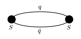
Figure 1: The scalar $q\bar{q}$ Green’s function $G_{q\bar{q}}$

Here $s$ is the external current, e.g. in the $f_{0}(500),f_{0}(980)$ cases ($I=0$) it is equal to 1, while $\Lambda$ is the quark propagator, $\Lambda=(\hat{\partial}+m_{q}+M)^{-1}$.

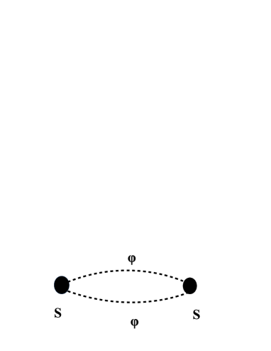
Figure 2: The scalar $\varphi\varphi$ Green’s function $G_{\varphi\varphi}$

At this point we can find the form of the $q\bar{q}$ Green’s function augmented by the transition to the $\phi\phi$ system, which is needed to start the chain of transformations, discussed here. This structure is presented in the next figure.

Figure 3: The scalar $q\bar{q}$ Green’s function with the emission of the chiral mesons

As seen from (8) and following [40], one can find the numerical coefficient $C^{(I)}_{\varphi\varphi}$ in the transition factor $k^{(I)}(q\bar{q}|\varphi\varphi)$, which defines how many ${\varphi\varphi}$ are produced by the one $q\bar{q}$ state. In [40] this was done for isospin $I=0,1$. Here we shall consider also the case of the $K\pi$ channel $(I=1/2$).

We conclude this section with the explicit form of the $I=1/2$ isotopic current, producing $K\pi$ in the case of the $K^{*}_{0}(700)$ resonance.

$$tr\left(j(u\bar{s})\frac{\hat{\varphi}^{2}}{2}\right)=K^{+}\frac{\pi^{0}}{\sqrt{2}}+K^{0}\pi^{+}$$ (9)

$$tr\left(j(d\bar{s})\frac{\hat{\varphi}^{2}}{2}\right)=K^{+}{\pi^{0}}-\frac{\pi^{0}}{\sqrt{2}}K^{0}$$ (10)

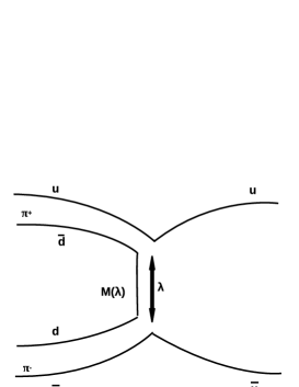
Figure 4: The transition region ($q\bar{q}|\varphi\varphi)$ with the spatial distance $\lambda$ between the constituents

3 Dynamics of the $q\bar{q}$ and the meson-meson systems

The structure of the transition operator $M\frac{\hat{\varphi}^{2}}{2}$ (8) requires a detailed investigation. In [40] it was understood that the free meson-meson Green’s function, created and annihilated at local points, diverges logarithmically and should be replaced by the physically motivated meson-meson Green’s function, where initial and final distances between mesons are defined dynamically, i.e. by the effective distance $\lambda$ from the stationary point of the transition coefficient. In the present paper we shall follow the same line of reasoning and define the meson-meson Green’s function with fixed spatial distance $\lambda$ between the mesons at the initial and final point.

One can start with local $\varphi\varphi$ Green’s function $G_{\varphi\varphi}(x,y)$, created by $\hat{\varphi}^{2}(x)$ in (8), $G_{\varphi\varphi}(P)$ with the total momentum $P=(E,0)$

$$G_{\varphi\varphi}(P)=\frac{1}{(2\pi)^{4}}\int\frac{d^{4}p}{(p^{2}-m^{2}_{1})((P-p)^{2}-m^{2}_{2})}.$$ (11)

To take into account nonlocality in the initial or final vertex we shall examine the structure of this nonlocal vertex in more detail, assuming its structure as shown in Fig. 4. As seen, for the distance $\lambda$ between $q$ and $\bar{q}$ (and effectively between $\varphi$ and $\varphi$) one should have the corresponding Green’s functions $G_{q\bar{q}}$ and $G_{\varphi\varphi}$ of the form $G^{(\lambda)}_{q\bar{q}}(x,x^{\prime}|y,y^{\prime}),G^{(\lambda)}_{\varphi\varphi}(y,y^{\prime}|u,u^{\prime})$ with the distance $\lambda=|\mbox{\boldmath${\rm x}$}-\mbox{\boldmath${\rm x}$}^{\prime}|\cong|\mbox{\boldmath${\rm y}$}-\mbox{\boldmath${\rm y}$}^{\prime}|$. The effective value of $\lambda$ in this vertex $(q\bar{q}|\varphi\varphi)$ is defined by the product $G^{(\lambda)}_{q\bar{q}}\sigma\lambda G^{(\lambda)}_{\varphi\varphi}$ which amounts to the $\lambda$ dependence of the transition coefficient and will be found below in the next sections.

The Green’s function $G^{(\lambda)}_{\varphi\varphi}(y,y^{\prime}|u,u^{\prime})$ can be written as a product $\int\frac{d^{4}p}{(2\pi)^{4}}f(p)\exp(ip(y-u))\int\frac{d^{4}p^{\prime}}{(2\pi)^{4}}f(p^{\prime})\exp(ip^{\prime}(y^{\prime}-u^{\prime})$. Now writing $\exp(i(py+p^{\prime}y^{\prime})=\exp(i(p+p^{\prime})(y+y^{\prime})/2+i(p-p^{\prime})(y-y^{\prime})/2)$ with $P=(p+p^{\prime})$, one can make the Fourier transformation in $(y+y^{\prime})/2$ while integrating over angles of the spatial vector $(y-y^{\prime})$. The same arrangement can be done for $u,\,u^{\prime}$ vectors. Denoting $p-p^{\prime}=q$, one ends up with the same integral eq.(11) , multiplied with the square of the angular integral of $\exp(i\mbox{\boldmath${\rm q}$}\bm{p}\lambda)$.

As it is we need the explicit form of the meson-meson $G^{(\lambda)}_{\varphi\varphi}(yy^{\prime}|uu^{\prime})$ and the $q\bar{q}$ Green’s function $G^{(\lambda)}_{q\bar{q}}(xx^{\prime}|yy^{\prime})$, defined with the initial and final spatial distance $\lambda$ between $\varphi$ and $\varphi$ or $q$ and $\bar{q}$. Since $G^{(\lambda)}_{q\bar{q}}$ is convergent at $\lambda=0$, we shall consider this effect later in this section and now start with the effect of spatial distance $\lambda$ in $G^{(\lambda)}_{\varphi\varphi}$. As shown above, the latter amounts to the angular integration of the factors $\exp(ip(u-u^{\prime}))$ and $\exp(ip(y-y^{\prime}))$, where we denote $q=p$.

The result can be written in the form of the additional factor $F(\lambda p)=\left(\frac{\sin(\lambda p)}{\lambda p}\right)^{2},$ $p=|\bm{p}|$, appearing in (11), namely,

$$G^{(\lambda)}_{\varphi\varphi}(P)=\frac{1}{(2\pi)^{4}}\int\frac{d^{4}pF(\lambda p)}{(p^{2}-m^{2}_{1})\left((P-p)^{2}-m^{2}_{2}\right)},$$ (12)

where $F(\lambda p)=\left(\frac{\sin(\lambda p)}{\lambda p}\right)^{2},~{}~{}p=|\bm{p}|$, appears due to averaging over directions of $\Delta\mbox{\boldmath${\rm y}$}=\mbox{\boldmath${\rm y}$}-\mbox{\boldmath${\rm y}$}^{\prime}$, $\Delta\mbox{\boldmath${\rm u}$}=\mbox{\boldmath${\rm u}$}-\mbox{\boldmath${\rm u}$}^{\prime}$, with $|\Delta\mbox{\boldmath${\rm y}$}|=|\Delta\mbox{\boldmath${\rm u}$}|=\lambda$.

The explicit form of (12) can be written in the c.m. frame,

$$\operatorname{Re}G^{(\lambda)}_{\varphi\varphi}(E)=\int^{\infty}_{0}\frac{p^{2}dp}{4\pi^{2}}\frac{F(\lambda p)}{\sqrt{p^{2}+m^{2}_{1}}\sqrt{p^{2}+m^{2}_{2}}}\times$$

$$\times\left\{\frac{E(\sqrt{p^{2}+m^{2}_{1}}+\sqrt{p^{2}+m^{2}_{2}})+m^{2}_{1}-m^{2}_{2}}{\left[(\sqrt{p^{2}+m^{2}_{1}}+\sqrt{p^{2}+m^{2}_{2}})^{2}-E^{2}\right]\left[E+\sqrt{p^{2}+m^{2}_{1}}-\sqrt{p^{2}+m^{2}_{2}}\right]}\right\}$$ (13)

$$\operatorname{Im}G^{(\lambda)}_{\varphi\varphi}(E)=\frac{F(\lambda p_{0})}{16\pi}\frac{\sqrt{[E^{2}-(m_{1}+m_{2})^{2}][E^{2}-(m_{1}-m_{2})^{2}]}}{E^{2}},$$ (14)

where $p_{0}$ is found from the relation $\sqrt{p^{2}_{0}+m^{2}_{1}}+\sqrt{p^{2}_{0}+m^{2}_{2}}=E\geq m_{1}+m$. Another way of the renormalization of $\operatorname{Re}G_{\varphi\varphi}(E)$ was accepted in [40], with $F(\lambda p)\to 1$ and the fixed upper limit of the $p$ integration, $p\leq N=1/\lambda$. In what follows we shall compare both ways and find that they produce similar results. It is clear that the factor $F(\lambda p)$ is not introduced by hand, but results from the S-wave angular integration of the product of the two-meson Green’s functions at the spatial distance $\lambda$ from each other, which does not give rise to additional singularities. Note that $F(\lambda p)$ is actually a function of $\lambda^{2}p^{2}$ and therefore it does not contribute to the difference $G_{\varphi\varphi}^{(\lambda)}(E+i\delta)-G^{(\lambda)}_{\varphi\varphi}(E-i\delta)$ on the cut $E\geq m_{1}+m_{2}$, and hence does not violate the unitarity condition.

In the case of the $K\pi$ Green’s function one has $m_{1}=m_{K}$ (493 MeV for $K^{\pm}$), and $m_{2}=m_{\pi}\cong 140$ MeV. The resulting form (13) of the $\operatorname{Re}G^{(\lambda)}_{\pi K}(E)$ was computed numerically in the range 640 MeV $\leq E\leq 1200$ MeV for $\lambda=(0.5;1;2;3)$ GeV^-1. The results of calculations show that $\operatorname{Re}G^{(\lambda)}_{\pi K}(E)$ is almost constant in the range $[0.64\div 0,9]$. For the following we shall need the values of $\operatorname{Re}G^{(\lambda)}_{\pi K}$ at the point $E=0.64$ GeV and 0.8 GeV, given in Table 1.

Table 1: The real part of the $K\pi$ Green’s function as a function of the spacial distance $\lambda$ for two values of the energy, $E=640$ MeV and$E=800$ MeV

$\lambda$ (GeV-1	$\operatorname{Re}G^{(\lambda)}_{\pi K}$ (640 MeV)	$\operatorname{Re}G^{(\lambda)}_{\pi K}$ (800 MeV)	$\operatorname{Re}G^{(\lambda)}_{\pi K}$ (640 MeV, cut-off)
0.5	0.033	0.028	0.03
1	0.025	0.02	0.022
1.5	0.02	0.0165	0.017
2	0.017	0.013	0.013
3	0.013	0.007

In the right column of Table 1 the values of $\operatorname{Re}G^{(\lambda)}_{\pi K}(E=640$ MeV) are obtained with the cut-off of the integral over $dp$ in (13) at $N=1/\lambda$. One can see their close values, within (10-15)% accuracy, in the columns 1 and 3.

Now we turn to the $q\bar{q}$ Green’s function and shall use the same formalism for the $(n\bar{s})$ system, as in [40] for the $(n\bar{n})$ system; for that one can exploit calculated positions of the $(n\bar{n})$ pole (see Table 2) and analogously, the $(s\bar{s})$, and $n\bar{s}$ poles. To calculate the $q\bar{q}$ Green’s function and the $q\bar{q}$ eigenvalues we use, as in [40], the exact relativistic formalism (see [59] for a review and references, based on the Field Correlator Method [60]). This yields the relativistic Hamiltonian in the c.m. frame, containing the quark and antiquark kinetic energies $\omega_{1},\omega_{2}$,

$$H(\omega_{1},\omega_{2},\bm{p})=\sum_{i=1,2}\frac{\bm{p}+\omega_{i}^{2}+m^{2}_{i}}{2\omega_{i}}+V_{0}(r)+V_{s0}(r)+V_{t}$$ (15)

Now one has two options to define $\omega_{i}$: 1) to minimize $H(\omega_{1},\omega_{2},\bm{p})$ in the values of $\omega_{1},\omega_{2}$, which leads to the so-called Spinless Salpeter Equation (SSE), widely used (see e.g. [36]), or to calculate the eigenvalue of (14) $E(\omega_{1},\omega_{2})$ and then to find its minimum (so-called the “einbein approximation” $(EA$); see [37, 39, 59] for details). The comparison of these approximations for the cases of $n\bar{n}$ scalar meson masses is given in Table  2.

The interaction terms $V_{0},V_{so},V_{t}$ are the instantaneous potentials of the scalar confinement $V_{0}$, perturbative and nonperturbative spin-orbit interactions $V_{s0}$, and tensor interaction $V_{t}$, which define the center-of-gravity eigenvalue $M_{\rm cog}(nP)$, the spin-orbit correction $a_{\rm so}(nP)$, and the tensor correction $c_{t}(nP)$. For the masses of the $n^{3}P_{0}$ states one has [37, 39]

$$M(n^{3}P_{0})=M_{\rm cog}(n^{3}P_{0})-2a_{\rm so}-c_{t}.~{}$$ (16)

The resulting masses of the $n\bar{n}$, $n\bar{s},s\bar{s}$ states are given in the Table  2

Table 2: The masses (in MeV) of the $1^{3}P_{0}$ and $2^{3}P_{0}$ $n\bar{n}$ states, obtained in the SSE, EA and RT (the Regge trajectory formalism) by Badalian and Bakker [37, 39], Ebert et. al. [38], and Godfrey, Isgur [36]

State	BB [37, 39]			EFG [38]	GI [36]
	SSE	EA	RT
$n\bar{n}~{}1^{3}P_{0}$	1050	1093	1038	1176	1090
$2^{3}P_{0}$	1461	1594	1435	1679	1780

As shown in [59, 60] the $q\bar{q}$ Green’s function can be written as a sum over the pole terms. As in [40], the lowest pole contribution to the $(q\bar{q})$ Green’s function $G_{q\bar{q}}(E)$ can be written as

$$G_{q\bar{q}}(E)=\sum^{\infty}_{n=1}\frac{(f^{(n)}_{s})^{2}M^{2}_{n}}{M^{2}_{n}-E^{2}}=\frac{(f_{s}^{(1)})^{2}M^{2}_{1}}{M^{2}_{1}-E^{2}}+...$$ (17)

where $f_{s}^{(1)}$ was calculated in the $(n\bar{n})$ case in [40], while for all $q\bar{q}$ states it is given in Appendix A1, and within the 10% accuracy it has the value, $f^{(1)}_{s}\cong 100$ MeV, whereas the mass $M_{1}(n\bar{s})$ is obtained to be $M_{1}=(1210\div 1240)$ MeV, and $M_{1}(s\bar{s})\cong 1400$ MeV, see Table  3.

Table 3: The masses (in MeV) of the $n^{3}P_{0}$ $q\bar{q}$ scalars, obtained in the method of [37, 39], and their experimental values in the $\pi\pi,K\bar{K},\,\pi\eta,\,\pi K$ systems

$n_{r}$		$n\bar{n}(I=1)$	$n\bar{n}(I=0)$	$n\bar{s}\left(I=\frac{1}{2}\right)$	$s\bar{s}(I=0)$
	$M_{1}$	1.050	1050	1240	1400
0	exp	$a_{0}(980)$	$f_{0}(980),f_{0}(500)$	$K^{*}_{0}(700)$	$\tilde{f}_{0}(1370)$
	$M_{2}$	1500	1500	1550	1740
1	exp	$a_{0}(1450)$	$f_{0}(1500)$	$K^{*}_{0}(1430)$	$\tilde{f}_{0}(1710)$

Now we can write the final equation for the position of the pole, resulting from the infinite series of the $(q\bar{q})\to(\varphi\varphi)\to(q\bar{q})\to...$ transformations, in the same way as it was done in [40].

$$E^{2}=M^{2}_{1}\left\{1-k^{(I)}(q\bar{q}|\varphi\varphi)(\operatorname{Re}G^{(\lambda)}_{\varphi\varphi}(E)+i\operatorname{Im}G^{(\lambda)}_{\varphi\varphi}(E))\right\},$$ (18)

where

$$k^{(I)}(q\bar{q}|\varphi_{1}\varphi_{2})=\frac{C^{2}_{i}M^{2}(\lambda)(f_{s}^{(1)})^{2}}{f^{2}_{\varphi_{1}}f^{2}_{\varphi_{2}}}.$$ (19)

At this point it is interesting to discuss the position of the poles, which are the self-consistent solutions of the (18). To start we consider the simplest case with equal masses of two mesons, $m_{1}=m_{2}$ and $E^{2}=p^{2}+4m^{2}$, and start, solving the equation (18) in terms of the variable $p$, taking into account that $\operatorname{Re}G$ is the constant and $\operatorname{Im}G$ is proportional to $p$, $\operatorname{Im}G=pf(p^{2})$. As a result one obtains the equation for the position of the resonance in terms of $p$:

$$p^{2}+ipf(p^{2})-p_{0}^{2}=0.$$ (20)

As a first approximation one can take $f(p^{2})=f(p_{0}^{2})=f_{0}$ and solving the quadratic equation, one obtains

$$p=-if_{0}/2+/-sqrt{(f_{0})^{2}/4+p_{0}^{2}},$$ (21)

which explicitly shows that the pole is on the second sheet with respect to the $2m$ threshold. In next approximations one takes into account, step by step, the $p$ dependence of $f(p^{2})$, observing the motion of the pole on the second sheet.

In Eq. (19) $C^{2}_{i}$ can be found for the $\pi\pi,K\bar{K},\pi\eta$ cases as in [40] and from (9), (10), and for $\pi K$ system it is equal to

$$C^{2}_{i}=\left(1+\frac{1}{\sqrt{2}}\right)^{2}=\frac{3}{2}+\sqrt{2}=2.91\approx 3,$$ (22)

while the PS decay constants $f_{i}$ are known from [53], experimental and lattice data,

$$f_{K}=111~{}{\rm MeV}~{},f_{\pi}=93~{}{\rm MeV}~{},f_{\eta}=120~{}{\rm MeV}~{}.$$ (23)

The quark decay constants of the scalar mesons $f_{s}^{(i)}$ are calculated via the radial derivative of the $q\bar{q}$ wave function, as shown in Appendix A1, with the values given in Table 8. In Appendix A2 we show that $f_{s}^{i)}$ are strongly dependent on the value of $\lambda$ and the effective region of $\lambda$ is inside the range $0\leq\lambda\leq 1.5$ GeV^-1. At the same time another factor in (19) $M^{2}(\lambda)$ grows with $\lambda$, so that the optimal values of $\lambda$ can be obtained from the ratio $\frac{k^{(I)}(q\bar{q}|\varphi\varphi)}{k^{(I)}_{\max}(q\bar{q}|\varphi\varphi)}\equiv X(\lambda)$, given in Table 4

Table 4: The dependence of the ratio of the transition factor $k^{I}(q\bar{q}|\varphi\varphi)/k^{(I)}_{\max}$ on the spatial contact distance $\lambda$.

$\lambda$ (GeV${}^{-1})$	0.5	1	1.5	2
$X(\lambda)$	0.29	0.816	1	0.04

Then taking into account that $M(\lambda)=\sigma\lambda=0.18$ GeV${}^{2}\cdot\lambda$, one has the following values of the transition factors $k^{(I)}(q\bar{q}|\varphi\varphi)$ at $\lambda=1$ GeV^-1 and $\lambda=1.5$ GeV^-1 (see Table 5).

Table 5: The transition factor $k^{(I)}(q\bar{q}|\varphi\varphi)$ at $\lambda=1$ GeV^-1 and $\lambda=1.5$ GeV^-1 for different channels

$k(q\bar{q}|\varphi\varphi)$	$(n\bar{n}|\pi\pi)$	$(n\bar{n}|KK)$	$(n\bar{n}|\pi\eta)$	$(n\bar{s}|\pi K)$	$(s\bar{s}|KK)$
$\lambda=1$ GeV-1	18.44	4.02	3.0	14.2	3.0
$\lambda=1.5$ GeV-1	41.51	9.05	6.72	31.2	6.75

Using these values of $k^{(I)}(\bar{q}\bar{q}|\varphi\varphi)$ in Eq. (18) and the values of $M_{1}$ from Table 3, one obtains the parameters of the resonances in the channels $\pi\pi,KK,\pi\eta$ $\pi K$, given in Table 6.

Table 6: The resonances in the channels $\pi\pi,K\bar{K},\pi\eta,\pi K$, coupled at the distance 1 GeV^-1 and $\lambda=1.5$ GeV^-1 to the $q\bar{q}$ poles $(n\bar{n},n\bar{s},s\bar{s})$, in comparison with experimental PDG data

	$(q\bar{q}|\varphi\varphi)$	$(n\bar{n}|\pi\pi)$	$(n\bar{n}|K\bar{K})$	$(n\bar{n}|\pi\eta)$	$(n\bar{s}|\pi K)$	$(s\bar{s}|K\bar{K})$
	$k(q\bar{q}|\varphi\varphi)$	18.44	4.02	3.0	14.2	3.0
$\lambda=1$	$\operatorname{Re}G_{\varphi\varphi}$	0.02	0.011	0.02	0.025	0.011
	$\operatorname{Im}G_{\varphi\varphi}$	0.015	0.02	0.015	0.015	0.02
	$\operatorname{Re}a,\operatorname{Im}a$	0.38;0.276	0.045+i0.08	0.06+i0.045	0.36+ i0.213	0.033+i0.06
	$E$	0.85-i0.17	1.025-i0.044	1.02-i0.025	0.714-i0.078	1.37-i0.041
	$k(q\bar{q}|\varphi\varphi)$	41.51	9.05	6.75	31.2	6.75
$\lambda=1.5$	$\operatorname{Re}G_{\varphi\varphi}$	0.015	0.018	0.018	0.0165	0.018
	$\operatorname{Im}G_{\varphi\varphi}$	0.0155	0.015	0.015	0.015	0.015
	$\operatorname{Re}a,\operatorname{Im}a$	0.645;0.645	0.162+i0.136	0.1215+i0.10	0.52+ i0.468	0.12+i0.10
	$E$	0.64-i0.54	0.966-i0.08	0.98-i0.056	0.75-i0.21	1.31-i0.074
	$E_{PDG}$	0.400-0.550	0.990	0.980	0.630-0.730	1.200-1.500
	$\Gamma_{PDG}$	0.400-0.700	0.010-0.100	0.050-0.100	0.478(50)	0.200-0.500

From Table 6 one can see that suggested the pole projection mechanism (PPM) yields a reasonable picture of the resulting resonances in all $\varphi\varphi$ channels, and the differences between calculated and observed resonance characteristics $(R,\Gamma)$ are of the order of indeterminacy intervals. A possible sign of disagreement seems to be in the $f_{0}(500)$ resonance, where PPM gives a resonance position some 150-200 MeV above the experimental value. As it was discussed in [40], this fact implies that the $\pi\pi$ interaction in the $\pi\pi$ Green’s function, $G_{\pi\pi}(E)$, has to be used to account for the low energy region, $E\mathrel{\mathchoice{\lower 3.6pt\vbox{\halign{$\mathsurround=0pt\displaystyle\hfil#\hfil$\cr<\crcr\sim\crcr}}}{\lower 3.6pt\vbox{\halign{$\mathsurround=0pt\textstyle\hfil#\hfil$\cr<\crcr\sim\crcr}}}{\lower 3.6pt\vbox{\halign{$\mathsurround=0pt\scriptstyle\hfil#\hfil$\cr<\crcr\sim\crcr}}}{\lower 3.6pt\vbox{\halign{$\mathsurround=0pt\scriptscriptstyle\hfil#\hfil$\cr<\crcr\sim\crcr}}}}500$ MeV. Indeed, the accurate analysis in [61] confirms the $f_{0}(500)$ pole position at $E=(457-i279)$ MeV, close to $E_{\exp}$. If this interaction is neglected, from Table 6 for $\lambda=(1,1.5)$ GeV^-1 we have

$$E({\rm GeV})=(0.85\div 0.64)-i(0.17\div 0.54),$$ (24)

which differs from $E_{exp},$ while the $f_{0}(980)$ data is comparable to our result.

4 The case of two $q\bar{q}$ poles

Till now we have studied the lowest ${}^{3}P_{0}$ quark-antiquark poles, which due to the PPM are shifted down from the original position of around (1000$-1400)$ MeV to the final position in the range (700-1300) MeV, which can be associated with the lowest exotic resonances. However, in the ($n\bar{n})$ channel there is the radially excited pole $0^{++},I=0$ at the initial position $M_{1}=(1490-1500)$ MeV, which can be also shifted down and have the position around 1400 MeV, known as $f_{0}(1500)$. Also in the $K_{0}^{*}$-channel ($J^{PC}=0^{++},I=\frac{1}{2}$) there exists the higher resonance, coupled to the same $K\pi$ decay channel, $K_{0}^{*}(1430)$, which can be originated from the radial excited $(n\bar{s})$ pole at $M_{2}=1550$ MeV. Below we shall show a remarkable property of the PPM, where the shift down of the lowest $(q\bar{q})$ pole changes a little, if the radial excitations are taken into account, while the mass shift of the higher $(q\bar{q})$ pole is strongly suppressed as compared to the ground state. This property of the level repulsion follows from the structure of the PPM equations themselves.

Indeed, writing the one-channel, one-pole PPM Eq.(35) in the form as in [40], one has

$$G_{\varphi\varphi}(E)k^{(I)}(q\bar{q}|\varphi\varphi)\frac{M^{2}_{1}}{M^{2}_{1}-E^{2}}=1,$$ (25)

with

$$k^{(I)}(q\bar{q}|\varphi\varphi)=\frac{(C_{\varphi\varphi}^{(I)})^{2}M^{2}(\lambda)(f^{(1)}_{s})^{2}}{f_{\varphi}^{4}},~{}~{}f_{\varphi}=f_{\pi},f_{K},f_{\eta}$$ (26)

This equation can be generalized, including the radially excited pole $M_{2},$ as follows

$$G_{\varphi\varphi}(E)\left[k^{(I)}_{1}(q\bar{q}|\varphi\varphi)\frac{M^{2}_{1}}{M^{2}_{1}-E^{2}}+k^{(I)}_{2}(q\bar{q}|\varphi\varphi)\frac{M^{2}_{2}}{M^{2}_{2}-E^{2}}\right]=1$$ (27)

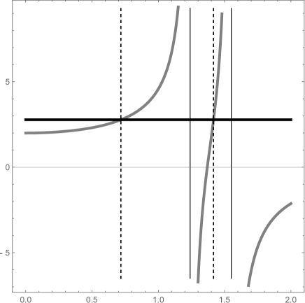
Figure 5: The function $f(E)$ is shown by thick grey lines, with two poles at $E=M_{1},M_{2}$ (shown by thin vertical lines). The intersections of $f(E)$ with the horizontal line at $a^{-1}=1/0.36$ yields two resulting poles $E=E_{1},E_{2}$, marked by vertical dashed lines

To understand better the situation with two projected poles we consider the Eq.(27) and approximate $k_{1}^{(I)}\approx k_{2}^{(I)}$ (which holds in most cases according to Table  8 in Appendix A1). From (27) one has the equation

$$f(E)=\frac{M^{2}_{1}}{M^{2}_{1}-E^{2}}+\frac{M^{2}_{2}}{M^{2}_{2}-E^{2}}=\frac{1}{k^{(I)}G_{\varphi\varphi}(E)}=a^{-1},$$ (28)

Then taking the case $(n\bar{s}|\pi K)$ as an example and neglecting $\operatorname{Im}G_{\varphi\varphi}$, from Table 6 one obtains $a=k^{(1/2)}\operatorname{Re}G_{\pi K}=0.36$, and the resulting $f(E)$, as a function of $E$, has two poles, defined by the intersection of the straight line $f(E)=\frac{1}{0.36}$ (see Fig. 5). From Fig. 5 one can easily see how the resulting poles $E_{1},E_{2}$ are shifted as compared to $M_{1},M_{2}$, in the approximation of zero $\operatorname{Im}G_{\pi K}$.

To proceed with the case of $K^{*}_{0}(700),K^{*}_{0}(1430)$, we are solving the quadratic in $E^{2}$ equation (28) with $M_{1}=1.24,~{}~{}M_{2}=1.55$ GeV, and obtain two approximate solutions for $\lambda=1$  GeV^-1

$$E_{1}=(0.78-i~{}0.33)~{}{\rm GeV},~{}~{}E_{2}=(1.40-i~{}0.035)~{}{\rm GeV}.$$ (29)

These solutions correspond to the intersection points in Fig.5 and were obtained treating the imaginary part of $G_{\pi K}(E)$ as perturbation. To take it fully into account one can write the solution of (28) as

$$E^{2}=\frac{1}{2}(M^{2}_{1}+M^{2}_{2})(1-a)\pm\sqrt{\frac{1}{4}(M^{2}_{1}+M^{2}_{2})^{2}(1-a)^{2}-M^{2}_{1}M^{2}_{2}(1-2a)}$$ (30)

and use

$$a=\operatorname{Re}a+i\operatorname{Im}a=k^{(I)}(q\bar{q}|\varphi\varphi)(\operatorname{Re}G_{\varphi\varphi}+i\operatorname{Im}G_{\varphi\varphi})$$

from the Table 6 in the case $(n\bar{s}|\pi K)$, calculated e.g. for $\lambda=1$ GeV^-1.

In a similar way one can consider all the cases: $(n\bar{n}|\pi\pi),$ $(n\bar{n}|K\bar{K}),$ $(n\bar{n}|\pi\eta),$ $(n\bar{s}|K\pi)$ and $(s\bar{s}|K\bar{K})$. The resulting pole positions for $\lambda=1$ GeV^-1, generated by ground and radially excited scalar $q\bar{q}$ poles, are given in the Table 7.

Table 7: The scalar resonance positions and the widths in the two-pole formalism

The $(q\bar{q}|\varphi\varphi)$ connection	$(n\bar{n}|\pi\pi)$	$(n\bar{n}|K\bar{K})$	$(n\bar{n}|\pi\eta)$	$(n\bar{s}|\pi K)$	$(s\bar{s}|K\bar{K})$
$n_{r}=0$	1.05	1.05	1.05	1.24	1.4
The $q\bar{q}$ mass (GeV)
$n_{1}=1$	1.50	1.5	1.5	1.55	174
Transition coefficient	18.44	4.02	3.0	14.2	3.0
$k^{(I)}(q\bar{q}|\varphi\varphi)$
$a(E)=k^{(I)}G_{\varphi\varphi}(E)$	0.38+i0.28	0.045+i0.08	0.06+i0.045	0.36+i0.213	0.033+i0.06
$E_{1}(n_{r}=0)$ (GeV),	0.8	1.04	1.02	0.85	1.36
$\Gamma_{1}$(MeV)	980	32	40	640	72
	$f_{0}(500)$	$f_{0}(980)$	$a_{0}(980)$	$K_{0}^{*}(700)$	$f_{0}(1370)$?
$E^{(1)}_{PDG}$ (GeV)	0.40-0.55	0.99	0.98	0.63-0.73	1.2 $\div 1.5$
$\Gamma_{PDG}$ (MeV)	400-700	0.10-100	0.50-100	480	200$\div$500
$E_{2}(n_{r}=1)$(GeV)	1.28	1.45	1.45	1.4	1.72
$\Gamma$ (MeV)	100	84	52	40	76
	$f_{0}(1370)$	$f_{0}(1500)$	$a_{0}(1450)$	$K_{0}^{*}(1430)$	$f_{0}(1710)$
$E^{(2)}_{PDG}$	1200-1500	1.50	1.48	1.425	1.72
$\Gamma$ (MeV)	200$\div$500	$\Gamma=109$	$\Gamma=265$	$\Gamma=270$	$\Gamma=120$

From Table 7 one can see a reasonable agreement of predicted and observed resonance characteristics, but with a few exclusions. The first one refers to the higher position of the predicted mass $f_{0}(500)$ with $E_{1}=800$ MeV, however, with a large width, which implies significant uncertainty in the resonance position, and, as we discussed above, calls for the account of the $\pi\pi$ interaction in $G_{\pi\pi}$ at small energies. The second discrepancy might be more significant. Namely, the first $(s\bar{s}|K\bar{K})$ resonance occurs exactly at 1.37 GeV (see Table 7) and could be associated with $f_{0}(1370)$, however, the latter prefers to decay into $\pi\pi,4\pi$ and the $K\bar{K}$ ratio is less than 10% [1].

At the same time the second $(n\bar{n}|\pi\pi)$ resonance is predicted at around 1.3 GeV with the width $\Gamma_{\pi\pi}\approx 100$  MeV, and the $(n\bar{n}|K\bar{K})$ resonance is at 1.45 GeV with the width $\Gamma_{K\bar{K}}\approx 100$ MeV; the latter has to be associated with $f_{0}(1500)$. Unfortunately $f_{0}(1500)$ decays mostly into $\pi\pi,4\pi$. Thus one faces three inconsistencies in the theory: $\pi\pi$ resonance at 1300 MeV and two $K\bar{K}$ resonances at 1450 MeV and 1360 MeV, while in experiment one has two resonances $f_{0}(1370)$ and $f_{0}(1500)$, decaying mostly into $\pi\pi$ and $4\pi$.

Evidently, here appears a strong mixing pattern of three (or more) resonances, which can be additionally enlarged by the code mechanism $(K\bar{K}|n\bar{n})\frac{M_{2}}{M^{*}_{2}-E^{2}}(n\bar{n}|\pi\pi)$ near the $n\bar{n}$ pole at $M_{2}=1.5$ GeV. As an additional argument for this mixing and the resulting damping of the $K\bar{K}$ decay mode, one can use the small value of the $K\bar{K}$ decay width of 70 MeV for the $(s\bar{s}|K\bar{K})$ resonance at 1.36 GeV, while corresponding experimental resonance $f_{0}(1370)$ has a large $\pi\pi,4\pi$ width, $\Gamma=(200\div 500)$ MeV. This interesting topic requires a substantial analysis and a separate publication.

5 Conclusions and an outlook

In our paper we presented the simplest version of the channel coupling (CC) mechanism with the code – $(q\bar{q}|\varphi\varphi)$, which is the relativistic and the chiral extension of original the Cornell code, used for the charmonium resonances [41]. This is the realization of the CC mechanism [44], where due to infinite set of transformations of one system into another one can provide a pole (the bound state) in this set, even if both systems are free. Here the basic role is played by the magnitude of the transition amplitude and the concrete example of the resulting $Z_{b}$ resonances was given in the last refs. of [43].

It was also demonstrated that in the case of scalar mesons the role of transition coefficient $k^{(I)}(q\bar{q}|\varphi\varphi)$ is extremely important, since it can be very large number, $(k^{(0)}(n\bar{n}|\pi\pi)=O(18-40))$ in the $(n\bar{n}|\pi\pi)$ and the $(n\bar{s}|K\pi)$ cases (see Table 6), and small, $(k=O(1))$, in other cases. In Tables 6 and 7 one can see that just this large range of the changes helps to understand the situation with the scalar mesons, where the shifts of the resonances are so different in different $\varphi\varphi$ systems, and the maximal one is in the $(n\bar{n}|\pi\pi)$ case.

At this point one can see the main difference of the present approach from other existing formalisms. As was explained in the paper, the connection between $q\bar{q}$ and the meson-meson channels plays the basic role and starting from the single $q\bar{q}$ pole, one can define the parameters of all lowest scalar resonances (this does not mean that other mechanisms are ruled out). However, here one must find the transition coefficients explicitly, without fitting parameters, which we could do with the use of the CCL and the stationary point in the function $k^{(I)}(\lambda)$. An approximate way of adjusting this connection was already used in the unitarized meson model [19, 20, 21], where one needs to introduce two to three parameters to describe the transitions. Another approach is the dispersive method [61], where the rigorous integral equations are used in comparison with data. At this point we should stress that the final adjustment of the positions of the lowest scalar resonances, obtained in our formalism without fitting parameters, nevertheless, requires the use of these results, as was demonstrated in [40], where the data of [61] were essentially used.

Another important feature of the PPM is the appearance of the resonance, created by a single $q\bar{q}$ pole – the resulting $\varphi\varphi$ resonance can appear, in principle, in each $\varphi\varphi$ system, connected to this $q\bar{q}$ pole. To have more resonances, connected to the same $q\bar{q}$ pole, one needs additional direct $\phi_{1}\phi_{1}$-$\phi_{2}\phi_{2}$ interaction. This happens for $\pi\pi$ and $K\bar{K}$ systems, where two resonances $f_{0}(500)$ and $f_{0}(980)$ are created in this way by the $q\bar{q}$ pole at $E=1050$ MeV. Note, that finally these resonances become connected due to the $\pi\pi-K\bar{K}$ channel coupling, and in some cases two close-by resonance poles can be located on different sheets, as was observed in lattice analysis by J. Dudek et al. [18].

We have already stressed the important role of the $\varphi\varphi$ interaction in obtaining the correct position of lowest resonances $f_{0}(500)$ and $K^{*}_{0}(700)$. Actually our approach provides an alternative way for the description of the $\varphi\varphi$ scattering amplitudes, when the $q\bar{q}$ dynamics is included at the first stage, and the $q\bar{q}-\varphi\varphi$ transition is taken into account as a second step, and the final stage should include the detailed account of the $\varphi\varphi$ interaction. The comparison of the resulting $\pi\pi$ amplitude, using only two first steps, with the realistic $\pi\pi$ data, done in [40], exactly shows that the two-step amplitude roughly describes main features - the extrema and zeros of the amplitude, but strongly distorts the amplitude at small energies, where the $\varphi\varphi$ interaction is important. To solve the scalar meson problem, as it was demonstrated above, the simplified two-step procedure was sufficient. On another hand, the full three-step procedure provides the exact $\varphi\varphi$ amplitude with the correct $q\bar{q}$ input, as it was shown in [40].

Another feature of the PPM, found in this paper, is the relatively smaller shifts of all radial excited resonances, compared to the ground states, especially in the $(n\bar{n}|\pi\pi)$ and $(n\bar{s}|\pi K)$ cases. As a whole, we have explained the general features of the scalar meson spectrum, leaving the details of the $K\bar{K}-\pi\pi$ coupling to the future publications.

The work of two of the authors (M.L. and Yu.S.) is supported by the Russian Science Foundation in the framework of the scientific project, Grant 16-12-10414.

Appendix A1. Decay constants of the $n\bar{n}$, $n\bar{s}$ and $s\bar{s}$ states

As it was explained in [40], the $q\bar{q}$ Green’s function is computed in the Fock-Schwinger formalism, based on the relativistic path integral method. In this formalism the $q\bar{q}$ Green’s function in the c.m. frame $(\mbox{\boldmath${\rm P}$}=0)$ has the form

$$G_{q\bar{q}}(E)=\sum_{n}\frac{(f_{s}^{(n)})^{2}M^{2}_{n}}{M^{2}_{n}-E^{2}}\to\frac{(f_{s}^{(1)})^{2}M^{2}_{1}}{M^{2}_{1}-E^{2}}+\frac{(f_{s}^{(2)})^{2}M^{2}_{2}}{M^{2}_{2}-E^{2}},$$ (A1.1)

where $M_{n},n=1,2,$ are the energy eigenvalues, while $f_{s}^{(n)}$ are the $P$-wave decay constants, which are discussed and calculated in the Appendix 1 of [40].

Here we only detalize the explicit form of $f_{3}^{(1)}$ and its dependence on the quark masses and the radial quantum number $n$. The explicit form of $f_{s}^{(n)}$ can be writen as [40]

$$(f_{s}^{(n)})^{2}=\frac{2N_{c}(R^{\prime}_{nP}(0))^{2}}{4\pi\omega_{n}\bar{\omega}_{n}M_{n}},$$ (A1.2)

where $\omega_{n},\bar{\omega}_{n}$ are the average energies of the quark and the antiquark in the relativistic $q\bar{q}$ system obeyed by the confinement, the color Coulomb and spin-dependent interactions [39]. The concrete calculations, done in this framework as in [40], bring the following results presented in the Table 8.

Table 8: The quark kinetic energy $\omega_{i}$ (in GeV), the derivative of the radial wave function at the origin $R^{\prime}_{iP}(0)$, the masse $M_{i}$ (in GeV), and the decay constant $f_{s}^{(i)}$ for the ground state ($i=1$) and the first excited state ($i=2$)

$q\bar{q}$	$\omega_{1};\omega_{2}$	$R^{\prime}_{1P}(0)$	$R^{\prime}_{2P}(0)$	$M_{1}$	$M_{2}$	$(f_{s}^{(1)})^{2}$	$(f_{s}^{(2)})^{2}$
		(GeV5/2)	(GeV5/2)			(GeV2)	(GeV2)
$n\bar{n}$	0.48; 0.50	0.0845	0.0906	1.05	1.5	0.0142	0.0103
$n\bar{s}$	0.53; 0.56	0.091	0.106	1.24	1.55$\div$1.61	0.010	0.0108
$s\bar{s}$	0.54; 0.57	0.099	0.116	1.4	1.74	0.0112	0.0101

Appendix A2.

As it is shown in (A1.2), the decay constant $f_{s}^{(n)}$ ($s$ - the scalar) is defined via the derivative $R^{\prime}_{nP}(0)$, while other factors in (A1.2) do not depend on $r$.

For the decay constant, defined at the spatial distance $r=\lambda$ between $q$ and $\bar{q}$ (see Fig. 4), the decay constant $f_{s}^{(n)}(\lambda)$ is determined via the derivative $R^{\prime}_{nP}(\lambda)$, i.e. generalizing Eq.(A1.2),

$$(f_{s}^{(n)}(\lambda))^{2}=\frac{2N_{c}(R^{\prime}_{nP}(\lambda))^{2}}{4\pi\omega_{n}\bar{\omega}_{n}M_{n}}$$ (A2.1)

The values of $R^{\prime}_{nP}(\lambda)$ have been computed numerically in the relativistic formalism of [37, 39] and corresponding values of $R^{\prime}_{1P}(\lambda),(R^{\prime}_{1P}(\lambda))^{2}$ are given in the Table 9 together with the ratios of the decay constants $\eta(\lambda)=\left|\frac{f_{s}(\lambda)}{f_{s}(0)}\right|^{2}$

Table 9: The space distances $\lambda$, the derivative of the wave function $R^{\prime}_{1P}(\lambda)$ and $(R^{\prime}_{1P}(\lambda))^{2}$, and the parameter $\eta(\lambda)$ for the ground $n\bar{n}$ state

$\lambda$ (GeV-1)	0.25	0.50	0.75	1.0	1.25	1.50	1.75	2.0
$R^{\prime}_{nP}(\lambda)$ (GeV5/2)	0.0852	0.082	0.0764	0.0684	0.06	0.0504	0.0101	0.0077
$(R^{\prime}_{nP}(\lambda))^{2}$ GeV5	0.00726	0.00672	0.00583	0.00468	0.0036	0.0025	0.0001	5.9$\cdot 10^{-5}$
$\eta(\lambda)=\left|\frac{f_{s}^{(1)}(\lambda)}{f_{s}^{(1)}(0)}\right|^{2}$	0.98	0.91	0.79	0.63	0.486	0.343	0.0138	0.008

References

- [1] M. Tanabashi, K. Hagiwara, K. Hikasa, et al. (Particle Data Group), Phys. Rev. D 98, 030001 (2018).
- [2] N. Brambilla, S. Eidelman, C. Hanhart, et al., arXiv:1907.07583 [hep-ex].
- [3] N. A. Törnqvist, Z. Phys. C 68, 647 (1995), hep-ph/9504372 .
- [4] F. E. Close and N. A. Törnqvist, J. Phys. G 28, 249 (2002), hep-ph/0204205.
- [5] D. V. Bugg, Phys. Rept. 397, 257 (2004), hep-ex/0412045.
- [6] C. Amsler and N. A. Törnqvist, Phys. Rept. 389, 61 (2004).
- [7] R. L. Jaffe, Phys. Rept. 409, 1 (2005), hep-ph/0409065.
- [8] M. R. Pennington, Int. J. Mod. Phys. A 21, 747 (2006), hep-ph/0509265.
- [9] E. Klempt and A. Zaitsev, Phys. Rept. 454, 1 (2007); arXiv:0708.4016 [hep-ex].
- [10] N. N. Achasov, Phys. Usp., 41, 1149 (1998) [hep-ph/9904223]; N. N. Achasov, Nucl. Phys. A 675, 279 (2000), hep-ph/9910540.
- [11] J. R. Pelaez, Phys. Rept. 658, 1 (2016), arXiv:1510.00653 [hep-ph].
- [12] G. Rupp and E. van Beveren, Acta Phys. Polon. Supp 11, 455 (2018), arXiv:1806.00364 [hep-ph].
- [13] N. N. Achasov and G. N. Shestakov, Phys. Usp. 62, 3 (2019), arXiv:1905.11729 [hep-ph].
- [14] R. L. Jaffe, Phys. Rev. D 15, 267 (1977); R. L. Jaffe, Phys. Rev. D 15, 281 (1977); G.’t Hooft, G. Isidori, L. Maiani, et al., Phys. Lett. B 662, 424 (2008), arXiv:0801.2288 [hep-ph]; D. Ebert, R. N. Faustov, and V. O. Galkin, Eur. Phys. J. C 60, 273 (2009), arXiv:0812.2116 [hep-ph]; G. Eichmann, C. Fischer, and W. Heupel, Phys. Lett. B 753, 282 (2016), arXiv:1508.07178 [hep-ph].
- [15] G. Colangelo, J. Gasser, and H. Leutwyler, Nucl. Phys. B 603, 125 (2001), hep-ph/0103088; I. Caprini, G. Colangelo, H. Leutwyler, Phys. Rev. Lett. 96, 132001 (2006), hep-ph/0512364.
- [16] J. D. Weinstein and N. Isgur, Phys. Rev. Lett. 48, 659 (1982); J. D. Weinstein and N. Isgur, Phys. Rev. D 27, 588 (1983); J. D. Weinstein and N. Isgur, Phys. Rev. D 41, 2236 (1990); J. A. Oller, E. Oset, and A. Ramos, Prog. Part. Nucl. Phys. 45, 157 (2000), hep-ph/0002193; E. Oset, W.-H. Liang, M. Bayar, et al., Int. J. Mod. Phys. E 25, 1630001 (2016), arXiv:1601.03972 [hep-ph]; Yu. S. Kalashnikova and A. V. Nefediev, Phys. Usp. 62, 568 (2019), arXiv:1811.01324 [hep-ph].
- [17] Z. G. Wang, Eur. Phys. J. C 76, 427 (2016) [arXiv: 1507.02131].
- [18] M. G. Alford and R. L. Jaffe, Nucl. Phys. B B 578, 367 (2000), [hep-lat/0001023]; H. Suganuma, K. Tsumura, N. Ishii, and F. Okiharu, Prog. Theor. Phys. Suppl. 168, 168 (2007), arXiv:0707.3309 [hep-ph]; N. Mathur, A. Alexandru, Y. Chen et al., Phys. Rev. D 76, 114505 (2007), hep-ph/0607110; M. Loan, Z. H. Luo and Y. Y. Lam, arXiv: 0907.3609 [hep-lat]; S. Prelovsek and D. Mohler, Phys. Rev. D 79, 014503 (2009), arXiv:0810.1759 [hep-lat]; T. Kunihiro, S. Muroya, A. Nakamura, et al. (SCALAR Collaboration), Phys. Rev. D 70, 034504 (2004), hep-ph/0310312; J. J. Dudek, R. G. Edwards, and D. J. Wilson (Hadron Spectrum Collaboration), Phys. Rev. D 93, 094506 (2016), arXiv:1602.05122 [hep-lat]; D. Darvish, R. Brett, J. Bulava, et al., arXiv:1909.07747 [hep-lat].
- [19] E. van Beveren, T. A. Rijken, K. Metzger, et al. Z. Phys. C 30, 615 (1986), arXiv:0710.4067 [hep-ph].
- [20] E. van Beveren and G. Rupp, Eur. Phys. J. C 22, 493 (2001), hep-ex/0106077.
- [21] E. van Beveren, D. V. Bugg, F. Kleefeld, and G. Rupp, Phys. Lett. B 641, 265 (2006), hep-ph/0606022.
- [22] N. A. Tornqvist and M. Roos, Phys. Rev. Lett. 76, 1575 (1996), hep-ph/9511210.
- [23] N. A. Tornqvist, Z. Phys. C 68, 647 (1995), hep-ph/9504372; N. A. Tornqvist and M. Roos, Phys. Rev. Lett. 76, 1575 (1996), hep-ph/9511210.
- [24] M. Boglione and M. R. Pennington, Phys. Rev. D 65, 114010 (2002), hep-ph/0203149.
- [25] T. Wolkanowski, F. Giacosa, and D. H. Rischke, Phys. Rev. D 93, 014002 (2016), arXiv:1508.00372 [hep-ph].
- [26] J. Oller and E. Oset, Phys. Rev. D 60, 074023 (1999), hep-ph/0610397.
- [27] J. R. Pelaez and G. Rios, Phys. Rev. Lett. 97, 242002 (2006), hep-ph/0610397.
- [28] J. Ruiz De Elvira, J. R. Pelaez, M. R. Pennington, and D. J. Wilson, Phys. Rev. D 84, 096006 (2011).
- [29] J. Oller and E. Oset, Nucl.Phys. A 620, 438 (1997).
- [30] A. Dobado and J. Pelaez, Phys. Rev. D 56, 3057 (1997).
- [31] A. Gomez Nicola and J. Pelaez, Phys.Rev. D 65, 054009 (2002).
- [32] J. Pelaez, Phys. Rept. 658, (2016) 1.
- [33] J. R. Pelaez and F. J. Yndurain, Phys. Rev. D 71, 074016 (2005); R. Garcia- Martin, R. Kaminski, J. R. Pelaez et al., Phys. Rev. Lett. 107, 072001 (2011).
- [34] J. R. Pelaez, A. Rodas, and J. Ruiz De Elvira, Eur. Phys J. C 79, 1008 (2019).
- [35] R. Garcia-Martin, R. Kaminski, J. R. Pelaez, J. Ruiz De Elvira, and F. J. Yndurain, Phys. Rev. D 83, 074004 (2011).
- [36] S. Godfrey and N. Isgur, Phys. Rev. D32, 189 (1988).
- [37] A. M. Badalian and B. L. G. Bakker, Phys. Rev. D 67, 071901 (2003), hep-ph/0302200.
- [38] D. Ebert, R. N. Faustov, and V. O. Galkin, Phys. Rev. D 79, 114029 (2009), arXiv:0903.5183 [hep-ph].
- [39] A. M. Badalian and B. L. G. Bakker, Phys. Rev. D 100 034010 (2019), arXiv:1901.10280 [hep-ph].
- [40] M. S. Lukashov and Yu. A. Simonov, Phys. Rev. D 101, 094028 (2020); arXiv:1909.10384 [hep-ph].
- [41] E. Eichten, K. Gottfried, K. Kinoshita, et al., Phys.Rev. D 17, 3090 (1978); E. Eichten, K. Gottfried, K. Kinoshita, et al., Phys.Rev. D 21, 203 (1980).
- [42] E. Eichten, K. Lane and C. Quigg, Phys.Rev. D 69, 094019 (2004), hep-ph/0401210; Yu. S. Kalashnikova, Phys. Rev. D 72, 034010 (2005), hep-ph/0506270.
- [43] I. V. Danilkin and Yu. A. Simonov, Phys. Rev. D 81, 074027 (2010), arXiv:0907.1088 [hep-ph]; Phys. Rev. Lett. 105, 102002 (2010),[arXiv:1006.0211 [hep-ph]; I. V. Danilkin, V. D. Orlovsky, and Yu. A. Simonov, Phys. Rev. D 85, 0340 (2012), arXiv:1106.1552 [hep-ph].
- [44] A. M. Badalian, L. P. Kok, M. I. Polikarpov, and Yu. A. Simonov, Phys. Rept. 82, 31 (1982).
- [45] Yu. A. Simonov, Phys. Rev. D 65, 094018 (2002), hep-ph/0201170.
- [46] Yu. A. Simonov, Phys. Atom. Nucl. 67, 846 (2004), hep-ph/0302090.
- [47] Yu. A. Simonov, Phys. Atom. Nucl. 67, 1027 (2004), hep-ph/0305281.
- [48] Yu. A. Simonov, Int. J. Mod. Phys. A 31, 1650104 (2016), arXiv: 1509.06930 [hep-ph].
- [49] Yu. A. Simonov, Phys. Rev. 99, 056012 (2019), arXiv:1804.08946 [hep-ph].
- [50] M. Gell-Mann, R. L. Oakes, and B. Renner, Phys Rev. 175, 2195 (1968).
- [51] A. M. Badalian, B. L. G. Bakker, and Yu. A. Simonov, Phys. Rev. 75, 116001 (2007), hep-ph/0702157.
- [52] Yu. A. Simonov, J. High Energ. Phys. 1401, 118 (2014), arXiv:1212.3118 [hep-ph]; V. D. Orlovsky and Yu. A. Simonov, J. High Energ. Phys. 1309, 136 (2013), arXiv:1306.2232 [hep-ph].
- [53] Yu. A. Simonov, Phys. Atom. Nucl. 79, 295 (2016), arXiv:1502.07569 [hep-ph].
- [54] M. A. Andreichikov and Yu. A. Simonov, Eur. Phys. J. C 78, 902 (2018), arXiv:1805.11896 [hep-ph].
- [55] G. S. Bali, B. B. Brandt, G. Endrodi, and B. Glaessle, Phys. Rev.,D 97, 034505 (2018), arXiv:1707.05600 [hep-lat].
- [56] E. V. Luschevskaya, O. E. Solovjeva, O. E. Kochetkov, and O. V. Teryaev, Nucl. Phys. B 898, 627 (2015), [arXiv:1411.4284 [hep-lat].
- [57] G. S. Bali, F. Bruckmann, G. Endrodi, et al., Phys. Rev. D 86, 071502 (2012), arXiv: 1206.4205 [hep-lat].
- [58] I. A. Shushpanov and A. V. Smilga, Phys. Lett. B 402, 351 (1997), hep-ph/9703210.
- [59] Yu. A. Simonov, Phys. Rev. D 99, 096025 (2019), arXiv:1902.05364 [hep-ph].
- [60] Yu. A. Simonov, Phys. Rev., D 99, 056012 (2019), arXiv:1804.08946 [hep-ph]; A. Di Giacomo, H. G. Dosch, V. I. Shevchenko, and Yu. A. Simonov, Phys. Rept. 372, 319 (2002), hep-ph/0007223; H. G. Dosh and Yu. A. Simonov, Phys. Lett. B 205, 339 (1988).
- [61] R. Garcia-Martin, R. Kaminski, J. K. Pelaez, et al., Phys. Rev. Lett. 107, 072001 (2011), arXiv:1107.1635 [hep=ph]; J. K. Pelaez, A. Rodas and J. Kuiz De Elvira, Eur. Phys. J. C 79, 1008 (2019), arXiv:1907.13162 [hep-ph].