Active and Incremental Learning with Weak Supervision

Abstract

Large amounts of labeled training data are one of the main contributors to the great success that deep models have achieved in the past. Label acquisition for tasks other than benchmarks can pose a challenge due to requirements of both funding and expertise. By selecting unlabeled examples that are promising in terms of model improvement and only asking for respective labels, active learning can increase the efficiency of the labeling process in terms of time and cost.

In this work, we describe combinations of an incremental learning scheme and methods of active learning. These allow for continuous exploration of newly observed unlabeled data. We describe selection criteria based on model uncertainty as well as expected model output change (EMOC). An object detection task is evaluated in a continuous exploration context on the PASCAL VOC dataset. We also validate a weakly supervised system based on active and incremental learning in a real-world biodiversity application where images from camera traps are analyzed. Labeling only 32 images by accepting or rejecting proposals generated by our method yields an increase in accuracy from 25.4% to 42.6%.

Note: This paper is an extended version of our previous work Brust18_ALO , from which certain parts of sections 2, 3, 4 and 5 (except novel YOLO-specific methods) were taken verbatim. Section 8 contains some verbatim parts from our previous work Kaeding15_ALD .

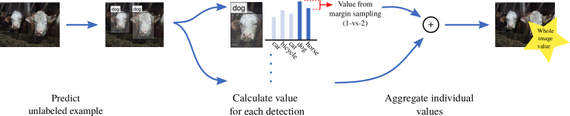
Figure 1: Pipeline for determining active learning value of a whole unlabeled image in object detection. First, bounding boxes are predicted using a method such as YOLO. For each bounding box we calculate an individual active learning value, e.g. 1-vs-2, based on the distribution of predicted classes. These values are then aggregated in order to identify valuable unlabeled images. Figure from Brust18_ALO . Note: cows are unknown at this stage in learning.

1 Introduction

Deep convolutional networks (CNNs) show impressive performance in a variety of applications. Even in the challenging task of object detection, they serve as excellent models Girshick2013RCNN ; Liu2015SSD ; Long2014FCN ; Redmon2015YOLO ; Redmon2016YOLOv2 . Traditionally, most research in the area of object detection builds on models trained once on reliable labeled data for a predefined application. However, in many application scenarios, new data becomes available over time or the distribution underlying the problem changes. When this happens, models are usually retrained from scratch or have to be refined via either fine-tuning hoffman2014lsda ; Long2014FCN or incremental learning li2016learning ; rebuffi2016icarl . In any case, a human expert has to assign labels to identify objects and corresponding classes for every unlabeled example. When domain knowledge is necessary to assign reliable labels, this is the limiting factor in terms of effort or costs. For example, cancer experts have to manually annotate hundreds of images to provide accurately labeled data qaiser2017her2 ; Rodner17_DBF .

Changing distributions can also pose a problem because constant relabeling is required. Self-driving cars for example should not be confused by new types of signage or other changes in regulation and environment. To adapt to them, additional labels need to be supplied.

In the field of biodiversity, there is a strong demand for reliable and cost-effective methods of estimating diversity indicators such as animal abundance and site occupancy mackenzie2004occupancy . Manual observation in the field can be replaced by automated camera traps. However, images from these cameras require expert analysis to be useful in biodiversity studies. Machine learning can reduce the amount of expert work required by generalizing from labeled images. Still, when new species are observed or environmental changes occur, new labels may be necessary for stable recognition performance.

The goal of active learning is to minimize this labeling effort by selecting only valuable unlabeled examples for annotation by the human domain expert. Active learning is widely studied in classification tasks, where different measures of uncertainty are the most common choice for selection ertekin2007learning ; fu2015batch ; hoi2006large ; Jain09:ALL ; Kapoor10:GP ; Kaeding2016WALI ; tong2001support .

1.1 Structure

This work is split in two parts: The first part starts by describing the tasks tackled and the active learning problem in general (see section 3). We propose two active learning methods in section 4. The first method is uniquely generic and can be applied to any object detection system unlike most related methods. The second is geared towards one of the most famous deep object detectors: “You Only Look Once” – YOLO Redmon2015YOLO . We add an incremental learning scheme Kaeding2016FDN to build an object detection system suitable for active and continuous exploration applications. We first show the validity and performance of our system in an experiment on a popular benchmark dataset in section 5. It is then applied and evaluated in a real-life situation in section 6, helping biodiversity researchers with their analysis of wildlife camera footage. The software is described in detail in section 7 and available upon request.

In the second part, section 8 gives an outlook into a more theoretically sound active learning method called Expected Model Output Change (EMOC, Freytag2014EMOC ). As a first step towards using it in our application, we validate its performance in a related scenario where object proposals from an unsupervised method are classified.

2 Related Work

2.1 Object Detection using CNNs

An important contribution to object detection based on deep learning is R-CNN Girshick2013RCNN . It delivers a considerable improvement over previously published sliding window-based approaches. R-CNN employs selective search uijlings2013selective , an unsupervised method to generate region proposals. A pre-trained CNN performs feature extraction. Linear SVMs (one per class) are used to score the extracted features and a threshold is applied to filter the large number of proposed regions. Fast R-CNN Girshick2015FastRCNN and Faster R-CNN Ren2015FasterRCNN offer further improvements.

Object detection can also be performed in a single step, combining localization and classification. An example of this is YOLO Redmon2015YOLO , short for “You Only Look Once”. The authors train a CNN end-to-end as opposed to using it simply for feature extraction. After the single pass prediction, some post-processing is required to turn the model’s representation into a list of bounding boxes. This includes thresholding and non-maximum suppression. Because YOLO can classify and localize independently, it can localize objects of unknown classes robustly. This property is important for active exploration scenarios where new classes may appear at any time.

A similar approach to YOLO is SSD Liu2015SSD . It also delivers the detections using a complex output encoding. A number of improvements make it more accurate and faster than YOLO at the same time. One improvement is the incorporation of prior knowledge about the distribution of bounding box aspect ratios. SSD also considers multiple scales during prediction.

In lin2017focal , a new loss function for single-pass object detectors is proposed to counter the effects of imbalanced positive and negative examples which are typical for detection tasks. The authors also propose an efficient implementation called RetinaNet which combines the accuracy of two-stage approaches with the speed of single-stage approaches.

YOLOv2 Redmon2016YOLOv2 improves upon the original YOLO by including aspect ratio priors for bounding boxes and more fine-grained feature maps using pass-through layers to increase resolution. The network is trained on multiple scales by resizing during training. The input size can be changed arbitrarily since it only contains convolutional and pooling layers Long2014FCN . Further small improvements are proposed in redmon2018yolov3 as YOLOv3, such as training at more scales and using a more accurate and efficient feature extraction network. We use YOLO in favor of YOLOv2/v3, RetinaNet or SSD because of its relative simplicity w.r.t. its output encoding.

2.2 Active Learning for Object Detection

The authors of abramson2006active propose an active learning system for pedestrian detection in videos taken by a camera mounted on the front of a moving car. Their detection method is based on AdaBoost while sampling of unlabeled instances is realized by hand-tuned thresholding of detections. Object detection using generalized Hough transform in combination with randomized decision trees, called Hough forests, is presented in yao2012interactive . Here, costs are estimated for annotations, and instances with highest costs are selected for labeling. This follows the intuition that those examples are most likely to be difficult and therefore considered most valuable. An active learning approach for satellite images using sliding windows in combination with an SVM classifier and margin sampling is proposed in bietti2012active . The combination of active learning for object detection with crowd sourcing is presented in vijayanarasimhan2014large . A part-based detector for SVM classifiers in combination with hashing is proposed for use in large-scale settings. Active learning is realized by selecting the most uncertain instances for labeling. In roy2016active , object detection is interpreted as a structured prediction problem using a version space approach in the so called “difference of features” space. The authors propose different margin sampling approaches estimating the future margin of an SVM classifier.

Like our proposed approach, most related methods presented above rely on uncertainty information like least confidence or 1-vs-2. However, they are designed for a specific type of object detection and therefore can not be applied directly to the output of YOLO. Additionally, our method does not propose single objects to the human annotator. It presents whole images and takes labels for every object in the image as input. We also attempt to exploit information specific to YOLO in a secondary approach and compare it to our proposed generic methods.

2.3 Active Learning for Deep Architectures

In wang2014new and Wang2016CEAL , uncertainty-based active learning criteria for deep models are proposed. The authors offer several metrics to estimate model uncertainty, including least confidence, margin or entropy sampling. Wang et al. additionally describe a self-taught learning scheme, where the model’s prediction is used as a label for further training if uncertainty is below a threshold. Another type of margin sampling is presented in stark2015captcha . The authors propose querying examples according to the quotient of the highest and second-highest class probability.

The visual detection of defects using a ResNet is presented in feng2017dal . The authors propose two methods: uncertainty sampling (i.e. defect probability of 0.5) and positive sampling (i.e. selecting every positive example since they are very rare) for querying unlabeled instances as model update after labeling. Another work which presents uncertainty sampling is liu2017active . In addition, a query by committee strategy as well as active learning involving weighted incremental dictionary learning for active learning are proposed.

In the work of gal2017deep , several uncertainty-related measures for active learning are proposed. Since they use Bayesian CNNs, they can make use of the probabilistic output and employ methods like variance sampling, entropy sampling or maximizing mutual information.

All of the works introduced above are tailored to active learning in classification scenarios. Most of them rely on model uncertainty, similar to our proposed selection criteria. We are evaluating object detection scenarios where we partly take advantage of the special output generated by YOLO. Thus, these works can not be applied directly.

Besides estimating the uncertainty of the model, further retraining-based approaches are maximizing the expected model change huang2016active or the expected model output change Kaeding2016AEMOC that unlabeled examples would cause after labeling. Since each bounding box inside an image has to be evaluated according its active learning value, both measures would be impractical in terms of runtime without further modifications. First steps towards using EMOC for detection are outlined in section 8.

A more complete overview of general active learning strategies can be found in Grauman2016Crowd ; Settles2009ALS .

2.4 Human-Computer Interaction

While efficient sampling of unlabeled data for later annotation is an important step towards better use of expert time and funding, there are other aspects of a learning system that have potential for improvement, namely the human-computer interaction. Weak supervision in general is the use of labels or supervision signals that are less precise, accurate or complex than actually required by the task at hand Zhou2017 . This usually means that more labels are needed to reach a certain accuracy. However, interaction times can be faster, leading to a net gain for certain weakly supervised methods. Less precise labels may also be more widely available or cheaper.

In Papdopoulos2016Semi , the authors propose an interaction scheme for annotating bounding boxes. Proposals for bounding boxes are generated and the annotator can only verify, or in certain setups, modify them. This reduces the annotation time substantially compared to manual painting of bounding boxes, but also leads to verification of bounding boxes that are not perfect. In their experiments, they show that the trade-off works in favor of their proposed method, the concept of which we also adopt in our system (see sections 6 and 7).

Extreme clicking papadopoulos2017extreme is an approach which requires manual annotation, but in a more reasonable manner. Instead of requesting the often non-existent top left and bottom right corners of an object, the user selects four extreme points in the top, bottom, left, and right directions. This leads to a 5x speedup in interactions without any loss of accuracy.

2.5 Automated Wildlife Surveillance

The work gomez2016animal presents a study of the effectiveness of different deep learning architectures on deciding first if an image shows a bird or mammal and deciding the correct mammal set afterwards using the Snapshot Serengeti dataset swanson2015snapshot . Forwarding images with low confidence decisions to a human expert allows for reaching high accuracies.

A related approach is proposed in norouzzadeh2017automatically where animals are classified after deciding if an image contains an animal at all. This work presents a study of different CNN architectures also using the Snapshot Serengeti dataset. Another study with a deeper evaluation on different subsets of this dataset involving species-level accuracies was presented in gomez2017towards .

Animal segmentation using Multi-Layer Robust Principal Component Analysis involving color and texture features was proposed in giraldo2017camera . This approach was further combined with deep learning methods in giraldo2017automatic . Both works are evaluated on camera trap data from a Colombian forest.

In contrast to those approaches, we do not rely on a fixed training set but explicitly acquire new training data to improve our model. Additionally, we are able to handle images showing more than one animal since we use detection methods instead of assigning whole image labels.

An animal re-identification approach based on object proposals, which are then used to extract faces for classification, is presented in Brust_2017_ICCV . This method also relies on YOLO to generate class-independent proposals.

3 Background: Classification, Detection, Supervision and the Active Learning Problem

This section serves to introduce the notation used and problems tackled throughout the first part of this work.

Classification

is a machine learning task in which an example $x$, e.g. an image or text, from a data space $\mathfrak{D}$ is assigned a class $c$ from a set $C$ of many possible classes, e.g. cat or dog. For our purposes, we require a classifier to not only assign a class $c$, but predict a distribution over all classes $C$ given an example $x$. As such, we define a classifier function $f_{c}$ (also called score) per class $c\in C$:

$$f_{c}:x\mapsto\hat{p}(c|x)\enspace\text{with }\sum_{c\in C}f_{c}(x)=1\enspace.$$ (1)

In the following sections, we will mostly look at the classifier output in the form of the estimated distribution $\hat{p}$.

Detection

or object detection is a more complex task where a non-fixed number of instances of classes in an image $x$ is both localized and classified. For a given image $x$, a detector produces $D$ different detections depending on the content of $x$. For each detection (indexed $i$), a bounding box $B_{i}=(x,y,w,h)_{i}$ and class distribution $\hat{p}_{i}(c,x)$ are estimated:

$$f_{c,i}:x\mapsto(B_{i},\hat{p}_{i}(c|x))\enspace\text{with }\sum_{c\in C}f_{c,i}(x)=1\enspace.$$ (2)

The following sections will focus on the estimated distributions $\hat{p}_{i}$ of a detector.

3.1 Incremental Learning

Typically, classifiers and detectors are trained once, “seeing” all training data, and then used indefinitely without any further adjustments. For long-running applications, this setup can become problematic: over time, a problem domain can change or extend, e.g. to new classes. Instead of time- and resource-intensive retraining, one can also apply incremental learning. Here, an existing model is augmented such that it learns any new training data without “forgetting” about the previous observations.

3.2 Weakly Supervised Learning

In most cases, classifiers and detectors are trained in a supervised fashion, meaning that the training data is made up of pairs of examples and labels $(x,y)$. In contrast, unsupervised learning considers only the examples themselves, without labels. Examples include clustering methods as well as generative models. Weakly supervised learning is a compromise: labels are available, but are of reduced quality or information content. This technique can be used to trade-off annotation time against label quality in an effort to achieve better accuracy within a given amount of annotation time.

3.3 Active Learning

Active learning is the problem of selecting examples $x$ from an unlabeled pool $\mathfrak{U}$ for labeling, e.g. by a human annotator, such that the performance of a future machine learning task is maximized when the selected and annotated examples are learned. The ultimate goal is to increase data efficiency and to minimize the need for manual annotation. The active learning problem can be rephrased as a value assignment, where higher values indicate better future performance when the example is labeled and used for training. Each example $x$ is assigned a value in $[0,1]$ by a function $v(x)$, also called an active learning metric. Selection is then performed by sorting all candidate unlabeled examples by their value and choosing the desired amount of top examples.

Active learning is often used in conjunction with incremental learning of small batches. Many active learning methods incorporate the prediction of an existing model into their value function, which might change substantially after learning only a few examples. As such, a tight feedback loop is important for good data efficiency.

The predictions of a model on unseen, unlabeled examples, can be analyzed for uncertainty. Uncertainty is one of the most common concepts in active learning ertekin2007learning ; fu2015batch ; hoi2006large ; Jain09:ALL ; Kapoor10:GP ; Kaeding2016WALI ; tong2001support , as it serves as a reasonable indicator of valuable examples.

1-vs-2

An estimated distribution $\hat{p}(c|x)$ can be analyzed for indications of uncertainty. For example, if the difference between the two highest class probabilities is very low, the example may be located close to a decision boundary. In this case, it can be used to refine the decision boundary and is therefore valuable. Its value is determined using the highest scoring classes $c_{1}$ and $c_{2}$, and the following definition:

$$v_{1vs2}(x)~{}=~{}1-(\underset{c_{1}\in C}{\textrm{max}}\,\hat{p}(c_{1}|x)-\underset{c_{2}\in C\setminus c_{1}}{\textrm{max}}\,\hat{p}(c_{2}|x))\enspace.$$ (3)

This metric is known as 1-vs-2 or margin sampling Settles2009ALS . We use 1-vs-2 as part of our methods since its operation is intuitive and it can produce better estimates than e.g. least confidence approaches Kaeding2016AEMOC . A possible alternative is outlined in section 8.

4 Our Methods: Active Learning for Deep Object Detection

The active learning problem can also be posed for detection tasks. We consider the value of labeling whole images $x$ even for detection, as opposed to individual objects or regions.

In this section, we propose two approaches. First, a method to adapt any distribution-based active learning metric for classification to object detection using an aggregation process. This method is applicable to any object detector whose output contains class scores for each detected object. Second, two metrics specific to the YOLO Redmon2015YOLO object detector are described, using implementation-specific information not available to all object detectors.

4.1 Aggregated Detection Metrics

Using a classification metric on a single detection is straightforward, if class probabilities are available. However, aggregating metrics for a complete image can be done in many different ways. Possible aggregations include calculating the sum, the average or the maximum over all detection values. However, for some aggregations, it is not clear how an image without any detections should be handled.

Sum

A straightforward method of aggregation is the sum. Intuitively, this method prefers images with lots of uncertain detections in them. When aggregating detections using a sum, empty examples should be valued zero. It is the neutral element of addition, making it a reasonable value for an empty sum. A low valuation effectively delays the selection of empty examples until there are either no better examples left or the model has improved enough to actually produce detections on them. It should be noted that the range of this function is not necessarily $[0,1]$. The value of a single example $x$ can be calculated from the detections $D$ in the following way, where $v_{1vs2}(x_{i})$ denotes an application of $v_{1vs2}$ w.r.t. $\hat{p}_{i}$:

$$v_{Sum}(x)~{}=~{}\sum_{i\in D}v_{1vs2}(x_{i})\enspace.$$

Average

Another possibility is averaging all detection values. The average is not sensitive to the number of detections, which may make values more comparable between images. If an example does not contain any detections, it will be assigned a zero values. This is an arbitrary rule because there is no true neutral element w.r.t. averages. However, we choose zero to keep the behavior in line with the other metrics:

$$v_{Avg}(x)~{}=~{}\frac{1}{|D|}\sum_{i\in D}v_{1vs2}(x_{i})\enspace.$$

Maximum

Finally, individual detection values can be aggregated by calculating the maximum. This can result in a substantial information loss. However, it may also prove beneficial because of increased robustness to noise from many detections. For the maximum aggregation, a zero value for empty examples is valid. The maximum is not affected by zero valued detections, because no single detection’s value can be lower than zero:

$$v_{Max}(x)~{}=~{}\underset{i\in D}{\textrm{max}}\enspace v_{1vs2}(x_{i})\enspace.$$

4.2 YOLO Specific Metrics

YOLO Redmon2015YOLO offers an end-to-end approach to deep learning-based object detection. Both its high recognition rate and its real-time property are a result of the compact output encoding. A fixed size vector stores (within certain boundaries) an arbitrary amount of detections. To achieve this, the image is divided into $S_{h}\cdot S_{v}$ equally sized grid cells. For each cell $i$, class scores $\hat{p}_{i}(c)$ are predicted. Furthermore, the model predicts $B$ bounding boxes, including coordinates relative to the cell’s center, dimensions and an estimated confidence value $\hat{C}$ to describe a region’s “objectness”. Adapting classification metrics to object detection can be done by evaluating single detections and aggregating the results for a complete example (fig. 1). However, the YOLO detector’s output contains information beyond the detections themselves. Specifically, it predicts a detection confidence $\hat{C}$ between 0 and 1 separately from the classification scores.

When incorporating the model’s detection confidence into a metric, the following detection-specific scenarios can be reacted to: (i) An image cell has a very high class score, indicating a confident classification, but low predicted detection confidence. This situation can be caused by a missed detection of a known object class. (ii) A cell has very low class scores overall, but a high confidence estimate. This may indicate an unknown object class.

Note that because of the way YOLO is implemented and the metrics are designed, the values $v(x)$ are not bound to be in the range $[0,1]$.

Detection-Classification Difference

Either scenario can be considered a valuable example because it represents uncertainty in the model. We propose the Detection-Classification Difference metric. It aims to detect both scenarios by calculating the absolute difference between the predicted confidence $\hat{C}$ and the highest class score $\hat{p}$:

$$v_{DetClassDiff}(x)~{}=~{}\sum_{i=0}^{S_{h}S_{v}}\| \underset{j=1,\dots,B}{\textrm{max}}\,\hat{C}_{i,j}$$

$$-\underset{c\in C}{\textrm{max}}\,\hat{p}_{i}(c|x)\|^{2}\enspace.$$ (4)

Weighted Cell Sum

An adapted classification metric can also be enhanced by using additional information from YOLO, specifically the predicted confidence $\hat{C}$. The adapted metric is calculated individually for all cells and then aggregated as a weighted sum, using the predicted confidences $\hat{C}$ for each cell as weights. We adapt the 1-vs-2 metric similar to the methods from section 4.1, resulting in the Weighted Cell Sum metric:

$$v_{WCellSum}(x)~{}=~{}\sum_{i=0}^{S_{h}S_{v}}\| \underset{j=1,\dots,B}{\textrm{max}}\,\hat{C}_{i,j}$$

$$\cdot v_{1vs2}(x_{i})\|^{2}\enspace.$$ (5)

Assuming high confidence estimates $\hat{C}$ (i.e. non-objects close to zero and detections close to one), this metric is very similar to the proposed Sum aggregation that operates only on the detections. With perfect confidence values, the only differences would be the result of post-processing, e.g. non-maximum suppression Redmon2015YOLO , which is rarely necessary.

Note that the average or maximum operations are not applicable here. A weighted average would produce identical results to the sum as the number of “detections”, or grid cells, is constant. A maximum could either ignore the weights, which would likely result in a constant high value, or take them into account, in which case it approximates the Max variant from the previous section.

Algorithm 1: Detailed description of the experimental protocol. Please note that in an actual continuous learning scenario, new examples are always added to $\mathfrak{U}$. The loop is never left because $\mathfrak{U}$ is never exhausted. The described splitting process would have to be applied regularly.

Known labeled examples $\mathfrak{L}$, unknown examples $\mathfrak{U}$, initial model $f_{0}$, active learning metric $v$

$\mathfrak{U}=\mathfrak{U}_{1},\mathfrak{U}_{2},\ldots\leftarrow$ split of $\mathfrak{U}$ into random batches

$f\leftarrow f_{0}$

while $\mathfrak{U}$ is not empty do

    calculate predictions for all unlabeled batches in $\mathfrak{U}$ using $f$

    $\mathfrak{U}_{best}\leftarrow$ highest scoring unlabeled batch in $\mathfrak{U}$ according to $v$

    

    $\mathcal{Y}_{best}\leftarrow$ annotations for $\mathfrak{U}_{best}$ human-machine interaction

    $f\leftarrow$ incrementally train $f$ using $\mathfrak{L}$ and update batch $(\mathfrak{U}_{best},\mathcal{Y}_{best})$

    

    $\mathfrak{U}\leftarrow\mathfrak{U}\backslash\mathfrak{U}_{best}$

    $\mathfrak{L}\leftarrow\mathfrak{L}\cup(\mathfrak{U}_{best},\mathcal{Y}_{best})$

end while

5 Experiment: PASCAL VOC 2012

	50 Samples	100 Samples	150 Samples	200 Samples	250 Samples	All Samples
	mAP / AUC	mAP / AUC	mAP / AUC	mAP / AUC	mAP / AUC	mAP / AUC
Baseline
Random	$8.7$/$4.3$	$12.4$/$14.9$	$15.5$/$28.8$	$18.7$/$45.9$	$21.9$/$66.2$	$32.4$/$264.0$
Our Methods (YOLO Specific)
Det.-Class. Diff.	$8.5$/$4.3$	$12.1$/$14.6$	$15.5$/$28.4$	$18.7$/$45.5$	$21.0$/$65.3$	$\bf 33.3$/$255.3$
Weighted Cell Sum	$\bf 9.6$/$\bf 4.8$	$12.9$/$\bf 16.1$	$16.6$/$30.8$	$\bf 20.5$/$49.4$	$21.9$/$70.6$	$32.2$/$268.1$
Our Methods
Max	$9.2$/$4.6$	$12.9$/$15.7$	$15.7$/$30.0$	$19.8$/$47.8$	$22.6$/$69.0$	$32.0$/$\bf 269.3$
Avg	$9.0$/$4.5$	$12.4$/$15.2$	$15.8$/$29.2$	$19.3$/$46.8$	$\bf 22.7$/$67.8$	$33.3$/$266.4$
Sum	$8.5$/$4.2$	$\bf 14.3$/$15.6$	$\bf 17.3$/$\bf 31.4$	$19.8$/$\bf 49.9$	$22.7$/$\bf 71.2$	$32.4$/$268.2$

Table 1: Validation results on part B of the PASCAL VOC 2012 dataset, i.e. new classes only. Bold indicates best results.

Our goal is to design an application suitable for automated wildlife surveillance based on camera trap image analysis involving minimal human supervision while ongoing streams of unlabeled input data occur. However, we cannot evaluate all methods on the camera trap data because of the limited availability of labels. Therefore, use the PASCAL VOC 2012 dataset Everingham2010VOC to pose two research questions: (i) can any of our proposed metrics perform better than random selection and (ii) which metric performs best.

We then use the best performer for our camera trap experiment in the next section.

Methods and Baseline

The methods compared in this experiment are those proposed in the previous section. First, the 1-vs-2 metric aggregated using Sum, Max and Avg. Second, the YOLO-specific Detection-Classification Difference and Weighted Cell Sum.

We use random selection for comparison. To the best of our knowledge, there are no competing active learning methods that value examples for object detection on an image level at this time.

Data

We use the PASCAL VOC dataset Everingham2010VOC to assess the effects of our methods on learning. To specifically measure incremental and active learning performance, both training and validation set are split into parts A and B in two different random ways to obtain more general experimental results. Part B is considered “new” and is comprised of images with specific classes depending on the split. Part A contains all other 17 classes and is used for initial training. The training set for part B contains 605 and 638 images for the first and second way, respectively.

Active Exploration Protocol

The experiment follows a typical batchwise incremental and active learning setup Kaeding2016WALI . Before an experimental run, the VOC (part B) datasets are divided randomly into unlabeled batches of 10 examples each. This fixed assignment decreases the probability of very similar images being selected for the same unlabeled batch compared to always selecting the highest valued examples, which would lead to less diverse update batches. This is valuable while dealing with data streams, e.g. from camera traps, or data with low intra-class variance. The unlabeled batch size is a trade-off between a tight feedback loop (smaller batches) and computational efficiency (larger batches).

The unlabeled batches are assigned a value using the sum of the active learning metric over all images in the corresponding unlabeled batch as a meta-aggregation. Other functions such as average or maximum could be considered, but are beyond the scope of this paper.

The highest valued unlabeled batch is selected as an update batch for an incremental training step Kaeding2016FDN . The network is updated using the annotations from the dataset in lieu of a human annotator. Annotations are not needed for update batch selection. This process is repeated from the point of unlabeled batch valuation until there are no unlabeled batches left. The assignment of examples to unlabeled batches is not changed during an experimental run, but between runs.

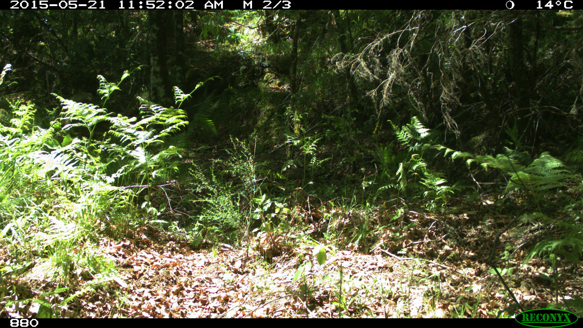
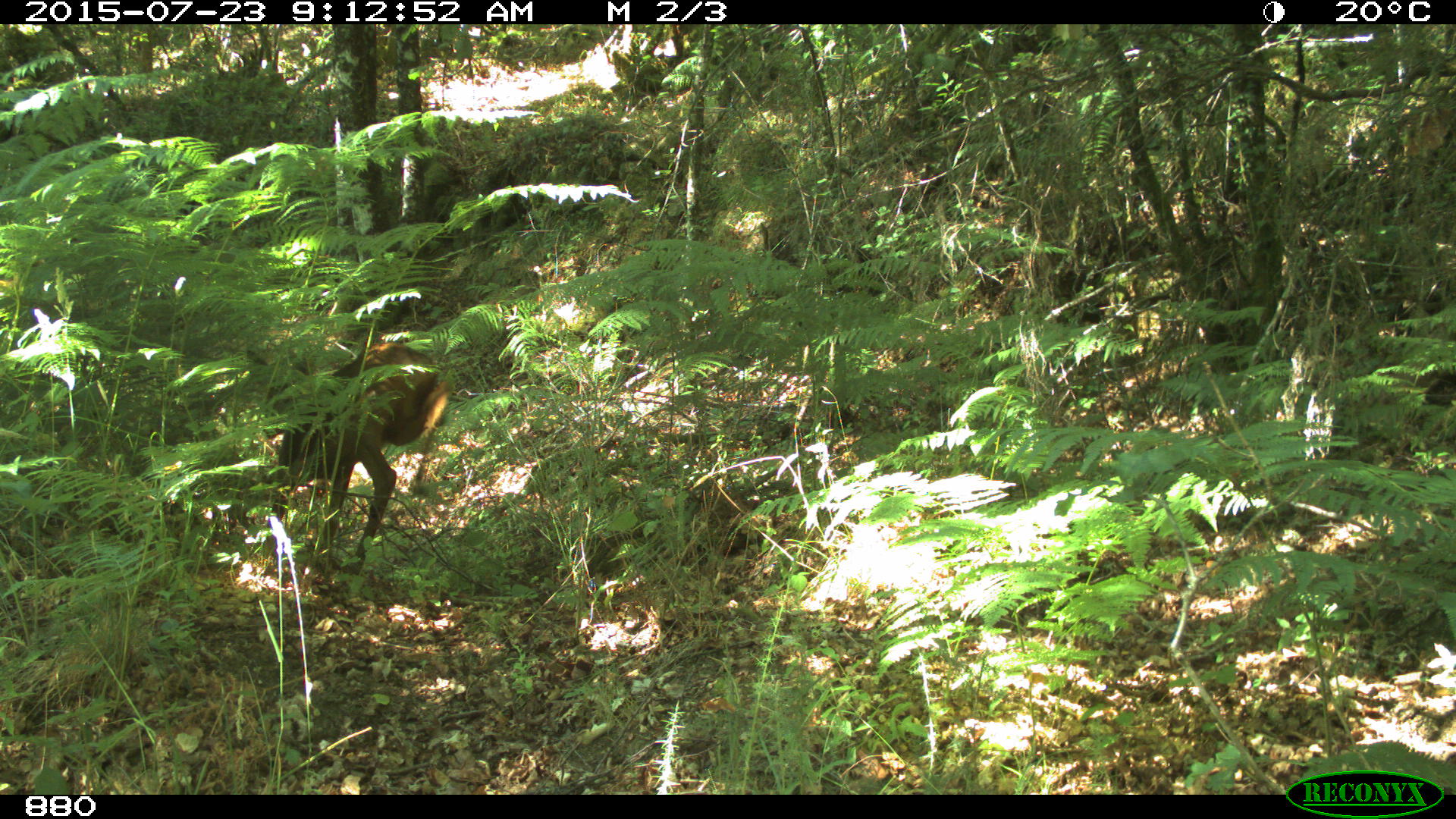
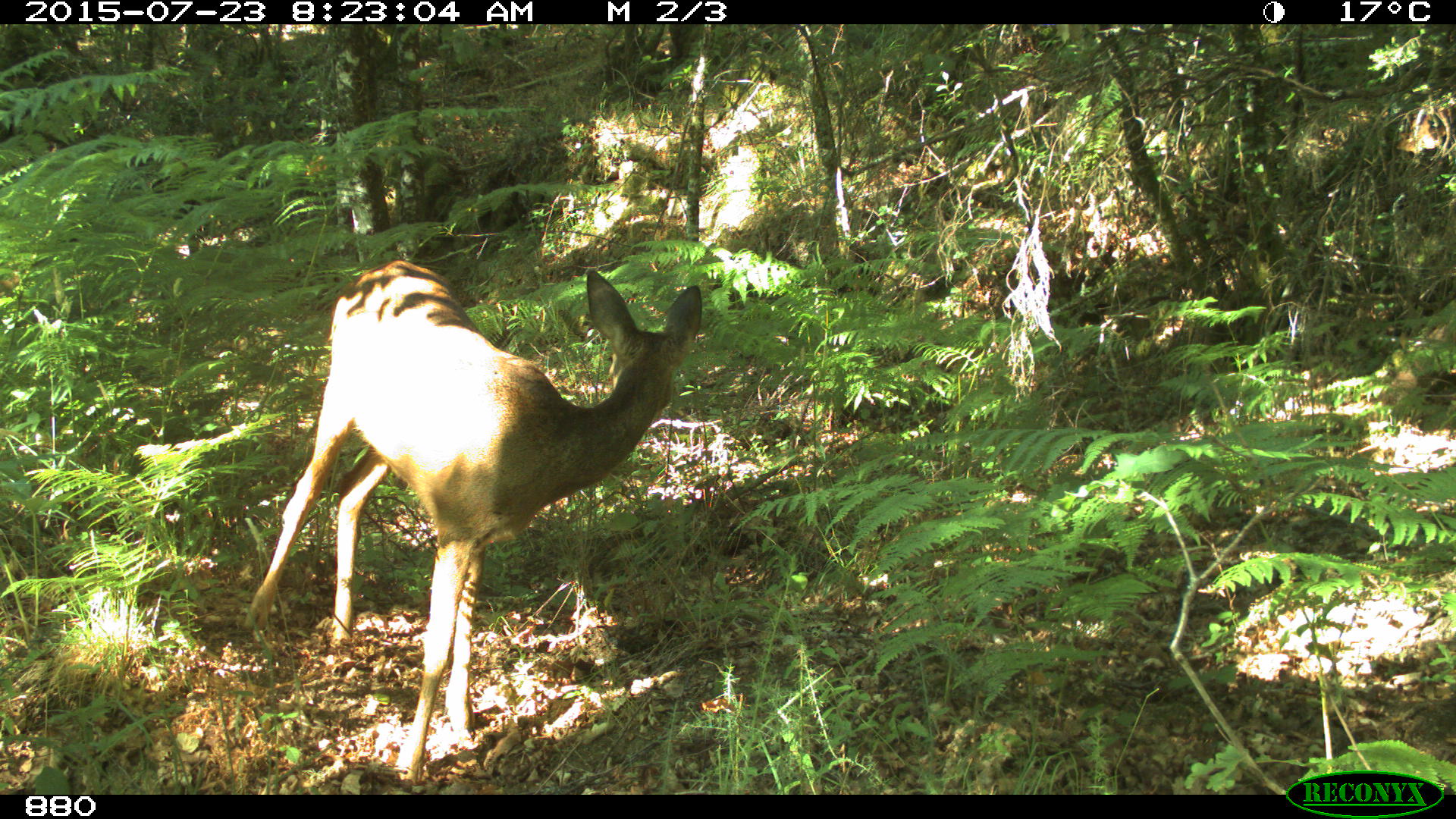
Figure 2: Camera trap images. From left to right: background only, partial occlusion, perfect visibility.

Evaluation

We report mean average precision (mAP) as described in Everingham2010VOC . For evaluation, we use measures averaged over five runs for each active learning metric as well as random selection, and each way of splitting.

We show results over the new VOC (part B) classes both in a fast exploration context (i.e. after selection of only 150 examples) and after learning all available data. Gaining accuracy as fast as possible while minimizing the human supervision is one of the main goals of active learning. Moreover, in continuous exploration scenarios, like faced in camera feeds or other continuous automatic measurements, it is assumed that new data is always available faster than can be annotated. Hence, the pool of valuable examples will rarely be exhausted.

We also report AUC, measuring mAP percent points over samples. One unit on the x axis represents 50 samples. The AUC is not normalized and can thus reach a maximum of higher than 100. It only serves to indicate stability of a method over time and is intended as a sanity check of all methods.

Setup – YOLO

We use the YOLO-Small architecture as an alternative to the larger YOLO network, because it allows for much faster training Redmon2015YOLO . Our initial model is obtained by adapting the Extraction model and training on the VOC (part A) dataset for 24,000 iterations using the Adam optimizer Kingma2014Adam . The first half of initial training is completed with a learning rate of 0.0001. The second half and all incremental experiments use a lower learning rate of 0.00001 to prevent divergence. Other hyperparameters match those used in Redmon2015YOLO , including the augmentation of training data using random crops, exposure or saturation adjustments. The implementation is done in CN24 Brust2015CPN , an open-source deep learning framework.

Setup – Incremental Learning

Extending an existing CNN without sacrificing performance on known data is not a trivial task. Fine-tuning a CNN exclusively on new data quickly leads to a severe degradation of recognition rates on previously learned examples Kirkpatrick2016Cat ; Shmelkov2017Detector .

We use our straightforward, but effective fine-tuning method Kaeding2016FDN to implement incremental learning. With each gradient step, the mini-batch is constructed by randomly selecting from old and new examples with a certain probability of $\lambda$ or $1-\lambda$, respectively. After completing the learning step, the new data is simply considered old data for the next step. Management of per-example selection probabilities is not necessary. This method can balance known and unknown data performance successfully. We use a value of 0.5 for $\lambda$ to make as few assumptions as possible and perform 100 iterations per update.

Algorithm 1 contains a detailed description of the training procedure. In our experiments, the cycle ends after all examples are labeled. In a real-world scenario, the algorithm never leaves the loop because new unlabeled examples are added continuously.

5.1 Results

The learning characteristics of each proposed method on the new classes from VOC (part B) are shown in table 1. In our case, the number of examples added equals the number of images in our experiment. Validation is performed each time after adding 50 new examples to the current model. We focus our analysis on the new, unknown data. However, not losing performance on known data is also important. The incremental learning method from Kaeding2016FDN causes only minimal losses on known data. In the worst case, the mAP on part A of the VOC dataset decreases from 36.7% to 31.9%. These losses are also referred to as “catastrophic forgetting” in literature Kirkpatrick2016Cat . The fine-tuning method does not require additional parameters or memory for added examples like comparable approaches such as Shmelkov2017Detector do. This property is an important step towards “lifelong learning”, where learning systems can run indefinitely.

Evaluation

To assess the performance of our methods in a fast exploration context, we evaluate the models after learning 150 examples. At this point there is still a large number of diverse examples for the methods to choose from, which makes the following results much more relevant for practical applications than results on the full dataset.

We see Detection-Classification Difference perform worst in fast exploration. Random selection offers comparable results with less variance. Average and Maximum perform almost equal to random selection with a very slight advantage. The best performing fast exploration method is Sum with an mAP score of 17.3%, improving the random baseline by 1.8%. Weighted Cell Sum shows similar characteristics with an improvement of 1.1%. This result falls in line with our hypothesis that both methods should show similar selection behavior because, under ideal conditions, they perform the same calculations (see section 4.2).

Surprisingly, metrics specific to YOLO do not generally perform better than the aggregation-based methods. They may be more sensitive to noise because they are calculated before YOLO’s thresholding operation. Another possible reason is non-maximum suppression. However, it is unlikely as it only affects a small number of cases Redmon2015YOLO .

All Available Examples

In our case, active learning only affects the sequence of unlabeled batches if we train until there is no new data available. Therefore, there are only very small differences between each method’s results after training has completed. However, in continuous exploration, it is usually assumed that there will be more new unlabeled data available than can be processed. Nevertheless, evaluating the long term performance of our metrics is important to detect possible deterioration over time compared to random selection. Detection-Classification Difference achieves the best results by a very small margin when querying all possible training examples. These small differences also indicate that the chosen incremental learning technique is suitable for the faced scenario.

Discussion

From the results, we conclude two points: (i) random selection can be outperformed by some of our active learning metrics, and (ii) the Sum aggregated detection metric performs best. After this result, we use the Sum metric in the following section.

6 Experiment: Camera Trap Image Analysis

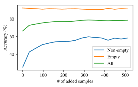
Figure 3: Camera trap image results from validation set.

After validating the correct operation of our incremental and active learning system on the PASCAL VOC benchmark dataset, we apply it to camera trap image analysis in the field of biodiversity. This is to answer an important question: can the proposed method be applied successfully in real-life scenarios? For this application, we implement a weakly supervised system where users are asked to label images selected using our proposed Sum metric, which performed best in the previous experiment’s fast exploration scenario. It tends to favor images with many proposed bounding boxes in it. Labels are acquired in a propose-and-confirm fashion to increase efficiency Papdopoulos2016Semi . The system is described in detail in section 7. The target application is represented by a large biodiversity dataset created in the course of a project at the German Centre for Integrative Biodiversity Research (iDiv) studying the impact of large herbivorous mammals on forest development in the National Park of Peneda-Gerês in Northern Portugal. Up to 65 cameras were deployed in an area of $\sim$16 km² for a period of 3-4 months in the years 2015 and 2016, resulting in a dataset of around 1.5 million images. The cameras captured around 15 species of mammals.

Figure 2 shows a variety of conditions present in the dataset. Animals are often occluded by vegetation, camouflaged on purpose to avoid predators or captured from a large distance. Further difficulties include motion blur, large herds of animals, time of day, as well as unintentional triggers of the camera trap by humans or moving leaves.

6.1 Evaluation

After validating our method on PASCAL VOC in the previous chapter, we now test it on a separately annotated part of the dataset consisting of 5,000 examples with image level class labels only. For labeling and training, there are another 5,000 images to select from.

To evaluate the detector in spite of missing bounding box annotations, its output is interpreted as a multi-label classifier output. All other parameters match those detailed in section 5. By mapping the classes of the PASCAL VOC dataset Everingham2010VOC to the observed species, the initial model achieves an accuracy of 66.5%. After labeling 512 of the 5,000 training images selected by the Sum method using experts in a fast exploration-like scenario, the accuracy increases to 78.7%.

Only 37.8% of images in the dataset contain objects. Figure 3 shows results on empty and non-empty images separately. On the non-empty subset, accuracy increases from 25.4% to 42.6% after labeling only 32 examples, reaching a final value of 58.5%.

Longer-term usage could improve the model even further. Weakly supervised learning on average requires more labels than fully supervised learning to achieve the same performance. However, it has an overall advantage due to much shorter labeling times per image Papdopoulos2016Semi .

From this experiment, we conclude that our combination of active and incremental learning can be applied successfully to a real-life camera trap image analysis scenario.

7 Software: Carpe Diem Annotation Tool

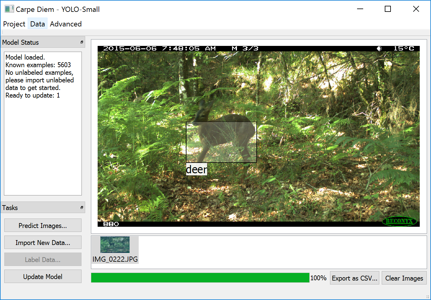
Figure 4: Carpe Diem main screen.

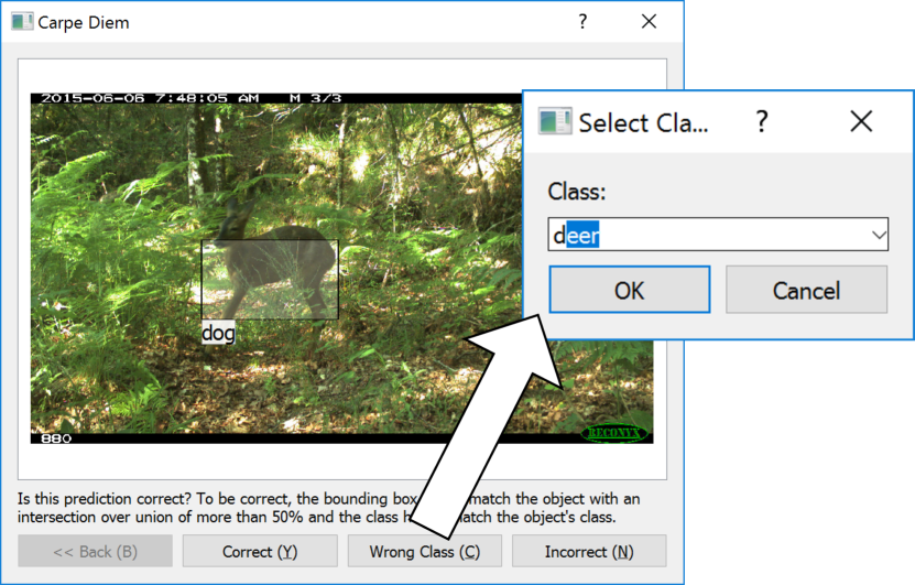
Figure 5: Carpe Diem annotation screen.

In this section, we briefly describe the implementation of our annotation tool offered to biodiversity experts. This tool, called Carpe Diem, realizes a learning cycle environment in a graphical user interface (see fig. 4). A learning cycle consists of selection (active learning), label acquisition (user interaction) and model update (incremental learning) and is executed repeatedly, as new labeling resources become available. YOLO Redmon2015YOLO is used as a detection model and for generating proposals. It is implemented using the CN24 Brust2015CPN framework.

Carpe Diem’s clean and simple interface offers all necessary choices and is intuitive to use, even for inexperienced users. The user can first load or create an annotation project. This collects labeled and unlabeled data as well as a model in one place. When a project is loaded, the user can generate predictions for images and visualize or export them. Additional labeled and unlabeled data can be loaded. If there is labeled data that has not yet been observed by the model, a training button is available.

The main purpose of Carpe Diem lies in the labeling. When the user wishes to label data, a press of a button starts the evaluation of all unlabeled data against the criteria described in section 4. The highest scoring batch is then presented for labeling in a weakly supervised fashion as described in section 6.

The interaction is designed as follows. For each proposed bounding box, the annotator can choose to either confirm it, reject it entirely, or assign a different class (see fig. 5). If a reassigned class is unknown, the model will be adapted automatically. After labeling the batch, the user simply clicks the training button to update the model. The training function takes into account the number of newly labeled images and uses our incremental learning method presented in Kaeding2016FDN .

Carpe Diem is available to researchers on request.

8 Outlook: Expected Model Output Change

The ultimate goal of active learning is to reduce the risk of models after new examples have been added. Trying to achieve this in practice reveals substantial problems such as the absence of the labels necessary to obtain the future risk or the usually small portion of labeled data making it hard to give reliable estimates for the risk (see Kaeding15_ALD for a more detailed introduction on this).

To tackle these problems, the use of surrogates as selection criterion (such as relying on the classification or detection scores like in our methods proposed above) is common practice. These surrogates show remarkable results in actual applications, such as our wildlife monitoring scenario. However, researchers also developed approaches using approximations leveraging the search for the smallest future risk. Some examples for this are li2014multi ; roy2001toward ; Settles2009ALS ; vijayanarasimhan2011cost ; wang2010discriminative . In the following, we will briefly review the expected model output change (EMOC) criterion which is indeed an upper bound for the reduction of future risk (a detailed proof is given in Freytag2014EMOC ; Kaeding15_ALD ). While this approach was already transferred to deep neural networks in Kaeding2016ACE , we will demonstrate the performance of the method on an unsupervised detection task using object proposals using Gaussian processes (GP).

This setting is closely related to our application presented in the previous sections. As is, it is not directly applicable to our deep detection scenario, but could be extended to the application in the future. This section should thus serve as a self-contained outlook into more theoretically sound methods of active learning, and the experiments as a first step towards this goal.

Additionally, we will introduce how the EMOC criterion can be extended to handle unnameable instances. These are queries that cannot be answered by the annotator, possibly because of lack of expertise. In our wildlife monitoring application, such cases are to be expected and should be handled properly.

8.1 Definition of EMOC

As introduced, the estimation of risk reduction incurred by a newly labeled example has to deal with severe problems. To leverage this, Freytag2014EMOC ; Kaeding15_ALD proposes to favor the selection of unlabeled examples that are most likely to change the model output into any direction. While this can be traced back to maximizing an upper bound on error reduction from a theoretical perspective, a more intuitive interpretation would be to search for information that “shake the view on the world” of the current model. The resulting EMOC criterion can be formalized as follows:

$$\Delta f(\mathbf{\boldsymbol{x}}^{\prime}) =\mathbb{E}_{c^{\prime}\in C}\;\mathbb{E}_{\mathbf{\boldsymbol{x}}\in\mathfrak{D}}\left(\mathcal{L}\left(f(\mathbf{\boldsymbol{x}}),f^{\prime}(\mathbf{\boldsymbol{x}})\right)\right)\enspace.$$ (6)

Here, $f(\cdot)$ stands for the current model while $f^{\prime}(\cdot)$ is the future model updated with the new example $(\mathbf{\boldsymbol{x}}^{\prime},c^{\prime})$. Since the label $c^{\prime}$ is unknown, the final values is marginalized over every possible known class in the label space $C$. We also experimented with explicitly incorporating the possibility of new classes, but found no superior behavior given a more complex estimate. Furthermore, the change is estimated over the whole available input space $\mathfrak{D}$ which includes known as well as unlabeled examples. This general formulation still requires to be implemented. Hence, we will shed some light on a suitable realization in the following.

Choice of the Model Function

In the following we will rely on GPs which allow for closed form model updates, i.e. the step from $f(\cdot)$ to $f^{\prime}(\cdot)$ (see Freytag13_LET ). This is beneficial for two reasons. First, the EMOC criterion can be reformalized which allows for a much more efficient computation. Second, the actual update after an example is selected and annotated can be done much faster. Furthermore, choosing GPs as underlying model family allows for further approximations and application scenarios (see e.g. Kaeding2016AEMOC ; Kaeding18_ALR ).

Choice of the Loss Function

In Freytag2014EMOC , the choice of the absolute difference of the model outputs was suggested as a suitable loss function. Since we use the one-vs-all technique, we learn $C$ binary classifiers $f_{c}$ with GP regression when a classification problem with $C$ classes is given. Each of the classifiers gives a continuous classification score $f_{c}(\mathbf{\boldsymbol{x}})\in\mathbb{R}$, which is used to perform classification decisions according to:

$$\bar{y}(\mathbf{\boldsymbol{x}}) =\underset{c=1\ldots C}{\operatorname{argmax}}\;f_{c}(\mathbf{\boldsymbol{x}})\enspace.$$ (7)

Combining both aspects leads to the following formalization:

$$\mathcal{L}_{1}\left(f\left(\mathbf{\boldsymbol{x}}\right),f^{\prime}\left(\mathbf{\boldsymbol{x}}\right)\right)) =\sum\limits_{c=1}^{C}|f_{c}(\mathbf{\boldsymbol{x}})-f_{c}^{\prime}(\mathbf{\boldsymbol{x}})|\enspace.$$ (8)

While the loss can in general be chosen arbitrarily, we stick to the $\mathcal{L}_{1}$ loss for the shown experiments. Please see Kaeding15_ALD for an evaluation considering more options.

Choice of Multi-class Classification Probabilities

We compute multi-class probabilities directly derived from uncertainty estimates Froehlich13:GSS . The underlying idea of the uncertainty technique is that for label regression with GPs, we do not only have the model prediction $f_{c}(\mathbf{\boldsymbol{x}})$ but rather the whole posterior distribution $\mathcal{N}(f_{c}(\mathbf{\boldsymbol{x}}),\sigma^{2}(\mathbf{\boldsymbol{x}}))$ independently for each binary classification problem involved in the one-vs-all problem. The probability of class $c$ achieving the maximum score in EQ. (7) can therefore be expressed by:

$$p\!\left(\bar{y}(\mathbf{\boldsymbol{x}})=c|\mathbf{\boldsymbol{x}}\right) =p\!\left(c=\underset{c^{\prime}=1\ldots C}{\operatorname{argmax}}\;f_{c^{\prime}}(\mathbf{\boldsymbol{x}})\right)\enspace.$$ (9)

To estimate the probabilities, we apply a Monte-Carlo technique and sample $Z$ times from all $C$ Gaussian distributions $\mathcal{N}(f_{c}(\mathbf{\boldsymbol{x}}),\sigma^{2}(\mathbf{\boldsymbol{x}}))$ and estimate the probability of each class:

$$p\!\left(y=c|\mathbf{\boldsymbol{x}}\right)=p\!\left(\bar{y}(\mathbf{\boldsymbol{x}})=c|\mathbf{\boldsymbol{x}}\right) \approx\frac{Z_{c}}{Z}\enspace,$$ (10)

with $Z_{c}$ denoting the number of times where the draw from the distribution of class $c$ was the maximum value. A large variance $\sigma^{2}$, i.e. a high uncertainty of the estimate, leads to a nearly uniform distribution $p\!\left(y=c\right)$, whereas a zero variance results in a distribution which is equal to one for the class which corresponds to the highest posterior mean. An evaluation considering more options is given in Kaeding15_ALD .

8.2 Active Learning with Unnameable Instances

A very common assumption in active learning is that the oracle (e.g. a human annotator) can provide a label for every instance of the set of unlabeled examples. Especially for tasks that involve a large set of categories, this assumption is not reasonable. There may be further complications due to occlusions, which are a large problem in wildlife monitoring and can make it impossible to assign a label. Therefore, we have to deal with cases where the oracle rejects to label the example that the active learning algorithm just selected. From our experience, there are basically two main scenarios in which a rejection can possibly happen. Both cases need to be considered during active learning and we present solutions and adaptations of the EMOC principle for each of them in the following.

Dealing with Non-Categorical Rejections

An unlabeled example may not show a valid object. Possible reasons are noise during image acquisition (e.g. sensor noise, motion blur, or JPEG artifacts), segments covering multiple objects, moving vegetation setting off a camera trap, or background regions. Hence, the number of images showing no valid objects may be vast. However, it is unlikely that during dataset acquisition and proposal generation, the same non-object example is obtained several times. Thus, examples that do not show valid objects are characterized by a low data density . In contrast, examples from object categories should cluster since different examples from the same category are likely to be recorded over time. Therefore, the examples we query should be in a high density region to ensure a high impact on examples nearby. In contrast, we propose to use the local data density $p\!\left(\mathbf{\boldsymbol{x}}^{\prime}\right)$ obtained with a Parzen estimate:

$$p\!_{\hskip 1.39998pt\text{PDE}}\left(\mathbf{\boldsymbol{x}}^{\prime}\right)\propto\frac{1}{\left|\mathfrak{D}\right|}\sum_{\mathbf{\boldsymbol{x}}_{j}\in\mathfrak{D}}\mathcal{K}\left(\mathbf{\boldsymbol{x}}_{j},\mathbf{\boldsymbol{x}}^{\prime}\right)\enspace,$$ (11)

where $\mathcal{K}$ is a kernel function measuring example similarity. Combining this with the EMOC criterion leads to:

$$\begin{split}\Delta f(\mathbf{\boldsymbol{x}}^{\prime})=\!&\sum_{c^{\prime}\in C}\!p\!\left(c^{\prime}|f\left(\mathbf{\boldsymbol{x}}^{\prime}\right)\right)\cdot p\!_{\hskip 1.39998pt\text{PDE}}\left(\mathbf{\boldsymbol{x}}^{\prime}\right)\\ &\;\cdot\Bigl{(}\sum_{\mathbf{\boldsymbol{x}}_{j}\in\mathfrak{D}}\!\!\mathcal{L}\left(f(\mathbf{\boldsymbol{x}}_{j}),f^{\prime}(\mathbf{\boldsymbol{x}}_{j})\right)\Bigr{)}\enspace.\end{split}$$ (12)

This is essential in order to focus on examples in high-density regions rather than on less frequent non-categorical examples.

Dealing with Categorical Rejections

An unlabeled example may be a valid object, but the annotator is not able to name it or he decides that it is not part of the problem domain, i.e. it belongs to unknown or unrelated categories, e.g. a researcher walking by the camera. These examples are referred to as “blind spots” by Fang12:IDK and we model them as one big class $r$. In particular, $c^{\prime}=r$ denotes the event when an annotator would reject the example $\mathbf{\boldsymbol{x}}^{\prime}$ and we need to take this into account when computing the EMOC values. We make use of the fact that we would not get an additional training example in this case. Thus, the classification model would simply not change, i.e. $\forall\mathbf{\boldsymbol{x}}:f^{\prime}(\mathbf{\boldsymbol{x}})=f(\mathbf{\boldsymbol{x}})$, which results in zero expected model output change for the case of $c^{\prime}=r$. The EMOC value for an example $\mathbf{\boldsymbol{x}}^{\prime}$ under the assumption that there exists a rejection class $r$ is therefore given by:

$$\Delta f^{r}(\mathbf{\boldsymbol{x}}^{\prime}) =\mathbb{E}_{c^{\prime}\in C\cup\{r\}}\;\mathbb{E}_{\mathbf{\boldsymbol{x}}\in\mathfrak{D}}\left(\mathcal{L}\left(f(\mathbf{\boldsymbol{x}}),f^{\prime}(\mathbf{\boldsymbol{x}})\right)\right)$$

$$=p\!\left(c^{\prime}\neq r|\mathbf{\boldsymbol{x}}^{\prime}\right)\cdot\Delta f(\mathbf{\boldsymbol{x}}^{\prime})+p\!\left(c^{\prime}=r|\mathbf{\boldsymbol{x}}^{\prime}\right)\cdot 0$$

$$=(1-p\!\left(c^{\prime}=r|\mathbf{\boldsymbol{x}}^{\prime})\right)\cdot\Delta f(\mathbf{\boldsymbol{x}}^{\prime})\enspace.$$ (13)

In practice, we estimate the probability $p\!\left(c^{\prime}=r|\mathbf{\boldsymbol{x}}^{\prime}\right)$ of an example $\mathbf{\boldsymbol{x}}^{\prime}$ being an unnameable instance by using a GP regression classifier learned with previously rejected instances as positive examples and all examples of known classes as negatives. The classification score predicted by the classifier is transformed into a valid probability value using the probit model Freytag2014EMOC . As a byproduct, this allows to also model rejections for non-categorical examples.

8.3 Active Discovery with Object Proposals

Figure 6: Experimental results for active class discovery and improving recognition accuracy with active learning on the COCO dataset coco . Baselines are indicated with dotted lines, whereas EMOC is plotted solidly.

The following will show the performance of the EMOC criterion on an unsupervised object detection task. This setup is slightly different to our experiments in sections 5 and 6. Here, we do not have access to a detection model which adapts over time. Instead, we rely on object proposals which are generated in an unsupervised manner using a fixed method. This is different from the previous sections where a complete detection pipeline was trained by optimizing localization and classification jointly. Hence, the shown pipeline can be seen as an alternative to our current implementation which should provide more insight in possible solutions of the presented problem.

Baselines

We compare the EMOC approach with the predictive variance (GP-var) as well as uncertainty (GP-unc) of Gaussian processes Kapoor10:GP , the best-vs-second-best strategy (1–vs–2) proposed in Joshi09:MAL (also used in section 5), the multi-class query strategy based on probabilistic KNN classifiers (PKNN) Jain09:ALL and the empirical risk minimization approach of roy2001toward applied to GP (ERM). Furthermore, we also include the baseline of random querying. The EMOC criterion is augmented with the two additives for handling categorical and non-categorical rejections as presented above. In addition, we also add all rejected examples as negatives to each of the one-vs-all binary classifiers, a strategy that has shown to be valuable also for task adaptation with large-scale datasets jia2013latent . For a broader evaluation involving more datasets as well as an ablation study see Kaeding15_ALD .

Dataset

For the shown experiment, we use a subset of the COCO training dataset coco and extract object proposals with the geodesic object proposal method of gop . The dataset for our experiment is created as follows: As a problem domain, we select all animal categories. Segments that overlap with more than an intersection-over-union (IoU) value of $0.9$ with a ground-truth object of one of these categories are considered as valid objects and labeled accordingly. Randomly chosen segments with no overlap with a ground-truth object are considered as unnameable segments, which would be rejected by an annotator. These segments can be categorical examples (objects of non-animal categories) and non-categorical instances (wrongly detected object proposals). In total, we use $\numprint{10000}$ random images of the dataset, which contain at least one of the objects of our problem domain. Thus, we obtain $\numprint{4574}$ boxes showing valid animal instances and $\numprint{3824}$ boxes covering proposals to be rejected. Features are extracted using outputs of pool5, a layer of a convolutional neural net (CNN) provided by the Caffe framework Jia14:CCA and trained on ImageNet images. Given the high feature dimensionality, a simple linear kernel is applied. These features have shown to be powerful for scene understanding tasks, although they have been learned from internet images not related to scenes as contained in the COCO dataset.

Experimental Setup

In the experiment, we start with an initial set of $2$ known classes and $5$ training examples per class, both randomly selected but identical for each selection method. We randomly select 10 tasks by splitting classes in known and unknown, and each task is randomly initialized 10 times, resulting in 100 individual test scenarios to average over. After querying and labeling an example, the classification model is updated and evaluated on a held out test set of 30 examples per class. Note that in the beginning, the test set also contains examples of classes that are not known to the system since the total number of classes is larger than the number of classes in the initial training set. All examples that are neither in the test set nor in the initial training set are treated as the unlabeled pool. This includes all the unnameable proposals. In all settings, we are interested in fast discovery of all classes as well as high recognition accuracy.

Evaluation

The experimental results are shown in fig. 6.

In case of the number of discovered classes we can see EMOC to be the fastest in earlier stages of the experiment. This relates to the “fast exploration” scenario mentioned in section 5. GP-Var, ERM and GP-Unc are able to catch up to EMOC. However, 1-vs-2 and PKNN show a very slow discovery behavior, which is even worse than random selection. 1-vs-2 and GP-Unc also perform worse than random selection in terms of average accuracy. Interestingly, 1-vs-2 functions well in our previous experiment (see section 5), where it is the basis for the Sum, Max and Avg methods. This is possibly due to the type of classifier used or because of the missing interaction with the model responsible for generating proposals.

Finally, all evaluated methods reach roughly the same number of discovered classes after $100$ queries. The shown curves for average accuracy reveal that even if EMOC could not clearly show an advantage in terms of class discovery in this case (please see Kaeding15_ALD for additional experiments), the selected examples lead to a clear advantage in recognition strength. Considering both results we can conclude that it is not only necessary to discover as many classes as possible, also how these classes are represented is of high importance.

9 Conclusion

In this work, we present a set of methods that efficiently select promising examples to be labeled by a human annotator for active learning and continuous exploration. These methods are designed for object detection, with two of the specifically adapted to the popular YOLO method. We validate the performance of these methods on the PASCAL VOC 2012 benchmark to ensure robustness and accuracy. The best method is then applied in a real-world scenario where images of camera traps are analyzed for occupancy estimation. For this application, the viability of active and continuous exploration is demonstrated successfully. A software implementation of this system, used in the real-world application, is described in detail and available to researchers upon request.

As an outlook, we also present an active learning method called EMOC that has some theoretical advantages over the heuristics such as 1-vs-2 that we currently use. As a first step towards including it in our application, we show that it performs well in a simpler scenario where proposals are generated in an unsupervised manner. In further work, EMOC could be integrated into a complete detection and localization framework.

- (1) Abramson, Y., Freund, Y.: Active learning for visual object detection. Tech. rep., University of California, San Diego (2006)
- (2) Bietti, A.: Active learning for object detection on satellite images. Tech. rep., California Institute of Technology, Pasadena (2012)
- (3) Brust, C.A., Burghardt, T., Groenenberg, M., Kading, C., Kuhl, H.S., Manguette, M.L., Denzler, J.: Towards automated visual monitoring of individual gorillas in the wild. In: The IEEE International Conference on Computer Vision (ICCV) Workshops (2017)
- (4) Brust, C.A., Käding, C., Denzler, J.: Active learning for deep object detection. In: International Joint Conference on Computer Vision, Imaging and Computer Graphics Theory and Applications (VISAPP), pp. 181–190 (2019). DOI 10.5220/0007248601810190
- (5) Brust, C.A., Sickert, S., Simon, M., Rodner, E., Denzler, J.: Convolutional patch networks with spatial prior for road detection and urban scene understanding. In: International Conference on Computer Vision Theory and Applications (VISAPP) (2015)
- (6) Ertekin, S., Huang, J., Bottou, L., Giles, L.: Learning on the border: active learning in imbalanced data classification. In: Conference on Information and Knowledge Management (2007)
- (7) Everingham, M., Van Gool, L., Williams, C.K.I., Winn, J., Zisserman, A.: The pascal visual object classes (voc) challenge. International Journal of Computer Vision (IJCV) (2010)
- (8) Fang, M., Zhu, X.: I don’t know the label: Active learning with blind knowledge. In: International Conference on Pattern Recognition (ICPR), pp. 2238–2241 (2012)
- (9) Feng, C., Liu, M.Y., Kao, C.C., Lee, T.Y.: Deep active learning for civil infrastructure defect detection and classification. In: International Workshop on Computing in Civil Engineering (IWCCE) (2017)
- (10) Freytag, A., Rodner, E., Bodesheim, P., Denzler, J.: Labeling examples that matter: Relevance-based active learning with gaussian processes. In: German Conference on Pattern Recognition (GCPR), pp. 282–291 (2013)
- (11) Freytag, A., Rodner, E., Denzler, J.: Selecting influential examples: Active learning with expected model output changes. In: European Conference on Computer Vision (ECCV) (2014)
- (12) Fröhlich, B., Rodner, E., Kemmler, M., Denzler, J.: Large-scale gaussian process multi-class classification for semantic segmentation and facade recognition. Machine Vision and Applications (MVA) 24(5), 1043–1053 (2013)
- (13) Fu, C.J., Yang, Y.P.: A batch-mode active learning svm method based on semi-supervised clustering. Intelligent Data Analysis (2015)
- (14) Gal, Y., Islam, R., Ghahramani, Z.: Deep bayesian active learning with image data. In: International Conference on Machine Learning (ICML), pp. 1183–1192 (2017)
- (15) Giraldo-Zuluaga, J.H., Salazar, A., Gomez, A., Diaz-Pulido, A.: Recognition of mammal genera on camera-trap images using multi-layer robust principal component analysis and mixture neural networks. In: 2017 IEEE 29th International Conference on Tools with Artificial Intelligence (ICTAI), pp. 53–60. IEEE (2017)
- (16) Giraldo-Zuluaga, J.H., Salazar, A., Gomez, A., Diaz-Pulido, A.: Camera-trap images segmentation using multi-layer robust principal component analysis. The Visual Computer 35(3), 335–347 (2019)
- (17) Girshick, R.: Fast r-cnn. In: Proceedings of the IEEE international conference on computer vision, pp. 1440–1448 (2015)
- (18) Girshick, R., Donahue, J., Darrell, T., Malik, J.: Rich feature hierarchies for accurate object detection and semantic segmentation. In: Proceedings of the IEEE conference on computer vision and pattern recognition, pp. 580–587 (2014)
- (19) Gomez, A., Diez, G., Salazar, A., Diaz, A.: Animal identification in low quality camera-trap images using very deep convolutional neural networks and confidence thresholds. In: International Symposium on Visual Computing (ISVC). Springer (2016)
- (20) Gomez, A., Salazar, A., Vargas, F.: Towards automatic wild animal monitoring: identification of animal species in camera-trap images using very deep convolutional neural networks. Ecological Informatics (2017)
- (21) Hoffman, J., Guadarrama, S., Tzeng, E.S., Hu, R., Donahue, J., Girshick, R., Darrell, T., Saenko, K.: Lsda: Large scale detection through adaptation. In: Advances in Neural Information Processing Systems (NIPS) (2014)
- (22) Hoi, S.C., Jin, R., Lyu, M.R.: Large-scale text categorization by batch mode active learning. In: International Conference on World Wide Web (WWW) (2006)
- (23) Huang, J., Child, R., Rao, V., Liu, H., Satheesh, S., Coates, A.: Active learning for speech recognition: the power of gradients. arXiv preprint arXiv:1612.03226 (2016)
- (24) Jain, P., Kapoor, A.: Active learning for large multi-class problems. In: Conference on Computer Vision and Pattern Recognition (CVPR), pp. 762 –769 (2009)
- (25) Jia, Y., Darrell, T.: Latent task adaptation with large-scale hierarchies. In: International Conference on Computer Vision (ICCV), pp. 2080–2087 (2013)
- (26) Jia, Y., Shelhamer, E., Donahue, J., Karayev, S., Long, J., Girshick, R., Guadarrama, S., Darrell, T.: Caffe: Convolutional architecture for fast feature embedding. In: Proceedings of the 22nd ACM international conference on Multimedia, pp. 675–678. ACM (2014)
- (27) Joshi, A., Porikli, F., Papanikolopoulos, N.: Multi-class active learning for image classification. In: Conference on Computer Vision and Pattern Recognition (CVPR), pp. 2372 –2379 (2009)
- (28) Kapoor, A., Grauman, K., Urtasun, R., Darrell, T.: Gaussian processes for object categorization. International Journal of Computer Vision (IJCV) 88, 169–188 (2010)
- (29) Kingma, D.P., Ba, J.: Adam: A method for stochastic optimization. arXiv preprint arXiv: 1412.6980 (2014)
- (30) Kirkpatrick, J., Pascanu, R., Rabinowitz, N., Veness, J., Desjardins, G., Rusu, A.A., Milan, K., Quan, J., Ramalho, T., Grabska-Barwinska, A., et al.: Overcoming catastrophic forgetting in neural networks. Proceedings of the national academy of sciences 114(13), 3521–3526 (2017)
- (31) Kovashka, A., Russakovsky, O., Fei-Fei, L., Grauman, K.: Crowdsourcing in computer vision. Foundations and Trends in Computer Graphics and Vision (2016)
- (32) Krähenbühl, P., Koltun, V.: Geodesic object proposals. In: European Conference on Computer Vision (ECCV), pp. 725–739 (2014)
- (33) Käding, C., Freytag, A., Rodner, E., Bodesheim, P., Denzler, J.: Active learning and discovery of object categories in the presence of unnameable instances. In: IEEE Conference on Computer Vision and Pattern Recognition (CVPR), pp. 4343–4352 (2015)
- (34) Käding, C., Freytag, A., Rodner, E., Perino, A., Denzler, J.: Large-scale active learning with approximated expected model output changes. In: German Conference on Pattern Recognition (GCPR) (2016)
- (35) Käding, C., Rodner, E., Freytag, A., Denzler, J.: Active and continuous exploration with deep neural networks and expected model output changes. In: NIPS Workshop on Continual Learning and Deep Networks (NIPS-WS) (2016)
- (36) Käding, C., Rodner, E., Freytag, A., Denzler, J.: Fine-tuning deep neural networks in continuous learning scenarios. In: ACCV Workshop on Interpretation and Visualization of Deep Neural Nets (ACCV-WS) (2016)
- (37) Käding, C., Rodner, E., Freytag, A., Denzler, J.: Watch, ask, learn, and improve: A lifelong learning cycle for visual recognition. In: European Symposium on Artificial Neural Networks (ESANN) (2016)
- (38) Käding, C., Rodner, E., Freytag, A., Mothes, O., Barz, B., Denzler, J.: Active learning for regression tasks with expected model output changes. In: British Machine Vision Conference (BMVC) (2018)
- (39) Li, X., Guo, Y.: Multi-level adaptive active learning for scene classification. In: European Conference on Computer Vision (ECCV) (2014)
- (40) Li, Z., Hoiem, D.: Learning without forgetting. In: European Conference on Computer Vision (ECCV) (2016)
- (41) Lin, T.Y., Goyal, P., Girshick, R., He, K., Dollár, P.: Focal loss for dense object detection. In: Proceedings of the IEEE international conference on computer vision, pp. 2980–2988 (2017)
- (42) Lin, T.Y., Maire, M., Belongie, S., Hays, J., Perona, P., Ramanan, D., Dollár, P., Zitnick, C.: Microsoft coco: Common objects in context. In: European Conference on Computer Vision (ECCV), pp. 740–755 (2014)
- (43) Liu, P., Zhang, H., Eom, K.B.: Active deep learning for classification of hyperspectral images. Selected Topics in Applied Earth Observations and Remote Sensing (2017)
- (44) Liu, W., Anguelov, D., Erhan, D., Szegedy, C., Reed, S., Fu, C.Y., Berg, A.C.: Ssd: Single shot multibox detector. In: European conference on computer vision, pp. 21–37. Springer (2016)
- (45) Long, J., Shelhamer, E., Darrell, T.: Fully convolutional networks for semantic segmentation. In: Proceedings of the IEEE conference on computer vision and pattern recognition, pp. 3431–3440 (2015)
- (46) MacKenzie, D.I., Nichols, J.D.: Occupancy as a surrogate for abundance estimation. Animal biodiversity and conservation 27(1), 461–467 (2004)
- (47) Norouzzadeh, M.S., Nguyen, A., Kosmala, M., Swanson, A., Packer, C., Clune, J.: Automatically identifying wild animals in camera trap images with deep learning. arXiv preprint arXiv:1703.05830 (2017)
- (48) Papadopoulos, D.P., Uijlings, J.R., Keller, F., Ferrari, V.: Extreme clicking for efficient object annotation. In: Proceedings of the IEEE International Conference on Computer Vision, pp. 4930–4939 (2017)
- (49) Papadopoulos, D.P., Uijlings, J.R.R., Keller, F., Ferrari, V.: We dont need no bounding-boxes: Training object class detectors using only human verification. In: Computer Vision and Pattern Recognition (CVPR) (2016)
- (50) Qaiser, T., Mukherjee, A., Reddy Pb, C., Munugoti, S.D., Tallam, V., Pitkäaho, T., Lehtimäki, T., Naughton, T., Berseth, M., Pedraza, A., et al.: Her 2 challenge contest: a detailed assessment of automated her 2 scoring algorithms in whole slide images of breast cancer tissues. Histopathology 72(2), 227–238 (2018)
- (51) Rebuffi, S.A., Kolesnikov, A., Sperl, G., Lampert, C.H.: icarl: Incremental classifier and representation learning. In: Proceedings of the IEEE conference on Computer Vision and Pattern Recognition, pp. 2001–2010 (2017)
- (52) Redmon, J., Divvala, S., Girshick, R., Farhadi, A.: You only look once: Unified, real-time object detection. arXiv preprint arXiv:1506.02640 (2015)
- (53) Redmon, J., Farhadi, A.: Yolo9000: better, faster, stronger. In: IEEE Conference on Computer Vision and Pattern Recognition (CVPR), pp. 7263–7271 (2017)
- (54) Redmon, J., Farhadi, A.: Yolov3: An incremental improvement. arXiv preprint arXiv:1804.02767 (2018)
- (55) Ren, S., He, K., Girshick, R., Sun, J.: Faster r-cnn: Towards real-time object detection with region proposal networks. In: Advances in neural information processing systems, pp. 91–99 (2015)
- (56) Rodner, E., Simon, M., Denzler, J.: Deep bilinear features for her2 scoring in digital pathology. Current Directions in Biomedical Engineering (2017)
- (57) Roy, N., McCallum, A.: Toward optimal active learning through monte carlo estimation of error reduction. In: International Conference on Machine Learning (ICML) (2001)
- (58) Roy, S., Namboodiri, V.P., Biswas, A.: Active learning with version spaces for object detection. arXiv preprint arXiv:1611.07285 (2016)
- (59) Settles, B.: Active learning literature survey. Tech. rep., University of Wisconsin–Madison (2009)
- (60) Shmelkov, K., Schmid, C., Alahari, K.: Incremental learning of object detectors without catastrophic forgetting. In: IEEE International Conference on Computer Vision (ICCV), pp. 3400–3409 (2017)
- (61) Stark, F., Hazırbas, C., Triebel, R., Cremers, D.: Captcha recognition with active deep learning. In: Workshop new challenges in neural computation, p. 94 (2015)
- (62) Swanson, A., Kosmala, M., Lintott, C., Simpson, R., Smith, A., Packer, C.: Snapshot serengeti, high-frequency annotated camera trap images of 40 mammalian species in an african savanna. Scientific data 2 (2015)
- (63) Tong, S., Koller, D.: Support vector machine active learning with applications to text classification. Journal of Machine Learning Research (JMLR) (2001)
- (64) Uijlings, J.R., Van De Sande, K.E., Gevers, T., Smeulders, A.W.: Selective search for object recognition. International Journal of Computer Vision (IJCV) 104(2) (2013)
- (65) Vijayanarasimhan, S., Grauman, K.: Cost-sensitive active visual category learning. In: IEEE International Conference on Computer Vision (ICCV) (2011)
- (66) Vijayanarasimhan, S., Grauman, K.: Large-scale live active learning: Training object detectors with crawled data and crowds. International Journal of Computer Vision (IJCV) (2014)
- (67) Wang, D., Shang, Y.: A new active labeling method for deep learning. In: International Joint Conference on Neural Networks (IJCNN) (2014)
- (68) Wang, K., Zhang, D., Li, Y., Zhang, R., Lin, L.: Cost-effective active learning for deep image classification. Circuits and Systems for Video Technology (2016)
- (69) Wang, Y., Mori, G.: A discriminative latent model of object classes and attributes. In: European Conference on Computer Vision (ECCV) (2010)
- (70) Yao, A., Gall, J., Leistner, C., Van Gool, L.: Interactive object detection. In: Computer Vision and Pattern Recognition (CVPR) (2012)
- (71) Zhou, Z.H.: A brief introduction to weakly supervised learning. National Science Review 5(1), 44–53 (2017). DOI 10.1093/nsr/nwx106. URL https://doi.org/10.1093/nsr/nwx106