Tracking downflows from the chromosphere to the photosphere in a solar arch filament system

Abstract

We study the dynamics of plasma along the legs of an arch filament system (AFS) from the chromosphere to the photosphere, observed with high-cadence spectroscopic data from two ground-based solar telescopes: the GREGOR telescope (Tenerife) using the GREGOR Infrarred Spectrograph (GRIS) in the He I 10830 Å range and the Swedish Solar Telescope (La Palma) using the CRisp Imaging Spectro-Polarimeter to observe the Ca II 8542 Å and Fe I 6173 Å spectral lines. The temporal evolution of the draining of the plasma was followed along the legs of a single arch filament from the chromosphere to the photosphere. The average Doppler velocities inferred at the upper chromosphere from the He I 10830 Å triplet reach velocities up to 20 – 24 km s^-1, in the lower chromosphere and upper photosphere the Doppler velocities reach up to 11 km s^-1 and 1.5 km s^-1 in the case of the Ca II 8542 Å and Si I 10827 Å spectral lines, respectively. The evolution of the Doppler velocities at different layers of the solar atmosphere (chromosphere and upper photosphere) shows that they follow the same LOS velocity pattern, which confirm the observational evidence that the plasma drains towards the photosphere as proposed in models of AFSs. The Doppler velocity maps inferred from the lower photospheric Ca I 10839 Å or Fe I 6173 Å spectral lines do not show the same LOS velocity pattern. Thus, there is no evidence that the plasma reaches the lower photosphere. The observations and the nonlinear force-free field extrapolations demonstrate that the magnetic field loops of the AFS rise with time. We found flow asymmetries at different footpoints of the AFS. The NLFFF values of the magnetic field strength give us a clue to explain these flow asymmetries.

1 Introduction

Emerging flux regions (EFRs) are seen as magnetic concentrations in the photosphere of the Sun. From a theoretical point of view, Parker (1955) and Zwaan (1987) proposed that EFRs are formed in the convection zone and then emerge because of magnetic buoyancy (Parker instability) to the solar surface. During the formation process of EFRs, merging and cancellation of different polarities occur, leading to various configurations of the magnetic field. Often, EFRs are visible in the chromosphere in form of magnetic loops loaded with cool plasma (Solanki et al., 2003). They can be seen in the chromosphere as dark fibrils and they can reach up to the corona. Nowadays, we refer to them as an arch filament system (AFS, Bruzek, 1967, 1969) which connects two different polarities.

The AFSs are commonly observed in several spectral lines such as in the strong chromospheric absorption line H$\alpha$, or the line core of the Ca II  H & K lines (e.g., Bruzek, 1969; Su et al., 2018; Diercke et al., 2019). AFSs can be observed in the He I 10830 Å triplet (e.g., Solanki et al., 2003; Spadaro et al., 2004; Lagg et al., 2007; Xu et al., 2010; González Manrique et al., 2018). This spectral line is formed in the upper chromosphere (Avrett et al., 1994) and is a very good candidate to observe chromospheric features and particularly AFSs. Essentially, these structures develop with upflows in the midpoint of the loops and downflows at the footpoints (Solanki et al., 2003; González Manrique et al., 2018). The upflows can reach velocities up to 20 km s^-1 and the downflows at the footpoints are observed typically in a range between 30 – 50 km s^-1 (see, e.g., Solanki et al., 2003; Balthasar et al., 2016; González Manrique et al., 2017a; Zhong et al., 2019). Supersonic velocities at this chromospheric heights are considered above $v$ $>$ 10 km s^-1 (Aznar Cuadrado et al., 2005). These high velocities translate into two components of the He I 10830 Å triplet, typically known as slow and fast components (Lagg et al., 2004). The fast component reaches supersonic velocities and at some height generates a shock because of the transition from lower densities (corona) into higher densities (chromosphere and below). Hence, the He I profiles are seen slightly in emission (Lagg et al., 2007). On the contrary, Xu et al. (2010) did not find any evidence for shocks in the He I triplet and, therefore, proposed that the shock occurs below the formation height of He I.

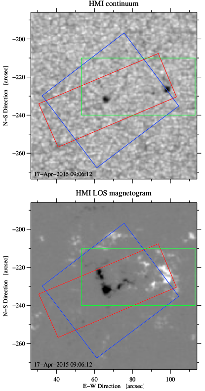
Figure 1: Overview of the EFR at 09:06 UT on 2015 April 17: SDO HMI continuum image (top) and HMI magnetogram (bottom). We depict the the FOV of GRIS (red), CRISP (blue), and of the NLFFF results in Fig. 4 (green).

This study is the continuation of González Manrique et al. (2017b, 2018), who studied the evolution of an AFS in He I. The goal of the present study is to follow the evolution of the plasma flows across several heights at the footpoints of an AFS.

2 Observations and data reduction

A small EFR, containing two pores with opposite polarities and an associated AFS in the chromosphere, was observed on 2015 April 17. The region of interest (ROI) is located at heliographic coordinates S19^∘ and W4^∘ ($\mu\equiv\cos\theta=0.97$). Two instruments placed at two telescopes were involved in this coordinated observing campaign: (1) the GREGOR Infrared Spectrograph (GRIS, Collados et al., 2012) located at the 1.5-meter GREGOR solar telescope (Schmidt et al., 2012) at Observatorio del Teide, Tenerife, Spain and (2) the CRisp Imaging Spectro-Polarimeter (CRISP, Scharmer et al., 2008) located at the Swedish Solar Telescope (SST, Scharmer et al., 2003) at Observatorio Roque de los Muchachos, La Palma, Spain. The overlap of the two field-of-views (FOV) of the instruments is shown in Fig. 1. The FOVs are aligned with a continuum image of the Helioseismic and Magnetic Imager (HMI, Scherrer et al., 2012; Schou et al., 2012) on board of the Solar Dynamics Observatory (SDO, Pesnell et al., 2012).

We applied the standard data reduction to the spatio-spectral data cubes of the very fast spectroscopic mode from GRIS (González Manrique et al., 2016, 2018). The wavelength calibration includes corrections of the solar gravity redshift and orbital-motion (see appendices A and B in Kuckein et al., 2012). Since telluric lines are present in our spectral range, the Doppler velocities computed in this study were retrieved from an absolute-scale wavelength calibrated array. The spectral region observed with GRIS comprises the photospheric Ca I 10839 Å and Si I 10827 Å lines, as well as the chromospheric He I 10830 Å triplet among others. González Manrique et al. (2017b, 2018) studied the same data set of GRIS in the very fast spectroscopic mode in the He I 10830 Å spectral line. This study builds on the results of the previously mentioned papers.

Five time-series were recorded with CRISP each consisting of ten data sets with full-Stokes measurements in the photospheric Fe I 6173 Å line and in the chromospheric Ca II 8542 Å line. The observations cover the evolution of the region between 08:47 UT and 9:20 UT with a FOV of $54\arcsec\times 54\arcsec$. The spectral sampling of the Fe I line consist of 19 wavelength positions with an equidistant step of 25 mÅ (spectral range $-225$ mÅ to $+225$ mÅ with respect to the central wavelength and a continuum position at $+525$ mÅ). The exposure time amounts to 33 ms for a single image (12 accumulations, 33 ms each).

The spectral sampling of the chromospheric Ca II line comprises 21 wavelength positions. The exposure time amounts also to 33 ms for a single image (6 accumulations, 33 ms each). Sequentially observing both lines yields a total cadence of about 50 s. The CRISPRED data pipeline (de la Cruz Rodríguez et al., 2015) was used for CRISP data, carrying out dark, flat-field, demodulation, prefilter corrections among others. The images were restored with Multi-Object Multi-Frame Blind Deconvolution (MOMFBD, van Noort et al., 2005) method, based on the algorithm by Löfdahl (2002).

At around 09:05 UT, strong downflow velocities occur near one pore. The $50^{\mathrm{th}}$ scan at 09:05:54 UT (see Fig. 2) was selected as a reference for the GRIS data because of the good seeing conditions. The corresponding data set of CRISP was taken at 09:05:27 UT, despite only fair seeing conditions prevailed at SST.

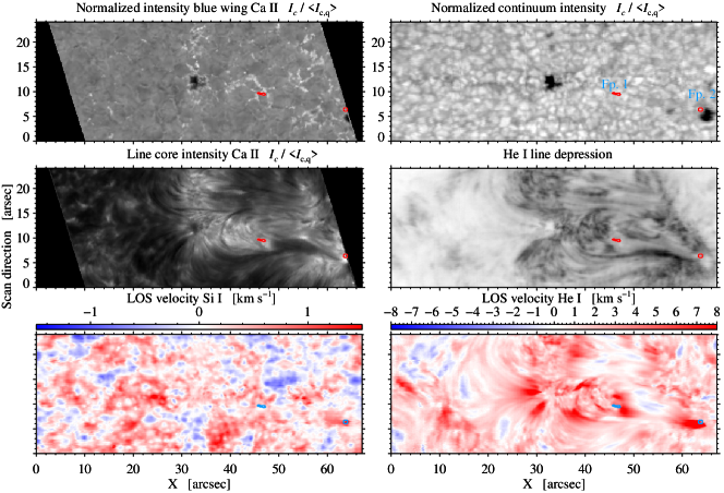
Figure 2: Restored CRISP images (top and middle left) at 09:05:27 UT and slit-reconstructed GRIS images (top and middle right) at 09:05:54 UT on 2015 April 17 of the EFR: blue wing of the chromospheric Ca II line (top left), continuum intensity observed with GRIS (top right), line core intensity of the chromospheric Ca II line (middle left), He I line depression (middle right), Si I Doppler velocity (bottom left), and He I Doppler velocity (bottom left). The red/blue contours depict the location of strong downflows at two different footpoints (Fp1 and Fp2). Black areas in the CRISP images indicate that there is no overlapping data with GRIS.

The HMI data were compensated for differential rotation with respect to the central meridian. The reference image was taken at 00:00:57 UT on 2015 April 17, considering that the position of the EFR was exactly at the central meridian.

3 Data analysis

A previous analysis of this data set was carried out for the Doppler velocities of the He I 10830 Å triplet by González Manrique et al. (2018). This triplet consists of one blue and two blended red components. A small proportion of spectral profiles contains apparent signatures of “dual flows” (Schmidt et al., 2000), which split the component into a slow and fast component. The single flow profiles of the red component of the He I triplet were fitted with a single Lorentzian. Furthermore, the dual-flow profiles were fitted with a double-Lorentzian profile. Details of the procedure on how to fit the two parts of the red component is explained in González Manrique et al. (2016, 2018).

The Si I 10827 Å, the Ca I 10839 Å, and the Fe I 6173 Å spectral lines were fitted with a Gaussian using the Levenberg-Marquardt least-squares minimization as implemented in the MPFIT IDL software package (Markwardt, 2009), to infer the respective LOS velocities at the core. The wavelength references for the LOS velocities were set to the laboratory wavelengths 10827.09 Å, 10838.97 Å, and 6173.33 Å, respectively, which were taken from the National Institute of Standards and Technology (NIST) database.

The information encoded in the chromospheric Ca II 8542 Å spectral line was analyzed using the non-LTE inversion code NICOLE (Socas-Navarro et al., 2015). The inversion process is complex and time-consuming for non-LTE lines. Hence, we concentrated only on a small region-of-interest (ROI) of 40 pixels (Fp. 1 in Fig. 2). This region was selected because we found strong chromospheric He I downflows during 30 minutes (almost one hour in the case of the Fp. 2 with 36 pixels, not inverted with NICOLE). We investigated also Fp. 2 because the He I Doppler velocities are higher than at Fp. 1 and the probability that the plasma reaches the photosphere is even higher at Fp. 2 compared to Fp. 1. The areas selected are represented by a red/blue contour in Fig. 2. The areas also depict the two regions with higher frequency of occurrence of He I dual-flow profiles during the observing period with GRIS (Fig. 5 in González Manrique et al., 2018). In some pixels we find persistently dual-flow profiles in 60 out of 64 He I maps. Since the aim is to retrieve the LOS velocities, we focused only on the inversion of the Stokes-$I$ profiles inside this region. For the inversions, we took into account the isotopic splitting of the Ca II NIR line (Leenaarts et al., 2014) and used the FALC model (Fontenla et al., 1993) as an initial estimate for the atmosphere.

To investigate the evolution of the three-dimensional (3D) magnetic topology of the AFS, we perform nonlinear force-free field (NLFFF) extrapolations by using the “weighted optimization” method (Wiegelmann, 2004; Wiegelmann et al., 2012). The boundary condition for the NLFFF extrapolation is given by an HMI photospheric vector magnetogram with an image scale of 0.5″ pixel^-1 which was preprocessed by a procedure developed by Wiegelmann et al. (2006) to satisfy the force-free condition. The NLFFF extrapolations are performed within a box of $224\,\times\,104\,\times\,128$ uniformly spaced grid points (about 81 $\,\times\,38\,\times\,46$ Mm³).

4 Results

In this study we investigate the height dependence of the draining flows along the arch filaments across different layers of the solar atmosphere, from the upper chromosphere down to the photosphere.

Following the plasma requires carefully selected spectral lines observed simultaneously, which form at different heights of the solar atmosphere and cover a large range of heights. In this case, two chromospheric and three photospheric spectral lines were used, combining two different ground-based telescopes.

We selected the two footpoints of a single arch filament (see Fp. 1 and Fp. 2 in Fig. 2). We computed the average Doppler velocities within the area of the contours of Fp. 1 and Fp. 2 in every map available with both instruments. In Fig. 3, we show the temporal evolution of the Doppler velocities for the He I red component, Ca II, and Si I.

The temporal evolution of the average Doppler velocities based on the He I triplet’s red component and the Si I spectral line of Fp. 2 is represented by blue and green bullets in the top right and bottom right panels of Fig. 3. Practically the entire CRISP data do not include the Fp. 2 area. Hence, it was impossible to calculate the evolution of the Doppler velocities at Fp. 2 based on the Ca II and Fe I spectral lines.

In both footpoints Fp. 1 and Fp. 2, the temporal evolution of the Doppler velocities based on the He I red component follows a similar pattern, showing peaks of high velocities at around 09:00 UT. The flows represent the evolution taking place in the upper layers of the chromosphere. Between 08:17 UT and 08:41 UT of the time-series observed with GRIS the average Doppler velocities varied in the range of 1 – 13 km s^-1 for Fp. 1 whereas Fp. 2 fluctuated between 7 – 19 km s^-1. Around 08:41 UT (dashed line in Fig. 3), the averaged Doppler velocities rapidly increased up to 20 and 24 km s^-1 at Fp. 1 (09:00 UT) and Fp. 2 (09:02 UT), respectively. At the end of the time-series, starting at 09:08 UT the Doppler velocities strongly dropped to 0 – 7 km s^-1 for Fp. 1 and 2 – 4km s^-1 for Fp. 2, respectively.

The temporal evolution between 08:47 UT and 09:20 UT of the mean Doppler velocities based on the Ca II is delineated by red bullets (in Fig. 3). The Doppler velocities at Fp. 1 were computed as averaged values within the range of $\log\tau\in[-2.4,-3.0]$ (red/blue contour in Fig. 2), corresponding to the upper photosphere. This range fits within the values of the computed response functions (RFs) by Quintero Noda et al. (2016) and Kuckein et al. (2017) for Ca II 8542 Å. The plot exhibits the same peak at around 09:00 UT as the He I Doppler shifts. The average Doppler velocities promptly increased up to 11 km s^-1 and then rapidly dropped to almost 0 km s^-1. Thus, we assume that the plasma moves along the leg of the arch filament at Fp. 1, from the upper to the lower chromosphere/upper photosphere with a clear deceleration.

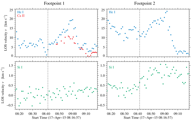
Figure 3: Temporal evolution of the average Doppler velocities of Fp. 1 (left) and Fp. 2 (right) as observed in the He I triplet red component (blue), the Ca II spectral line (red), and the Si I spectral line (see Fig. 2). The dashed vertical lines mark the time when the Doppler velocities suddenly increase.

The line core of the Si I spectral line is formed in the upper photosphere (e.g., Bard & Carlsson, 2008; Shchukina et al., 2017; Felipe et al., 2016). However, when computing the Doppler shifts with a Gaussian fit, we retrieve the average shift of the line. The LOS velocity evolution at Fp. 1 does not show any clear sign that the plasma reaches the upper photosphere at the Si I height formation (green bullets in Fig. 2). What we observe is likely the convection pattern with Doppler velocities varying between $\pm$0.5 km s^-1. Conversely, the velocity evolution at Fp. 2 shows an increase of the velocities measured in Si I co-temporal to the one exhibited by the He I triplet in the upper chromosphere. At the beginning of the time-series the velocity reaches up to 0.5 km s^-1. The velocity then rapidly increases at about the same time as the He I triplet (dashed line in Fig. 3) reaching velocities up to 1.5 km s^-1. Finally, the LOS velocities drop a few minutes later than in the upper chromosphere, at around 09:10 UT. The average Doppler velocities computed for the photospheric Fe I and Ca I photospheric spectral lines do not show any correlation with the strong downflows seen in the upper chromosphere.

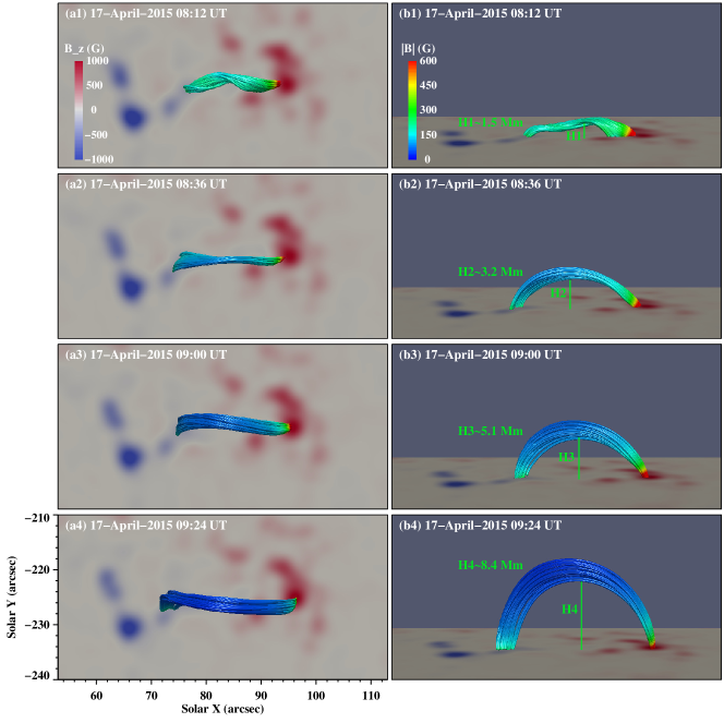
Figure 4: Magnetic structures revealed by NLFFF extrapolations for the arch filament studied in Fig. 3 connecting the footpoints Fp. 1 and Fp. 2 (Fig. 1). Four points in time were selected to compute the extrapolations: before the observations (top), first indications of the rising loop (second from top), during the time of the strongest Doppler velocities were detected as shown in Fig. 3 (third), and right after the observations (bottom). The photospheric vertical magnetograms ($B_{z}$) are displayed as background. The left panels depict the top view of the structures. The right panels show the side view. The colored loops illustrate the AFS magnetic fields. The different colors of the field lines depict the different values of the local magnetic field strength where red is the highest value.

The NLFFF extrapolations were modeled for four different times to associate the flows to the magnetic field topology (08:12 UT, 08:36 UT, 09:00 UT, and 09:24 UT). The time range covers our ground-based observing time. Figure 4 shows different perspectives of the extrapolation results. The colored loops represent how the estimated magnetic fields strength of the AFS evolve with time. Close to the beginning of the observations with GRIS, the extrapolations exhibit slightly twisted magnetic loops with maximum height of about 1.5 Mm. Approximately 24 and 48 minutes later, the magnetic loops are no longer twisted and the height increased up to 3.2 and 5.1 Mm respectively. At the end of the time-series, the height of the magnetic loop continued to increase up to 8.4 Mm. This confirms the hypothesis of González Manrique et al. (2018) concerning the evolution of an arch filament (see their Fig. 15). The scenario presented by these authors suggests step by step how the plasma rises from the photosphere to the chromosphere and even the corona. The sketch only represents the evolution as seen in the He I. In the first panels (Fig. 15) they described how the plasma rises from the photosphere to the chromosphere and the velocities at the loop tops reach their maximum upflow velocities. After a few minutes the material starts to drain along the legs towards the photosphere. This plasma accelerates reaching supersonic velocities. As seen in the last panels (Fig. 15), the arch filament continues rising to the transition region or even the corona. The downflows observed at the footpoints progressively decrease until they completely vanish. The NLFFF extrapolations and the LOS velocities presented in this study corroborate this scenario.

In Fig. 4, the field lines of the emerging magnetic loops were colored depending on the values of local magnetic field strength. This clearly shows strong magnetic fields at the footpoints and weaker fields at the loop tops. Interestingly, Fp. 2 exhibits higher values than the values computed at Fp. 1. This can be an important aspect to discern the downflow asymmetries between both footpoints (see Sect. 5).

5 Discussion and Conclusions

We scrutinized how the plasma flows along the footpoints of an AFS connecting two different polarities through different layers of the solar atmosphere. In both footpoints the dynamic shows similar LOS velocity pattern at different atmospheric layers, the upper chromosphere and the upper photosphere. This similar behavior of the plasma flows at different layers confirms that the plasma reached lower layers of the solar atmosphere coming from the upper chromosphere.

To confirm the plasma reaching the upper photosphere at Fp. 2, we used He I and Si I (GRIS), while at Fp. 1, we also used Ca II (CRISP). As we demonstrate in Fig. 3, we do not detect the plasma reaching the upper photosphere with the Doppler velocities inferred from the Si I spectral line at Fp. 1 while at Fp. 2 they are well detected. We expected to observe the same behaviour at Fp. 1 because the same LOS velocity pattern is identified in the upper photosphere with the Ca II spectral line. However, the Si I line is formed deeper in the atmosphere than the Ca II line and the fast flows have not reached the layers to which the Si I line is sensitive to. On the contrary, the plasma reaches deeper layers of the solar atmosphere at Fp. 2, compared to Fp. 1. We did not find any emission signatures in He I. The shocks manifest themselves in emission in this triplet. Therefore, there is no evidence for emission. Consequently, we cannot confirm that the plasma decelerates because of shocks produced below the He I height formation. A shock scenario cannot explain the downflow asymmetries in our case. We propose a different scenario based on the NLFFF extrapolations. The extrapolations (Fig. 4) do not show any obvious asymmetry of the rising loop, e.g., twist or an inclination angle. Furthermore, the extrapolations present different values of the magnetic field strength along the legs of the loops. The leg at Fp. 2 clearly has stronger magnetic fields $B$ (up to 600 G) than the leg at Fp. 1. Interestingly, the field lines at Fp. 2 are more compact or concentrated than those found at Fp. 1, which suggests a smaller cross-sectional area at Fp. 2. Hence, the magnetic field strength $B$ together with the cross-sectional areas $S$ are the key to understand the downflow asymmetries, as explained below.

We assume that the plasma moves from the chromosphere to the photosphere along a flux tube. The cross-sectional area $S$ of the tube is decreasing in the downward direction, and the plasma becomes denser. The plasma motion is governed by the equations of continuity, motion, and energy. The conservation of mass is given by the differential form of the continuity equation

$$\frac{\partial\rho}{\partial t}+\nabla(\rho v)=0,$$ (1)

where $\rho$ is the mass density and the Lagrangian derivative $d/dt\equiv\partial/\partial t+v\cdot\nabla$ was applied. If we also assume that the fluid is stationary $\partial\rho/\partial t=0$, the dynamic equilibrium is given by

$$\nabla(\rho v)=0.$$ (2)

If in addition the fluid moves along the field lines, then the equation simplifies to

$$\rho vS=c_{1},$$ (3)

where $S$ is the area enclosing the field lines, and $c_{1}$ is a constant. Similarly, one of Maxwell’s equations simplifies

$$\nabla B=0,$$ (4)

where $B$ is the magnetic field. If the magnetic flux is conserved then

$$BS=c_{2},$$ (5)

where $S$ is again the area enclosing the field lines, and $c_{2}$ is another constant.

Following the aforementioned equations, a plausible explanation for the flow asymmetries is that the values of the magnetic field $B$ are higher at Fp. 2 compared to Fp. 1. Stronger magnetic fields mean tighter field lines along this leg (the lower the height is, the stronger is the magnetic field $B$ and the cross-sectional area $S$ decreases). Consequently, the lower the height the smaller the cross section at Fp. 2 compared to Fp. 1. If we take into account the equations above (Eq. 3 and 5), together with the magnetic field values obtained from the extrapolations ($\sim$600 G at Fp. 2 versus $\sim$300 G at Fp. 1 at the level of the photosphere) and assuming that the density $\rho$ is similar at both footpoints, the velocities necessarily need to be higher (about two times higher) at Fp. 2 compared to Fp. 1. Since the field strength is stronger at Fp. 2, owing to the conservation of the flux across the flux tube the cross-sectional area $S$ needs to be smaller and hence the LOS velocities are higher at Fp. 2 than at Fp. 1. The photosperic Si I velocities measured at Fp. 1 are around $\pm$0.6 km s^-1 and between 0 km s^-1 and 1.5 km s^-1 at Fp. 2 (see Fig. 3). These values are in line with the proposed scenario. This explains the downflow asymmetries between both footpoints. In addition, it elucidates why the plasma slows down sooner along the leg of the AFS at Fp. 1 and does not reach the upper photosphere, as inferred from the Si I Doppler shifts, whereas at Fp. 2 we have evidence that the plasma reaches this height (as inferred from the Ca II inversions).

Downflows in arch filaments were explained by Chou (1993) as the emergence of a flux tube into the solar atmosphere. Lagg et al. (2007) proposed that the plasma carried by the rising loops drains to lower layers of the solar atmosphere along its legs because of the effect of gravity and the concurrent needs for vertical hydrostatic equilibrium and horizontal pressure balance. González Manrique et al. (2018) proposed that the arch filament carries plasma during the rise of the arch filament from the photosphere to the corona (see their sketch in Fig. 15). The authors suggested that after a certain time after the AFS starts rising, the plasma drains towards the photosphere along their legs reaching chromospheric supersonic velocities. Based on NLFFF extrapolations, we demonstrate that the magnetic field loops of the arch filament studied here rise with time (in about one hour) from 1.5 Mm up to 8.4 Mm, confirming the hypothesis of González Manrique et al. (2018) concerning the evolution of an arch filament. Interestingly, the loop reaches the largest height at 09:24 UT but the plasma flows already decline around 09:10 UT (with the maximum around 09:00 UT). We propose that the magnetic loop continues to rise but the plasma inside of the loop is evacuated before the magnetic loop reaches the corona. We observe that the He I absorption at the loop vanishes at the end of our observations (See the available movie in González Manrique et al. (2018)). Furthermore, we do not observe dual-flows anymore at the footpoints at the end of the observations (after 09:10 UT). Consequently, it is not possible to observe high velocities either because they do not exist any longer or because we cannot see them in the available spectral lines of this study.

References

- Avrett et al. (1994) Avrett, E. H., Fontenla, J. M., & Loeser, R. 1994, in IAU Symp., Vol. 154, Infrared Solar Physics, ed. D. M. Rabin, J. T. Jefferies, & C. Lindsey, 35
- Aznar Cuadrado et al. (2005) Aznar Cuadrado, R., Solanki, S. K., & Lagg, A. 2005, in ESA Spec. Publ., Vol. 596, Chromospheric and Coronal Magnetic Fields, ed. D. E. Innes, A. Lagg, & S. K. Solanki, 49.1
- Balthasar et al. (2016) Balthasar, H., Gömöry, P., González Manrique, S. J., et al. 2016, Astron. Nachr., 337, 1050, doi: 10.1002/asna.201612432
- Bard & Carlsson (2008) Bard, S., & Carlsson, M. 2008, ApJ, 682, 1376, doi: 10.1086/589910
- Bruzek (1967) Bruzek, A. 1967, Sol. Phys., 2, 451, doi: 10.1007/BF00146493
- Bruzek (1969) —. 1969, Sol. Phys., 8, 29, doi: 10.1007/BF00150655
- Chou (1993) Chou, D. Y. 1993, in ASP Conf. Ser., Vol. 46, IAU Colloq. 141: The Magnetic and Velocity Fields of Solar Active Regions, ed. H. Zirin, G. Ai, & H. Wang, 471–478
- Collados et al. (2012) Collados, M., López, R., Páez, E., et al. 2012, Astron. Nachr., 333, 872, doi: 10.1002/asna.201211738
- de la Cruz Rodríguez et al. (2015) de la Cruz Rodríguez, J., Löfdahl, M. G., Sütterlin, P., Hillberg, T., & Rouppe van der Voort, L. 2015, A&A, 573, A40, doi: 10.1051/0004-6361/201424319
- Diercke et al. (2019) Diercke, A., Kuckein, C., & Denker, C. 2019, A&A, 629, A48, doi: 10.1051/0004-6361/201935583
- Felipe et al. (2016) Felipe, T., Collados, M., Khomenko, E., et al. 2016, Astronomy and Astrophysics, 596, A59, doi: 10.1051/0004-6361/201629586
- Fontenla et al. (1993) Fontenla, J. M., Avrett, E. H., & Loeser, R. 1993, ApJ, 406, 319
- González Manrique et al. (2017a) González Manrique, S. J., Bello González, N., & Denker, C. 2017a, A&A, 600, A38, doi: 10.1051/0004-6361/201527880
- González Manrique et al. (2016) González Manrique, S. J., Kuckein, C., Pastor Yabar, A., et al. 2016, Astron. Nachr., 337, 1057
- González Manrique et al. (2017b) González Manrique, S. J., Denker, C., Kuckein, C., et al. 2017b, in IAU Symposium, Vol. 327, IAU Symposium, ed. S. Vargas Domínguez, A. G. Kosovichev, P. Antolin, & L. Harra, 28–33, doi: 10.1017/S1743921317000278
- González Manrique et al. (2018) González Manrique, S. J., Kuckein, C., Collados, M., et al. 2018, A&A, 617, A55, doi: 10.1051/0004-6361/201832684
- Kuckein et al. (2012) Kuckein, C., Martínez Pillet, V., & Centeno, R. 2012, A&A, 542, A112, doi: 10.1051/0004-6361/201218887
- Kuckein et al. (2017) Kuckein, C., Diercke, A., González Manrique, S. J., et al. 2017, A&A, 608, A117, doi: 10.1051/0004-6361/201731319
- Lagg et al. (2004) Lagg, A., Woch, J., Krupp, N., & Solanki, S. K. 2004, A&A, 414, 1109, doi: 10.1051/0004-6361:20031643
- Lagg et al. (2007) Lagg, A., Woch, J., Solanki, S. K., & Krupp, N. 2007, A&A, 462, 1147, doi: 10.1051/0004-6361:20054700
- Leenaarts et al. (2014) Leenaarts, J., de la Cruz Rodríguez, J., Kochukhov, O., & Carlsson, M. 2014, ApJ, 784, L17
- Löfdahl (2002) Löfdahl, M. G. 2002, in Proc. SPIE, Vol. 4792, Image Reconstruction from Incomplete Data, ed. P. J. Bones, M. A. Fiddy, & R. P. Millane, 146–155, doi: 10.1117/12.451791
- Markwardt (2009) Markwardt, C. B. 2009, in ASP Conf. Ser., Vol. 411, Astronomical Data Analysis Software and Systems XVIII, ed. D. A. Bohlender, D. Durand, & P. Dowler, 251–254
- Parker (1955) Parker, E. N. 1955, ApJ, 121, 491, doi: 10.1086/146010
- Pesnell et al. (2012) Pesnell, W. D., Thompson, B. J., & Chamberlin, P. C. 2012, Sol. Phys., 275, 3
- Quintero Noda et al. (2016) Quintero Noda, C., Shimizu, T., de la Cruz Rodríguez, J., et al. 2016, Mon. Not. R. Astron. Soc., 459, 3363
- Scharmer et al. (2003) Scharmer, G. B., Bjelksjo, K., Korhonen, T. K., Lindberg, B., & Petterson, B. 2003, in Proc. SPIE, Vol. 4853, Innovative Telescopes and Instrumentation for Solar Astrophysics, ed. S. L. Keil & S. V. Avakyan, 341–350
- Scharmer et al. (2008) Scharmer, G. B., Narayan, G., Hillberg, T., et al. 2008, ApJ, 689, L69
- Scherrer et al. (2012) Scherrer, P. H., Schou, J., Bush, R. I., et al. 2012, Sol. Phys., 275, 207
- Schmidt et al. (2000) Schmidt, W., Muglach, K., & Knölker, M. 2000, ApJ, 544, 567, doi: 10.1086/317169
- Schmidt et al. (2012) Schmidt, W., von der Lühe, O., Volkmer, R., et al. 2012, Astron. Nachr., 333, 796, doi: 10.1002/asna.201211725
- Schou et al. (2012) Schou, J., Scherrer, P. H., Bush, R. I., et al. 2012, Sol. Phys., 275, 229, doi: 10.1007/s11207-011-9842-2
- Shchukina et al. (2017) Shchukina, N. G., Sukhorukov, A. V., & Trujillo Bueno, J. 2017, A&A, 603, A98, doi: 10.1051/0004-6361/201630236
- Socas-Navarro et al. (2015) Socas-Navarro, H., de la Cruz Rodríguez, J., Asensio Ramos, A., Trujillo Bueno, J., & Ruiz Cobo, B. 2015, A&A, 577, A7
- Solanki et al. (2003) Solanki, S. K., Lagg, A., Woch, J., Krupp, N., & Collados, M. 2003, Nature, 425, 692, doi: 10.1038/nature02035
- Spadaro et al. (2004) Spadaro, D., Billotta, S., Contarino, L., Romano, P., & Zuccarello, F. 2004, A&A, 425, 309, doi: 10.1051/0004-6361:20041004
- Su et al. (2018) Su, Y., Liu, R., Li, S., et al. 2018, ApJ, 855, 77, doi: 10.3847/1538-4357/aaac31
- van Noort et al. (2005) van Noort, M., Rouppe van der Voort, L., & Löfdahl, M. G. 2005, Sol. Phys., 228, 191, doi: 10.1007/s11207-005-5782-z
- Wiegelmann (2004) Wiegelmann, T. 2004, Sol. Phys., 219, 87, doi: 10.1023/B:SOLA.0000021799.39465.36
- Wiegelmann et al. (2006) Wiegelmann, T., Inhester, B., & Sakurai, T. 2006, Sol. Phys., 233, 215, doi: 10.1007/s11207-006-2092-z
- Wiegelmann et al. (2012) Wiegelmann, T., Thalmann, J. K., Inhester, B., et al. 2012, Sol. Phys., 281, 37, doi: 10.1007/s11207-012-9966-z
- Xu et al. (2010) Xu, Z., Lagg, A., & Solanki, S. K. 2010, A&A, 520, A77, doi: 10.1051/0004-6361/200913227
- Zhong et al. (2019) Zhong, S., Hou, Y., Li, L., Zhang, J., & Xiang, Y. 2019, arXiv e-prints, arXiv:1907.10345. https://arxiv.org/abs/1907.10345
- Zwaan (1987) Zwaan, C. 1987, ARA&A, 25, 83, doi: 10.1146/annurev.aa.25.090187.000503