Operator product expansion coefficients in the exact renormalization group formalism

Abstract

We study how to compute the operator product expansion coefficients in the exact renormalization group formalism. After discussing possible strategies, we consider some examples explicitly, within the $\epsilon$-expansions, for the Wilson-Fisher fixed points of the real scalar theory in $d=4-\epsilon$ dimensions and the Lee-Yang model in $d=6-\epsilon$ dimensions. Finally we discuss how our formalism may be extended beyond perturbation theory.

I Introduction

The exact renormalization group (ERG) provides a framework to study the fundamental aspects of quantum field theories (QFT). For instance, it allows one to give a non-perturbative definition of renormalizable theories Wilson:1973jj and to discuss the realization of symmetries at the quantum level Igarashi:2009tj . On top of being a conceptual framework, ERG offers a framework for practical computations. It has been used as a computational tool for the universal quantities such as critical exponents in statistical field theory (see e.g. Berges:2000ew ; Delamotte:2007pf ), and also as an exploratory tool in a wide range of subjects including quantum gravity R96PaReut2018 .

Besides ERG, the operator product expansion (OPE) offers important insights into non-perturbative aspects of QFTs Wilson:1969zs . Let us denote composite operators as $\left[\mathcal{O}_{a}\right]$ and the product of two composite operators as $\left[\mathcal{O}_{a}\mathcal{O}_{b}\right]$. OPE states the validity of

$$\left[\mathcal{O}_{a}\left(x\right)\mathcal{O}_{b}\left(y\right)\right] =\sum_{c}C_{abc}\left(x-y\right)\left[\mathcal{O}_{c}\left(\frac{x+y}{2}\right)\right]$$ (1)

inserted into any correlation functions for small $|x-y|$. The existence of OPE has been proved perturbatively by Zimmermann Zimmermann:1972tv and plays a fundamental role in the study of conformal field theories (CFTs). Since both ERG and OPE offer non-perturbative insights into QFT, it is natural to study the relation between the two.

ERG was used to provide a perturbative proof of the existence of OPE Hughes:1988cp ; Keller:1991bz ; Keller:1992by ; Hollands:2011gf ; Holland:2014ifa ; Holland:2014pna , but little effort had been made to explore OPE within ERG beyond perturbation theory. In Pagani:2017tdr a non-perturbative definition of operator products was given, and simple examples of OPE were constructed in the Wilson action framework. Recently, composite operators have been constructed explicitly in the ERG formalism to make contact with various physical observables Becchi:1996an ; Igarashi:2009tj ; Rose:2015bma ; Rose:2016elj ; Daviet:2018lfy ; Pagani:2015hna ; Pagani:2016dof ; Becker:2018quq ; Becker2019Frank2020 .

In the present work we construct explicit examples of OPEs within the effective average action (EAA) framework Wetterich:1992yh . We identify two possible strategies to compute OPEs via ERG. One is based on the construction of operator products and their expansions in composite operators, and the other is based on the computation of three-point functions for theories with conformal invariance. We study explicit solutions of the ERG equations perturbatively with the $\epsilon$-expansions, and compare our results with those obtained via the conformal bootstrap Gaiotto:2013nva ; Hasegawa:2016piv ; Gopakumar:2016wkt ; Gopakumar:2016cpb ; Gopakumar:2018xqi . We also comment on how we may extend our strategies to non-perturbative approximation schemes available within the ERG formalism.

The paper is organized as follows. In section II we define composite operators and their products in the ERG formalism. We then consider the expansion of an operator product in composite operators and outline two possible strategies for the calculation of such an expansion. In section III we give technical remarks to explain how to construct operators at the Wilson-Fisher fixed point. Discussions of a fixed point require fixing a momentum cutoff, and we augment the technical outline given in section II where the momentum cutoff flows. Section IV is a long technical section, where we construct some composite operators explicitly and normalize them appropriately. In section V we apply the results obtained above to extract OPE coefficients and discuss our findings. We summarize our results in section VI and discuss the future perspectives.

II Operator product expansion in the ERG formalism

II.1 Operator products in the ERG

We extend the usual ERG formalism by introducing external sources that couple to composite operators so that the correlation functions of composite operators can be retrieved directly from the Wilson action. In this paper we actually prefer to discuss the 1PI counterpart of the Wilson action, known as the effective average action (EAA), so that we only need to deal with the 1PI part of the correlation functions which are relevant to the short distance singularities. A fully analogous construction applies to the Wilson action; see Pagani:2017tdr for example. For an overview regarding composite operators in the ERG formalism, we refer the reader to Becchi:1996an ; Pawlowski:2005xe ; Igarashi:2009tj ; Pagani:2016pad ; Pagani:2017tdr .

Let us consider the following modified generating functional of connected correlation functions:

$$Z_{k}\left[J,\varepsilon\right] =e^{W_{k}\left[J,\varepsilon\right]}$$

$$\equiv{\cal Z}\int{\cal D}\chi\,\exp\left[-S\left[\chi\right]+\int d^{d}x\,J\left(x\right)\chi\left(x\right)-\int d^{d}x\,\varepsilon_{i}\left(x\right)\mathcal{O}_{i}\left(x\right)-\Delta S_{k}\left[\chi\right]\right]\,,$$

where $S[\chi]$ is the bare action, and we have introduced the sources $J(x),\varepsilon_{i}(x)$ to the elementary field $\chi(x)$ and the composite operator $\mathcal{O}_{i}\left(x\right)$. The momentum $k$ is an IR cutoff, introduced via the IR cutoff action $\Delta S_{k}\left[\chi\right]$ defined by

$$\Delta S_{k}\left[\chi\right]\equiv\int d^{d}x\,\frac{1}{2}\chi\,{\cal R}_{k}\left(-\partial^{2}\right)\chi\,.$$

The kernel $\mathcal{R}_{k}\left(-\partial^{2}\right)\equiv k^{2}R\left(-\partial^{2}/k^{2}\right)$ suppresses the integration over the low momentum modes of $\chi$.

The EAA is then defined by the Legendre transform of $W_{k}\left[J,\varepsilon\right]$:

$$\Gamma_{k}\left[\varphi,\varepsilon\right]+\Delta S_{k}\left[\varphi\right]=\int d^{d}x\,J\left(x\right)\varphi\left(x\right)-W_{k}\left[J,\varepsilon\right]\,,$$

where

$$\varphi(x)=\frac{\delta W_{k}[J,\varepsilon]}{\delta J(x)}\,,$$

and no Legendre transform is performed over $\varepsilon$. A composite operator $\left[\mathcal{O}_{a}\right]\left(x\right)$ is defined by

$$\left[\mathcal{O}_{a}\right]\left(x\right)\equiv\frac{\delta\Gamma_{k}\left[\varphi,\varepsilon\right]}{\delta\varepsilon_{a}\left(x\right)}\Bigr{|}_{\varepsilon=0}\,.$$ (2)

This is motivated by its correspondence with $\frac{\delta}{\delta\varepsilon}Z_{k}$ at fixed source $J$. As a functional of $\varphi$, $\left[\mathcal{O}_{a}\right](x)$ gives the 1PI part of the correlation functions

$$\left\langle\left[\mathcal{O}_{a}\right](x)\chi(x_{1})\cdots\chi(x_{n})\right\rangle_{S}$$

in the limit $k\to 0$.

The product $\left[\mathcal{O}_{a}\mathcal{O}_{b}\right]\left(x,y\right)$ of two operators $\left[\mathcal{O}_{a}\right](x),\left[\mathcal{O}_{b}\right](y)$ is defined by

$$\left[\mathcal{O}_{a}\mathcal{O}_{b}\right]\left(x,y\right) \equiv-\frac{\delta^{2}\Gamma_{k}\left[\varphi,\varepsilon\right]}{\delta\varepsilon_{a}\left(x\right)\delta\varepsilon_{b}\left(y\right)}\Bigr{|}_{\varepsilon=0}+\int_{z_{1},z_{2}}\frac{\delta^{2}\Gamma_{k}[\varphi,\varepsilon]}{\delta\varepsilon_{b}\left(x\right)\delta\varphi\left(z_{1}\right)}\Bigr{|}_{\varepsilon=0}\cdot G_{k}\left(z_{1},z_{2}\right)\cdot\frac{\delta^{2}\Gamma_{k}[\varphi,\varepsilon]}{\delta\varphi\left(z_{2}\right)\delta\varepsilon_{b}\left(y\right)}\Bigr{|}_{\varepsilon=0}$$

$$\quad+\frac{\delta\Gamma_{k}[\varphi,\varepsilon]}{\delta\varepsilon_{a}\left(x\right)}\Bigr{|}_{\varepsilon=0}\frac{\delta\Gamma_{k}[\varphi,\varepsilon]}{\delta\varepsilon_{b}\left(y\right)}\Bigr{|}_{\varepsilon=0}\,,$$ (3)

where $G_{k}\left(z_{1},z_{2}\right)[\varphi]$ is the field dependent high-momentum propagator defined by

$$\int d^{d}x\,\frac{\delta^{2}\Gamma_{k}[\varphi,0]}{\delta\varphi(z_{1})\delta\varphi(x)}G_{k}\left(x,z_{2}\right)+\mathcal{R}_{k}\left(-\partial_{z_{1}}^{2}\right)G_{k}\left(z_{1},z_{2}\right)=\delta(z_{1}-z_{2})\,.$$ (4)

The product $\left[\mathcal{O}_{a}\mathcal{O}_{b}\right]\left(x,y\right)$ can be represented diagrammatically as in Fig. 1 which is motivated by its correspondence with $\frac{\delta^{2}}{\delta\varepsilon_{a}\delta\varepsilon_{b}}Z_{k}$ at fixed source $J$. See also Rose:2015bma .

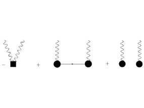
Figure 1: Diagrammatic representation of the full correlation function $\left[\mathcal{O}_{a}\mathcal{O}_{b}\right]$ in the EAA formalism. The black dots denote composite operators $\left[\mathcal{O}_{a}\right],\left[\mathcal{O}_{b}\right]$, i.e., the terms linear in the sources $\varepsilon$. The black square is the quadratic term $\frac{\delta^{2}\Gamma}{\delta\varepsilon_{a}\delta\varepsilon_{b}}\Bigr{|}_{\varepsilon=0}$.

Both $\left[\mathcal{O}_{a}\right]$ and $\left[\mathcal{O}_{a}\mathcal{O}_{b}\right]$ can be constructed from the associated ERG, as summarized below. The EAA $\Gamma_{k}\left[\varphi,\varepsilon\right]$ satisfies the ERG differential equation Wetterich:1992yh ; Ellwanger:1993mw ; Morris:1993qb ; Reuter:1993kw

$$\partial_{t}\Gamma_{k}\left[\varphi,\varepsilon\right]=\frac{1}{2}\mbox{Tr}\left[\left(\Gamma_{k}^{\left(2\right)}\left[\varphi,\varepsilon\right]+{\cal R}_{k}\right)^{-1}\partial_{t}{\cal R}_{k}\right]\,,$$ (5)

where

$$\partial_{t}\equiv-k\frac{\partial}{\partial k}\,,$$ (6)

and $\Gamma_{k}^{\left(2\right)}\left[\varphi,\varepsilon\right]=\frac{\delta^{2}\Gamma_{k}}{\delta\varphi\delta\varphi}$ is the Hessian of the EAA with respect to the average field. By taking the functional derivative of Eq. (5) we can derive the flow equations for composite operators and for the 1PI contributions to the operator products (3). More precisely, we obtain Pawlowski:2005xe ; Igarashi:2009tj ; Pagani:2016pad

$$\partial_{t}\left[\mathcal{O}_{a}\right]\left(x\right)=-\frac{1}{2}\mbox{Tr}\left[\left(\Gamma_{k}^{\left(2\right)}+{\cal R}_{k}\right)^{-1}\left[\mathcal{O}_{a}\right]^{\left(2\right)}\left(x\right)\left(\Gamma_{k}^{\left(2\right)}+{\cal R}_{k}\right)^{-1}\partial_{t}{\cal R}_{k}\right]\,,$$ (7)

where $\left[\mathcal{O}_{a}\right]^{\left(2\right)}=\frac{\delta^{2}}{\delta\varphi\delta\varphi}\left[\mathcal{O}_{a}\right]$ is the Hessian of the composite operator. For the products, we obtain

$$\partial_{t}\frac{\delta^{2}\Gamma_{k}\left[\varphi,\varepsilon\right]}{\delta\varepsilon_{a}\left(x\right)\delta\varepsilon_{b}\left(y\right)}\Bigr{|}_{\varepsilon=0}=-\frac{1}{2}\mbox{Tr}\left[\left(\Gamma_{k}^{\left(2\right)}+{\cal R}_{k}\right)^{-1}\frac{\delta^{2}\Gamma_{k}^{\left(2\right)}\left[\varphi,0\right]}{\delta\varepsilon_{a}\left(x\right)\delta\varepsilon_{b}\left(y\right)}\left(\Gamma_{k}^{\left(2\right)}+{\cal R}_{k}\right)^{-1}\partial_{t}{\cal R}_{k}\right]$$ (8)

$$\quad+\mbox{Tr}\left[\left(\Gamma_{k}^{\left(2\right)}+{\cal R}_{k}\right)^{-1}\frac{\delta\Gamma_{k}^{\left(2\right)}\left[\varphi,0\right]}{\delta\varepsilon_{a}\left(x\right)}\left(\Gamma_{k}^{\left(2\right)}+{\cal R}_{k}\right)^{-1}\frac{\delta\Gamma_{k}^{\left(2\right)}\left[\varphi,0\right]}{\delta\varepsilon_{b}\left(y\right)}\left(\Gamma_{k}^{\left(2\right)}+{\cal R}_{k}\right)^{-1}\partial_{t}{\cal R}_{k}\right]\,.$$

By solving Eqs. (7) and (8), we can construct the operator product $\left[\mathcal{O}_{a}\mathcal{O}_{b}\right]$ as in (3).

II.2 Operator product expansion coefficients in the ERG formalism

The operator product expansion (1) and its connection to ERG has already been studied in the literature Hughes:1988cp ; Keller:1991bz ; Keller:1992by ; Hollands:2011gf ; Holland:2014ifa ; Holland:2014pna ; Pagani:2017tdr . The ERG framework provides a further perturbative proof of the existence of the OPE Hughes:1988cp ; Keller:1991bz ; Keller:1992by ; Hollands:2011gf ; Holland:2014ifa ; Holland:2014pna . Actually, in the ERG formalism, the OPE (1) amounts to expressing the operator product $\left[\mathcal{O}_{a}\mathcal{O}_{b}\right]\left(x,y\right)$, given by (3), as an expansion in a basis of composite operators, given by (2). Thanks to the built-in locality, it has been argued that such an expansion is natural in the ERG formalism Pagani:2017tdr .

Let us emphasize that Eq. (1) is expected to hold along the entire RG trajectory. When the theory is at criticality, however, we expect

$$\Bigr{\langle}\left[\mathcal{O}_{a}\right]\left(x\right)\left[\mathcal{O}_{a}\right]\left(0\right)\Bigr{\rangle}=\frac{1}{\left|x-y\right|^{2\Delta_{a}}}$$ (9)

to be valid at large distances if the operators are normalized properly. Then, the OPE coefficients in (1) are given by

$$C_{abc}\left(x-y\right)=\frac{c_{abc}}{\left|x-y\right|^{\Delta_{a}+\Delta_{b}-\Delta_{c}}}\,,$$ (10)

where $\Delta_{a}$ is the scale dimension of the operator $\left[\mathcal{O}_{a}\right]$, and $c_{abc}$ is a numerical factor. We refer to this numerical factor $c_{abc}$ as an OPE coefficient. Theories with conformal symmetry are the IR limit of such critical theories, and the OPE coefficient $c_{abc}$ appears as the overall coefficient of the three-point function

$$\Bigr{\langle}\left[\mathcal{O}_{a}\right]\left(x_{1}\right)\left[\mathcal{O}_{b}\right]\left(x_{2}\right)\left[\mathcal{O}_{c}\right]\left(x_{3}\right)\Bigr{\rangle}=\frac{c_{abc}}{\left(x_{12}^{2}\right)^{d/2-\nu_{c}}\left(x_{23}^{2}\right)^{d/2-\nu_{a}}\left(x_{12}^{2}\right)^{d/2-\nu_{b}}}\,,$$ (11)

where $x_{ij}^{2}=\left|x_{i}-x_{j}\right|^{2}$, $c_{abc}$ is fully symmetric in its indices, and $\nu_{a}=\frac{1}{2}\left(d+\Delta_{a}-\Delta_{b}-\Delta_{c}\right)$, etc.

The main aim of this paper is to lay down a possible strategy for computing the OPE coefficients $c_{ijk}$ within the ERG framework. We can consider the following two possibilities.

A)

Construct the full operator product $\left[\mathcal{O}_{a}\mathcal{O}_{b}\right]$ first, and expand it in a basis of composite operators $\left[\mathcal{O}_{c}\right]$.

B)

Assuming conformal symmetry, extract the coefficient $c_{abc}$ directly from the three-point function given by (11).

The strategy A) has been followed in Pagani:2017tdr to provide simple examples around the Gaussian fixed point. Although available in principle, this strategy is cumbersome in practice. Since one usually works in momentum space, it is easier to construct the most singular (i.e., non-integrable) part of the OPE rather than the full (i.e., including the finite part) OPE.

In this paper we will consider the approach B) in detail within the ERG formalism. We will extract OPE coefficients from the associated three-point functions. We calculate in momentum space rather than in coordinate space. In subsection II.3 below we recall a few basic features of conformal invariance in momentum space and explain the main points of our recipe. As a side note, we point out that ERG is a very efficient framework to discuss the presence of conformal invariance Delamotte:2015aaa ; Delamotte:2018fnz ; DePolsi:2018vxc ; DePolsi:2019owi ; Rosten:2016nmc ; Rosten:2017urs ; Sonoda:2017zgl .

We apply the strategy outlined above to compute some examples of the OPE coefficients. We solve the ERG differential equations perturbatively and express the results via the $\epsilon$-expansion. This allows us to compare our results with others that have been obtained in the literature by means of the analytic conformal bootstrap approach Gaiotto:2013nva ; Hasegawa:2016piv ; Gopakumar:2016wkt ; Gopakumar:2016cpb ; Gopakumar:2018xqi . In particular, we will compute the coefficients “$c_{112}$” and “$c_{114}$” to the first order in $\epsilon$ for the critical Ising model in $d=4-\epsilon$ dimensions, and the coefficient “$c_{111}$” to the first order in $\sqrt{\epsilon}$ for the critical Lee-Yang model in $d=6-\epsilon$ dimensions. Our results agree with those obtained by other approaches.

II.3 Operator product expansion coefficients in momentum space

Calculations in quantum field theory often rely on momentum space, where the loop corrections are most easily expressed and computed. On the other hand, formulas regarding OPE are often most naturally expressed in real (coordinate) space, especially in the case of CFTs. In this subsection we briefly describe the connection between expressions in real space and those in momentum space.

Conformal symmetry in momentum space has been analyzed in the literature in some detail; see Coriano:2013jba ; Maglio:2019grh ; Bzowski:2013sza ; Bzowski:2015pba ; Bzowski:2015yxv ; Bzowski:2019kwd ; Isono:2019ihz ; Gillioz:2018mto and references therein. We only need a few very basic formulas, which we review below (a few more technical details are provided in Appendix A). We refer the interested reader to the literature given above for more details regarding the constraint imposed by conformal symmetry in momentum space.

Let us consider a set of primary operators $\phi_{i}$, normalized by the two-point functions

$$\left\langle\phi_{i}\left(x\right)\phi_{j}\left(0\right)\right\rangle=\frac{1}{x^{\Delta_{i}+\Delta_{j}}}\delta_{ij}\,.$$ (12)

In momentum space this normalization gives

$$\left\langle\phi_{i}\left(p\right)\phi_{i}\left(q\right)\right\rangle=(2\pi)^{d}\delta(p+q)\cdot\pi^{d/2}\frac{\Gamma\left(\frac{d}{2}-\Delta_{i}\right)}{\Gamma(\Delta_{i})}\left(\frac{4}{p^{2}}\right)^{\frac{d}{2}-\Delta_{i}}\,,$$ (13)

where we have used (119) given in Appendix A.

The Fourier transform of the three-point function

$$\left\langle\phi_{1}(x_{1})\phi_{2}(x_{2})\phi_{3}(x_{3})\right\rangle=\frac{c_{123}}{(x_{12}^{2})^{d/2-\nu_{3}}(x^{2}_{23})^{d/2-\nu_{1}}(x^{2}_{12})^{d/2-\nu_{2}}}$$ (14)

(the same as (11)) is given by a somewhat complicated expression either as a momentum integral or via special functions. To avoid such complications, we consider the limit $p_{1}\gg p_{2}$, where we find

$$\left\langle\phi_{1}\left(p_{1}\right)\phi_{2}\left(p_{2}\right)\phi_{3}\left(-p\right)\right\rangle\overset{p_{1}\gg p_{2}}{\longrightarrow}(2\pi)^{d}\delta(p_{1}+p_{2}-p)\cdot\frac{c_{123}}{p_{1}^{d+\Delta_{2}-\Delta_{1}-\Delta_{3}}p_{2}^{d-2\Delta_{2}}}$$

$$\quad\times\left(4\pi\right)^{d}4^{-\frac{1}{2}\left(\Delta_{1}+\Delta_{2}+\Delta_{3}\right)}\frac{\Gamma\left(\frac{1}{2}\left(d+\Delta_{2}-\Delta_{1}-\Delta_{3}\right)\right)}{\Gamma\left(\frac{1}{2}\left(\Delta_{1}+\Delta_{3}-\Delta_{2}\right)\right)}\frac{\Gamma\left(\frac{d}{2}-\Delta_{2}\right)}{\Gamma\left(\Delta_{2}\right)}\,.$$ (15)

To extract the coefficient $c_{123}$, it is enough to know this asymptotic behavior . We provide a little more details of this formula in Appendix A.

III Wilson-Fisher fixed point

In this section we wish to discuss technicalities that are quite important for our calculations. In the main part of this paper we consider a real scalar theory at its criticality in $d=4-\epsilon$ dimensions. In doing so with ERG, we have two alternatives:

C)

We start from a bare theory $S_{B}[\chi]$ with a large but finite cutoff $k_{0}$. We tune the bare parameters to make the theory critical. We then construct the EAA $\Gamma_{k}[\varphi,\varepsilon]$ whose $k$-dependence is determined by ERG. In the limit $k\to 0$, $\Gamma_{k}$ becomes the 1PI generating functional of the correlation functions. A conformal field theory is obtained as the IR limit of the critical theory, i.e., we must look at the correlation functions for the momenta much smaller than the bare cutoff $k_{0}$.

D)

We adopt the dimensionless convention by measuring all dimensionful quantities in appropriate powers of the cutoff $k$. The resulting 1PI EAA $\bar{\Gamma}_{t}[\bar{\varphi},\bar{\varepsilon}]$ has a fixed cutoff of order $1$, and satisfies an ERG differential equation with the Gaussian and Wilson-Fisher fixed-point solutions. $\bar{\Gamma}_{*}[\bar{\varphi},\bar{\varepsilon}]$ at the Wilson-Fisher fixed point gives the correlation functions of a conformal field theory, but only for the momenta much larger than the fixed cutoff.Sonoda:2017rro

We prefer D) because it is easier to construct a fixed point than to tune a bare theory for criticality. For completeness and the convenience of the reader, let us rewrite the relevant ERG differential equations in the dimensionless convention.

We first introduce dimensionless fields by

$$\bar{\varphi}(p) \equiv k^{\frac{d+2}{2}}\varphi(pk)\,,$$ (16a)

$$\left[\bar{\mathcal{O}}_{i}\right](p) \equiv k^{d-d_{i}}\left[\mathcal{O}_{i}\right](pk)\,,$$ (16b)

$$\bar{\varepsilon}_{i}(p) \equiv k^{d_{i}}\varepsilon_{i}(pk)\,,$$ (16c)

where $d_{i}$ is the scale dimension of $\left[\mathcal{O}_{i}\right](x)=\int_{p}e^{ipx}\left[\mathcal{O}_{i}\right](p)$ in the coordinate space at the Gaussian fixed point. It is sometimes called the engineering dimension.

We then define

$$\bar{\Gamma}_{t}[\bar{\varphi},\bar{\varepsilon}]\equiv\Gamma_{k}[\varphi,\varepsilon]\,,$$ (17)

where we have traded the momentum cutoff $k$ for the logarithmic flow time $t$, given by (6). The ERG differential equation for $\bar{\Gamma}_{t}[\bar{\varphi},\bar{\varepsilon}]$ is given by

$$\partial_{t}\bar{\Gamma}_{t}[\bar{\varphi},\bar{\varepsilon}] =\int_{p}\left(\frac{d+2}{2}+p\cdot\partial_{p}\right)\bar{\varphi}(p)\cdot\frac{\delta\bar{\Gamma}_{t}[\bar{\varphi},\bar{\varepsilon}]}{\delta\bar{\varphi}(p)}+\int_{p}\left(d_{i}+p\cdot\partial_{p}\right)\bar{\varepsilon}_{i}(p)\cdot\frac{\delta\bar{\Gamma}_{t}[\bar{\varphi},\bar{\varepsilon}]}{\delta\bar{\varepsilon}_{i}(p)}$$

$$\quad-\int_{p}\left(2-p\cdot\partial_{p}\right)R(p)\cdot\frac{1}{2}G_{t;p,-p}[\bar{\varphi},\bar{\varepsilon}]\,,$$ (18)

where $G_{t;p,-q}[\bar{\varphi},\bar{\varepsilon}]$ is defined by

$$\int_{q}G_{t;p,-q}[\bar{\varphi},\bar{\varepsilon}]\left(\frac{\delta^{2}\bar{\Gamma}_{t}[\bar{\varphi},\bar{\varepsilon}]}{\delta\bar{\varphi}(q)\delta\bar{\varphi}(-r)}+R(q)\,(2\pi)^{d}\delta(q-r)\right)=(2\pi)^{d}\delta(p-r)\,.$$ (19)

The cutoff function $R(q)$ is a fixed function.

We are interested in the ERG flow from the Gaussian fixed point to the Wilson-Fisher fixed point. We parametrize the flow by $g$ so that the Gaussian fixed point is at $g=0$, and the Wilson-Fisher fixed point is at $g=g_{*}$. We can then replace $\partial_{t}$ by

$$\left(\epsilon g+\beta(g)\right)\partial_{g}$$

where $\epsilon$ is the scale dimension of $g$ at $g=0$. Accordingly, $\bar{\Gamma}(g)[\bar{\varphi}]=\bar{\Gamma}_{t}[\bar{\varphi},0]$ satisfies the ERG equation

$$\left\{\left(\epsilon g+\beta(g)\right)\partial_{g}+\Delta_{\bar{\varphi}}\right\}\bar{\Gamma}(g)[\bar{\varphi}]=-\int_{p}\left(2-p\cdot\partial_{p}\right)R(p)\cdot\frac{1}{2}G(g)_{p,-p}[\bar{\varphi}]\,,$$ (20)

where we define $\Delta_{\bar{\varphi}}$ and $G(g)_{p,-q}[\bar{\varphi}]$ by

$$\Delta_{\bar{\varphi}}\equiv\int_{p}\left(-\frac{d+2}{2}-p\cdot\partial_{p}\right)\bar{\varphi}(p)\cdot\frac{\delta}{\delta\bar{\varphi}(p)}\,,$$ (21)

and

$$\int_{q}G(g)_{p,-q}[\bar{\varphi}]\left(\frac{\delta^{2}\bar{\Gamma}(g)[\bar{\varphi}]}{\delta\bar{\varphi}(q)\delta\bar{\varphi}(-r)}+R(q)\,(2\pi)^{d}\delta(q-r)\right)=(2\pi)^{d}\delta(p-r)\,.$$ (22)

Actually, for the Wilson-Fisher fixed point to exist at $g=g_{*}=\mathrm{O}(\epsilon)$, we need to introduce an anomalous dimension $\frac{1}{2}\eta(g)=\mathrm{O}(g^{2})$ of $\bar{\varphi}$. Since we are only interested in the corrections of order $\epsilon$ to the OPE coefficients, we can ignore it. In Appendix B we obtain $\beta(g)$ to order $g^{2}$ to determine the fixed-point value

$$g_{*}=\frac{(4\pi)^{2}}{3}\epsilon+\mathrm{O}(\epsilon^{2})\,.$$ (23)

Similarly, differentiating (18) with respect to $\bar{\epsilon}_{i}$, we obtain the ERG equation for $\left[\bar{\mathcal{O}}_{i}\right]$ as

$$\left\{\left(\epsilon g+\beta(g)\right)\partial_{g}+d-d_{i}+p\cdot\partial_{p}+\Delta_{\bar{\varphi}}\right\}\left[\bar{\mathcal{O}}_{i}\right](p)-\sum_{j}\gamma_{ij}(g)\left[\bar{\mathcal{O}}_{j}\right](p)$$

$$=\int_{q}(2-q\cdot\partial_{q})R(q)\,\frac{1}{2}\int_{r,s}G(g)_{q,-r}[\bar{\varphi}]\frac{\delta^{2}\left[\bar{\mathcal{O}}_{i}\right](p)}{\delta\bar{\varphi}(r)\delta\bar{\varphi}(s)}G(g)_{-s,-q}[\bar{\varphi}]\,.$$ (24)

The mixing matrix $\gamma_{ij}(g)$ results from appropriate boundary conditions imposed at $p=0$. Differentiating (18) once more, we obtain the ERG equation for

$$\mathcal{Q}_{ij}(p_{1},p_{2})\equiv-\frac{\delta^{2}\bar{\Gamma}(g)[\bar{\varphi},\bar{\varepsilon}]}{\delta\bar{\varepsilon}_{i}(-p_{1})\delta\bar{\varepsilon}_{j}(-p_{2})}\Bigr{|}_{\varepsilon=0}$$ (25)

as

$$\left\{\left(\epsilon g+\beta(g)\right)\partial_{g}+2d-d_{i}-d_{j}+p_{1}\cdot\partial_{p_{1}}+p_{2}\cdot\partial_{p_{2}}+\Delta_{\bar{\varphi}}\right\}\mathcal{Q}_{ij}(p_{1},p_{2})$$

$$\quad-\sum_{k}\left(\gamma_{ik}(g)\mathcal{Q}_{kj}(p_{1},p_{2})+\gamma_{jk}(g)\mathcal{Q}_{ik}(p_{1},p_{2})+\gamma_{ij,k}(g)\left[\bar{\mathcal{O}}_{k}\right](p_{1}+p_{2})\right)$$

$$=\int_{q}\left(2-q\cdot\partial_{q}\right)R(q)\,\int_{r,s}G(g)_{q,-r}[\bar{\varphi}]G(g)_{s,-q}[\bar{\varphi}]$$

$$\quad\times\left(\frac{1}{2}\frac{\delta^{2}\mathcal{Q}_{ij}(p_{1},p_{2})}{\delta\bar{\varphi}(r)\delta\bar{\varphi}(-s)}+\int_{u,v}\frac{\delta^{2}\left[\bar{\mathcal{O}}_{i}\right](p_{1})}{\delta\bar{\varphi}(r)\delta\bar{\varphi}(-u)}G(g)_{u,-v}[\bar{\varphi}]\frac{\delta^{2}\left[\bar{\mathcal{O}}_{j}\right](p_{2})}{\delta\bar{\varphi}(v)\delta\bar{\varphi}(-s)}\right)\,,$$ (26)

where the mixing $\gamma_{ij,k}(g)$ is due to appropriate boundary conditions imposed at $p_{1}=p_{2}=0$.

We have thus given the defining ERG differential equations for $\bar{\Gamma}(g)[\bar{\varphi}]$, $\left[\bar{\mathcal{O}}_{i}\right](g;p)$, and $\mathcal{Q}_{ij}(g;p_{1},p_{2})$. We end this section by summarizing how to extract the two- and three-point functions out of these Sonoda:2017rro . We first set $g$ to the fixed-point value $g_{*}$ to go to the Wilson-Fisher fixed point. To extract the two-point function of the elementary scalar field, we expand

$$\bar{\Gamma}(g_{*})[\bar{\varphi}]=\frac{1}{2}\int_{p_{1},p_{2}}\bar{\varphi}(p_{1})\bar{\varphi}(p_{2})\,(2\pi)^{d}\delta(p_{1}+p_{2})\,\bar{\Gamma}^{(2)}(p_{1})+\cdots$$ (27)

in powers of fields. For $p\gg 1$, we obtain the two-point function as

$$\left\langle\bar{\varphi}(p)\bar{\varphi}(q)\right\rangle=\frac{1}{\bar{\Gamma}^{(2)}(p)}\,(2\pi)^{d}\delta(p+q)\,.$$ (28)

Similarly, the field independent part of

$$\left[\bar{\mathcal{O}}_{i}\bar{\mathcal{O}}_{j}\right](g_{*};p_{1},p_{2})=\left[\bar{\mathcal{O}}_{i}\bar{\mathcal{O}}_{j}\right]^{(0)}(p_{1})\,(2\pi)^{d}\delta(p_{1}+p_{2})+\cdots$$ (29)

gives, for $p_{1},p_{2}\gg 1$, the two-point function as

$$\left\langle\bar{\mathcal{O}}_{i}(p_{1})\bar{\mathcal{O}}_{j}(p_{2})\right\rangle=\left[\bar{\mathcal{O}}_{i}\bar{\mathcal{O}}_{j}\right]^{(0)}(p_{1})\,(2\pi)^{d}\delta(p_{1}+p_{2})\,.$$ (30)

Finally, the part quadratic in fields of

$$\left[\bar{\mathcal{O}}_{i}\right](g_{*};p)=\frac{1}{2}\int_{p_{1},p_{2}}\bar{\varphi}(p_{1})\bar{\varphi}(p_{2})\,(2\pi)^{d}\delta(p_{1}+p_{2}-p)\,\left[\bar{\mathcal{O}}_{i}\right]^{(2)}(p_{1},p_{2})+\cdots$$ (31)

gives, for $p_{1},p_{2}\gg 1$, the three-point function as

$$\left\langle\bar{\varphi}(-p_{1})\bar{\varphi}(-p_{2})\bar{\mathcal{O}}_{i}(p)\right\rangle=\left[\bar{\mathcal{O}}_{i}\right]^{(2)}(p_{1},p_{2})\frac{1}{\bar{\Gamma}^{(2)}(p_{1})\bar{\Gamma}^{(2)}(p_{2})}\,(2\pi)^{d}\delta(p_{1}+p_{2}-p)$$ (32)

for $\mathbb{Z}_{2}$-invariant operators $\left[\bar{\mathcal{O}}_{i}\right]$. This equation needs to be modified as (115) if the fixed point has no $\mathbb{Z}_{2}$ invariance.

In the remaining part of the paper we work only in the dimensionless convention. Hence, we omit the bars above the symbols altogether.

IV Scaling operators from ERG

In this section we construct explicitly scaling composite operators $\phi_{i}$ at the Wilson-Fisher fixed point in $d=4-\epsilon$ dimensions by solving the ERG. Composite operators are solutions of (24), which we write again as

$$\left(p\cdot\partial_{p}+\Delta_{\varphi}\right)\left[\mathcal{O}_{i}\right](p)+\left(d\,\delta_{ij}-\Delta_{ij}\right)\left[\mathcal{O}_{j}\right](p)$$

$$=\frac{1}{2}\int_{q}(2-q\cdot\partial_{q})R(q)\int_{r,s}G_{q,-r}[\Phi]G_{-q,-s}[\Phi]\frac{\delta^{2}\left[\mathcal{O}_{i}\right](p)}{\delta\varphi(r)\delta\varphi(s)}\,,$$ (33)

where $G_{p,q}[\Phi]$ is defined by

$$\int_{q}G_{p,q}[\Phi]\left(\frac{\delta^{2}\Gamma_{*}[\varphi]}{\delta\varphi(-q)\delta\varphi(r)}+R(q)(2\pi)^{d}\delta(q-r)\right)=(2\pi)^{d}\delta(p-r)\,,$$

and

$$\Delta_{\varphi}\equiv\int_{q}\left(-\frac{d+2}{2}-q\cdot\partial_{q}\right)\varphi(q)\cdot\frac{\delta}{\delta\varphi(q)}\,.$$

$\Delta_{ij}$ is the matrix of scale dimensions, and it is not diagonal in general:

$$\Delta_{ij}=d_{i}\,\delta_{ij}+\gamma_{ij}\,,$$

where $d_{i}$ is the engineering (mass) dimension of $\mathcal{O}_{i}$ in coordinate space, and $\gamma_{ij}$ is the mixing matrix.

The scaling composite operators $\phi_{i}$ are suitable linear combinations of composite operators that diagonalize the mixing matrix $\Delta_{ij}$. The scaling operators $\left[\Phi_{i}\right]$ for the eigenvalue $\Delta_{i}$ satisfy

$$\left(p\cdot\partial_{p}+d-\Delta_{i}+\Delta_{\varphi}\right)\left[\Phi_{i}\right](p)$$

$$=\frac{1}{2}\int_{q}(2-q\cdot\partial_{q})R(q)\int_{r,s}G_{q,-r}[\varphi]G_{-q,-s}[\varphi]\frac{\delta^{2}\left[\Phi_{i}\right](p)}{\delta\varphi(r)\delta\varphi(s)}\,.$$ (34)

We can then introduce a normalization constant $\mathcal{N}_{i}$ so that $\phi_{i}\equiv{\cal N}_{i}\left[\Phi_{i}\right]$ satisfies the normalization (12). Note that the coefficient ${\cal N}_{i}$ depends on the space dimension $d$, and therefore on $\epsilon$. Possibly, the simplest example along this line is given by the field $\phi_{1}\equiv{\cal N}_{1}\varphi$, which we describe in section IV.1.

Of course, before solving the ERG for the composite operators and their products, we need to solve the ERG equation to obtain $\Gamma_{*}[\varphi]$ at the fixed point. In this work we use perturbation theory to solve the ERG explicitly. Since solving for $\Gamma_{*}\left[\varphi\right]$ is not the main focus of this paper, we give the first order derivation of $\Gamma_{*}[\varphi]$ in Appendix B. For the present purposes, it suffices to say that the EAA parametrized by $g$ is expressed as

$$\Gamma(g)[\varphi] =\frac{1}{2}\int_{p}\varphi(p)\varphi(-p)v^{(2)}(g;p)$$

$$\quad+\frac{1}{4!}\int_{p_{1},\cdots,p_{4}}\prod_{i=1}^{4}\varphi(p_{i})\,(2\pi)^{d}\delta\left(\sum_{i=1}^{4}p_{i}-p\right)\,v^{(4)}(g;p_{1},\cdots,p_{4})\,,$$ (35)

where

$$v^{(2)}(g;p) =p^{2}+gv_{1}^{(2)}\,,$$ (36a)

$$v^{(4)}(g;p_{1},\cdots,p_{4}) =g+g^{2}v_{2}^{(4)}(p_{1},\cdots,p_{4})\,.$$ (36b)

$v_{1}^{(2)}$ is a constant given by (140), and the momentum dependent $v_{2}^{(4)}$ is given by (144). The Wilson-Fisher fixed point corresponds to $g=g_{*}=\frac{(4\pi)^{2}}{3}\epsilon$ up to order $\epsilon$. We introduce the high momentum propagator and its derivative by

$$h(p) \equiv\frac{1}{p^{2}+R(p)}\,,$$ (37a)

$$f(p) \equiv(p\cdot\partial_{p}+2)h(p)=\frac{(2-p\cdot\partial_{p})R(p)}{\left(p^{2}+R(p)\right)^{2}}\,.$$ (37b)

Both $R(p)$ and $f(p)$ decay rapidly at $p\gg 1$. To second order in $g$ the beta function is given by

$$\beta(g)=\beta_{2}\,g^{2}=\left(-3\int_{q}f(q)h(q)\right)g^{2}\,,$$ (38)

where

$$\int_{q}f(q)h(q)=\frac{1}{(4\pi)^{2}}+\mathrm{O}(\epsilon)\,.$$ (39)

Using this result, calculated in Appendix C, we obtain $g_{*}$ given in (23).

IV.1 The scaling field $\phi_{1}$

To first order in $g$, we obtain

$$\Gamma^{(2)}(g;p,-p)=p^{2}+gv_{1}^{(2)}$$ (40)

where

$$v_{1}^{(2)}=\frac{1}{2-\epsilon}\int_{q}f(q)$$ (41)

is a constant. As $p\to\infty$, we obtain

$$\Gamma^{(2)}(g;p,-p)\overset{p\to\infty}{\longrightarrow}p^{2}\,.$$ (42)

Hence, to first order in $g$, the two-point function is the same as the Gaussian theory:

$$\left\langle\varphi(p)\varphi(q)\right\rangle=\frac{1}{p^{2}}\,(2\pi)^{d}\delta(p+q)\,.$$ (43)

Taking the inverse Fourier transform, we obtain

$$\left\langle\varphi(r)\varphi(0)\right\rangle=\frac{1}{\mathcal{N}_{1}^{2}}\frac{1}{r^{d-2}}\,,$$ (44)

where

$$\frac{1}{\mathcal{N}_{1}^{2}}\equiv\frac{1}{4\pi^{\frac{d}{2}}}\Gamma\left(\frac{d-2}{2}\right)\,.$$ (45)

(See Appendix A.) Thus, $\phi_{1}=\mathcal{N}_{1}\varphi$ has the normalization of (12).

IV.2 The composite operator $\left[\varphi^{2}/2\right]$

In this subsection we construct the composite operator $\left[\varphi^{2}/2\right]$. This satisfies the ERG equation

$$\left\{\left(\epsilon g+\beta(g)\right)\partial_{g}+p\cdot\partial_{p}+2+\Delta_{\varphi}\right\}\left[\frac{1}{2}\varphi^{2}\right](p)=\gamma_{2}(g)\left[\frac{1}{2}\varphi^{2}\right](p)$$

$$\quad+\int_{q}(2-q\cdot\partial_{q})R(q)\frac{1}{2}\int_{r,s}G(g)_{q,-r}G(g)_{-s,-q}\frac{\delta^{2}}{\delta\varphi(r)\delta\varphi(s)}\left[\frac{1}{2}\varphi^{2}\right](p)\,,$$ (46)

where $\gamma_{2}(g)$ is the anomalous dimension. To solve this, we expand the operator in powers of $\varphi$:

$$\left[\frac{1}{2}\varphi^{2}\right](p)=\sum_{n=0}^{\infty}\frac{1}{(2n)!}\int_{p_{1},\cdots,p_{2n}}\prod_{i=1}^{2n}\varphi(p_{i})\cdot(2\pi)^{d}\delta\left(\sum_{i=1}^{2n}p_{i}-p\right)\,c^{(2n)}(g;p_{1},\cdots,p_{2n})\,.$$ (47)

We normalize the operator by the condition

$$c^{(2)}(g;0,0)=1\,.$$ (48)

This determines $\gamma_{2}(g)$. To order $g$, we only need the first two terms $n=0,1$. We expand

$$c^{(2)}(g;p_{1},p_{2}) =c^{(2)}_{0}(p_{1},p_{2})+g\,c^{(2)}_{1}(p_{1},p_{2})\,,$$ (49a)

$$c^{(0)}(g) =c^{(0)}_{0}+g\,c^{(0)}_{1}\,$$ (49b)

$$\gamma_{2}(g) =g\,\gamma_{2,1}\,.$$ (49c)

IV.2.1 Order $g^{0}$

(48) gives

$$c^{(2)}_{0}(p_{1},p_{2})=1\,,$$ (50)

independent of momenta. For $n=0$, the ERG equation gives

$$c^{(0)}_{0}=-\frac{1}{2-\epsilon}\frac{1}{2}\int_{q}f(q)=v^{(2)}_{1}\,.$$ (51)

IV.2.2 Order $g^{1}$

For $n=1$, the ERG equation gives

$$\left(\sum_{i=1,2}p_{i}\cdot\partial_{p_{i}}+\epsilon\right)c^{(2)}_{1}(p_{1},p_{2})=\gamma_{2,1}-\int_{q}f(q)h(q+p)\,.$$ (52)

(48) gives

$$\gamma_{2,1}=\int_{q}f(q)h(q)=-\frac{1}{3}\beta_{2}\overset{\epsilon\to 0+}{\longrightarrow}\frac{1}{(4\pi)^{2}}\,.$$ (53)

Hence, the equation becomes

$$\left(\sum_{i=1,2}p_{i}\cdot\partial_{p_{i}}+\epsilon\right)c^{(2)}_{1}(p_{1},p_{2})=-\int_{q}f(q)\left(h(q+p)-h(q)\right)\,.$$ (54)

This has no homogeneous solution analytic at $p_{1}=p_{2}=0$. Hence, the solution is given uniquely by

$$c^{(2)}_{1}(p_{1},p_{2})=-F(p)\,,$$ (55)

where we define

$$F(p)\equiv\frac{1}{2}\int_{q}h(q)\left(h(q+p)-h(q)\right)\,.$$ (56)

For $n=0$, the ERG equation gives

$$\left(-2+2\epsilon\right)c^{(0)}_{1}=0\,.$$ (57)

We have thus obtained

$$\left[\frac{1}{2}\varphi^{2}\right](p) =\frac{1}{2}\int_{p_{1},p_{2}}\varphi(p_{1})\varphi(p_{2})\delta(p_{1}+p_{2}-p)\left\{1-gF(p)\right\}$$

$$\quad+v^{(2)}_{1}\,(2\pi)^{d}\delta(p)\,.$$ (58)

The anomalous dimension is

$$\gamma_{2}(g_{*})\simeq\gamma_{2,1}g_{*}=\frac{1}{3}\epsilon+\mathrm{O}(\epsilon^{2})\,.$$ (59)

IV.3 The scaling field $\phi_{2}$

To determine the normalization

$$\phi_{2}(p)=\mathcal{N}_{2}\left[\frac{1}{2}\varphi^{2}\right](p)\,,$$ (60)

we need to compute the two-point function of $\left[\frac{1}{2}\varphi^{2}\right]$.

Let

$$\left[\frac{1}{2}\varphi^{2}\frac{1}{2}\varphi^{2}\right](p,q)=\left[\frac{1}{2}\varphi^{2}\right](p)\left[\frac{1}{2}\varphi^{2}\right](q)$$

$$\quad+\int_{r,s}\frac{\delta}{\delta\varphi(r)}\left[\frac{1}{2}\varphi^{2}\right](p)\cdot G(g)_{-r,-s}[\varphi]\cdot\frac{\delta}{\delta\varphi(s)}\left[\frac{1}{2}\varphi^{2}\right](q)+\mathcal{Q}_{22}(g;p,q)\,.$$ (61)

The 1PI part is determined by the ERG equation

$$\left\{\left(\epsilon g+\beta(g)\right)\partial_{g}+p\cdot\partial_{p}+q\cdot\partial_{q}+4+\Delta_{\varphi}\right\}\mathcal{Q}_{22}(g;p,q)$$

$$=2\gamma_{2}(g)\mathcal{Q}_{22}(g;p,q)+\gamma_{22,0}(g)(2\pi)^{d}\delta(p+q)$$

$$\quad+\int_{r}(2-r\cdot\partial_{r})R(r)\int_{s,t}G(g)_{r,s}G(g)_{t,-r}\left(\frac{1}{2}\frac{\delta^{2}}{\delta\varphi(-s)\delta\varphi(-t)}\mathcal{Q}_{22}(g;p,q)\right.$$

$$\qquad\left.+\int_{u,v}\frac{\delta^{2}}{\delta\varphi(-s)\delta\varphi(u)}\left[\frac{1}{2}\varphi^{2}\right](p)G(g)_{-u,v}\frac{\delta^{2}}{\delta\varphi(-v)\delta\varphi(r)}\left[\frac{1}{2}\varphi^{2}(q)\right]\right)\,.$$ (62)

We expand

$$\mathcal{Q}_{22}(g;p,q)=\sum_{n=0}^{\infty}\frac{1}{(2n)!}\int_{p_{1},\cdots,p_{2n}}\prod_{i=1}^{2n}\varphi(p_{i})\,(2\pi)^{d}\delta\left(\sum_{i=1}^{2n}p_{i}-p-q\right)\,d^{(2n)}(g;p,q;p_{1},\cdots,p_{2n})\,.$$ (63)

The mixing $\gamma_{22,0}(g)$ is determined by the normalization condition

$$d^{(0)}(g;0,0)=0\,.$$ (64)

To first order in $g$, only $d^{(0)}$ and $d^{(2)}$ are non-vanishing. We expand

$$d^{(2)}(g;p,q;p_{1},p_{2}) =g\,d_{1}^{(2)}(p,q;p_{1},p_{2})\,,$$ (65a)

$$d^{(0)}(g;p,-p) =d_{0}^{(0)}(p,-p)+g\,d_{1}^{(0)}(p,-p)\,,$$ (65b)

$$\gamma_{22,1}(g) =\gamma_{22,1;0}+g\,\gamma_{22,1;1}\,.$$ (65c)

IV.3.1 Order $g^{0}$

The ERG equation is

$$\left(p\cdot\partial_{p}+\epsilon\right)d^{(0)}_{0}(p,-p)=\gamma_{22,0;0}+\int_{r}f(r)h(r+p)\,.$$ (66)

(64) gives

$$\gamma_{22,0;0}=-\int_{r}f(r)h(r)=\frac{1}{3}\beta_{2}\,.$$ (67)

Hence, we obtain

$$d^{(0)}_{0}(p,-p)=F(p)\,.$$ (68)

IV.3.2 Order $g^{1}$

For $n=1$, the ERG equation is

$$\left(\sum_{i=1}^{2}p_{i}\cdot\partial_{p_{i}}+p\cdot\partial_{p}+q\cdot\partial_{q}+2+\epsilon\right)d^{(2)}_{1}(p,q;p_{1},p_{2})$$ (69)

$$=(-)\int_{q}\left(f(r)h(r+p)h(r+p+q)+h(r)f(r+p)h(r+p+q)+h(r)h(r+p)f(r+p+q)\right)\,.$$

The solution, analytic at zero momenta, is given uniquely as

$$d^{(2)}_{1}(p,q;p_{1},p_{2})=(-)\int_{r}h(r)h(r+p)h(r+p+q)\,.$$ (70)

For $n=0$, the ERG equation is

$$\left(p\cdot\partial_{p}+2\epsilon\right)d^{(0)}_{1}(p,-p)=\gamma_{22,0;1}-\frac{1}{2}\int_{q}f(q)\int_{r}h(r)^{2}h(r+p)$$

$$\quad-v_{1}^{(2)}\int_{r}\left(2f(r)h(r)h(r+p)+h(r)^{2}f(r+p)\right)-2\int_{r}f(r)h(r+p)\,F(p)\,.$$ (71)

(64) determines

$$\gamma_{22,0;1}=2\epsilon v^{(2)}_{1}\int_{p}h(p)^{3}\,.$$ (72)

The solution is

$$d^{(0)}_{1}(p,-p)=-v_{1}^{(2)}\int_{r}h(r)^{2}\left(h(r+p)-h(r)\right)-F(p)^{2}\,.$$ (73)

Thus, we obtain

$$d^{(0)}(g_{*};p,-p)=F(p)+g_{*}\left\{-v^{(2)}_{1}\int_{r}h(r)^{2}\left(h(r+p)-h(r)\right)-F(p)^{2}\right\}\,.$$ (74)

For large $p$, this gives the two-point function of $\left[\frac{1}{2}\varphi^{2}\right]$. The asymptotic behavior of $F(p)$ for large momentum is obtained in (158). We then obtain the two-point function as

$$\left\langle\frac{\varphi^{2}}{2}(p)\frac{\varphi^{2}}{2}(q)\right\rangle =(2\pi)^{d}\delta(p+q)\,\left(F_{\mathrm{asymp}}(p)-g_{*}F_{\mathrm{asymp}}(p)^{2}\right)$$

$$=(2\pi)^{d}\delta(p+q)\,\frac{1}{2(4\pi)^{2}}\left[-\ln\frac{p^{2}}{4}+\mathrm{const}\right.$$

$$\left.\quad+\epsilon\left\{\frac{1}{12}\left(\ln\frac{p^{2}}{4}\right)^{2}+\ln\frac{p^{2}}{4}\cdot\frac{1}{6}\left(\gamma-2-\ln\pi+\frac{4}{3}(4\pi)^{2}\beta^{\prime}_{2}(0)\right)\right\}\right]\,.$$ (75)

IV.3.3 Normalization for $\phi_{2}$

We wish to determine the constant ${\cal N}_{2}$ so that $\phi_{2}={\cal N}_{2}\left[\varphi^{2}/2\right]$ is normalized as in (12). We expect $\mathcal{N}_{2}$ to differ from the value at the Gaussian fixed point at order $\epsilon$, and we parametrize it as

$$\frac{1}{\mathcal{N}_{2}^{2}}=\frac{1}{2}\left(\frac{1}{4\pi^{\frac{d}{2}}}\Gamma\left(\frac{d-2}{2}\right)\right)^{2}\left(1+A\,\epsilon\right)\,.$$ (76)

Since the scale dimension of $\phi_{2}$ (in coordinate space) is

$$\Delta_{2}=d-2+\gamma_{2}(g_{*})\simeq 2-\frac{2}{3}\epsilon$$ (77)

we expect, from (13),

$$\left\langle\frac{1}{2}\varphi^{2}(p)\frac{1}{2}\varphi^{2}(q)\right\rangle =\frac{1}{\mathcal{N}_{2}^{2}}\left\langle\phi_{2}(p)\phi_{2}(q)\right\rangle$$

$$=(2\pi)^{d}\delta(p+q)\,\frac{1}{\mathcal{N}_{2}^{2}}\pi^{\frac{d}{2}}\frac{\Gamma\left(\frac{d}{2}-4+\frac{4}{3}\epsilon\right)}{\Gamma\left(2-\frac{2}{3}\epsilon\right)}\left(\frac{4}{p^{2}}\right)^{\frac{d}{2}-2+\frac{2}{3}\epsilon}$$

$$=(2\pi)^{d}\delta(p+q)\,\frac{1}{32}\pi^{-2+\frac{\epsilon}{2}}\frac{\Gamma\left(1-\frac{\epsilon}{2}\right)^{2}\Gamma\left(\frac{\epsilon}{6}\right)}{\Gamma\left(2-\frac{2}{3}\epsilon\right)}\left(\frac{4}{p^{2}}\right)^{\frac{\epsilon}{6}}\cdot(1+A\,\epsilon)$$

$$\simeq(2\pi)^{d}\delta(p+q)\,\frac{1}{2(4\pi)^{2}}\left[-\ln\frac{p^{2}}{4}+\mathrm{const}\right.$$

$$\left.\quad+\epsilon\left\{\frac{1}{12}\left(\ln\frac{p^{2}}{4}\right)^{2}+\ln\frac{p^{2}}{4}\cdot\frac{1}{6}\left(-6A-4-\gamma-3\ln\pi\right)\right\}\right]$$ (78)

Comparing this with (75), we obtain

$$A=-\frac{1}{3}\left(1+\gamma+\ln\pi+\frac{2}{3}(4\pi)^{2}\beta^{\prime}_{2}(0)\right)\,.$$ (79)

IV.4 The composite operators $\left[\varphi^{4}/4!\right]$ and $\phi_{4}$

In this subsection we construct the composite operator $\left[\varphi^{4}/4!\right]$. This satisfies the ERG equation

$$\left\{\left(\epsilon g+\beta(g)\right)\partial_{g}+p\cdot\partial_{p}+\epsilon+\Delta_{\varphi}\right\}\left[\frac{1}{4!}\varphi^{4}\right](p)=\gamma_{4}(g)\left[\frac{1}{4!}\varphi^{4}\right](p)$$

$$+\gamma_{4,\phi\partial^{2}\phi}\left[\varphi\partial^{2}\varphi\right](p)+\gamma_{4,\partial^{2}\varphi^{2}/2}(-p^{2})\left[\frac{1}{2}\varphi^{2}\right](p)$$

$$+\int_{q}(2-q\cdot\partial_{q})R(q)\,\frac{1}{2}\int_{r,s}G(g)_{q,-r}G(g)_{-s,-q}\frac{\delta^{2}}{\delta\varphi(r)\delta\varphi(s)}\left[\frac{1}{4!}\varphi^{4}\right](p)\,,$$ (80)

where $\gamma_{4}(g)$ is the anomalous dimension. To solve this, we expand

$$\left[\frac{1}{4!}\varphi^{4}\right](p)=\sum_{n=0}^{\infty}\frac{1}{(2n)!}\int_{p_{1},\cdots,p_{2n}}\prod_{i=1}^{2n}\varphi(p_{i})\cdot(2\pi)^{d}\delta\left(\sum_{i=1}^{2n}p_{i}-p\right)c^{(2n)}(g;p)_{1},\cdots,p_{2n})\,.$$ (81)

We normalize the operator by the condition

$$c^{(4)}(g;0,0,0,0)=1\,.$$ (82)

This determines $\gamma_{4}(g)$. The mixing is determined by the additional boundary conditions at $p_{1}=p_{2}=0$:

$$c_{2}(g;p_{1},p_{2})-c_{2}(g;0,0)=\mathrm{O}(p^{4})\,.$$ (83)

To order $g$, we only need the first three terms $n=0,1,2$. We expand

$$c^{(4)}(g;p_{1},\cdots,p_{4}) =c^{(4)}_{0}+g\,c^{(4)}_{1}(p_{1},\cdots,p_{4})\,,$$ (84a)

$$c^{(2)}(g;p_{1},p_{2}) =c^{(2)}_{0}+g\,c^{(2)}_{1}(p_{1},p_{2})\,,$$ (84b)

$$c^{(0)}(g) =c^{(0)}_{0}+g\,c^{(0)}_{1}\,,$$ (84c)

$$\gamma_{4}(g) =g\,\gamma_{4,1}\,.$$ (84d)

We do not need to calculate $c^{(0)}$.

IV.4.1 Order $g^{0}$

For $n=2$, (82) gives

$$c^{(4)}_{0}=1\,.$$ (85)

For $n=1$, the ERG equation gives

$$c^{(2)}_{0}=-\frac{1}{2-\epsilon}\frac{1}{2}\int_{q}f(q)=v^{(2)}_{1}\,.$$ (86)

IV.4.2 Order $g^{1}$

For $n=2$, the ERG equation gives

$$\left(\sum_{i=1}^{4}p_{i}\cdot\partial_{p_{i}}+\epsilon\right)c^{(4)}_{1}(p_{1},\cdots,p_{4})$$

$$=\gamma_{4,1}-\int_{q}f(q)\left(h(q+p_{1}+p_{2})+h(q+p_{3}+p_{4})+(\textrm{t-, u-channels})\right)\,.$$ (87)

The normalization condition (82) at $p_{i}=0$ requires

$$\gamma_{4,1}=6\int_{q}f(q)h(q)=-2\beta_{2}\,.$$ (88)

We then obtain

$$c^{(4)}_{1}(p_{1},\cdots,p_{4})=-F(p_{1}+p_{2})-F(p_{3}+p_{4})-(\textrm{t-, u-channels})\,.$$ (89)

For $n=1$, the ERG equation gives

$$\left(\sum_{i=1}^{2}p_{i}\cdot\partial_{p_{i}}+2\epsilon-2\right)c^{(2)}_{1}(p_{1},p_{2})$$

$$=-2\beta_{2}v^{(2)}_{1}+\gamma_{4,\varphi\partial^{2}\varphi}(-)(p_{1}^{2}+p_{2}^{2})+\gamma_{4,\partial^{2}\varphi^{2}/2}(-p^{2})$$

$$\quad-v^{(2)}_{1}\int_{q}f(q)h(q+p)-\frac{1}{2}\int_{q}f(q)\cdot F(p)$$

$$\quad-v^{(2)}_{1}\int_{q}f(q)h(q)-\int_{q}f(q)\left(F(q+p_{1})+F(q+p_{2})\right)\,.$$ (90)

The boundary conditions (83) at $p_{1}=p_{2}=0$ demand

$$\gamma_{4,\varphi\partial^{2}\varphi} =\eta_{2}\,,$$ (91a)

$$\gamma_{4,\partial^{2}\varphi^{2}/2} =-2\epsilon v^{(2)}_{1}\frac{d}{dp^{2}}F(p=0)\,,$$ (91b)

where

$$\eta_{2}\equiv-\frac{d}{dp^{2}}\int_{q}f(q)F(q+p)\Big{|}_{p=0}\,.$$ (92)

The solution is given by

$$c^{(2)}_{1}(p_{1},p_{2})=-v^{(2)}_{1}\left(F(p)-p^{2}\frac{d}{dp^{2}}F(p=0)\right)-G(p_{1})-G(p_{2})\,.$$ (93)

The function $G(p)$ is defined by

$$\left(p\cdot\partial_{p}-2+2\epsilon\right)G(p)=\int_{q}f(q)F(q+p)+v^{(2)}_{1}\frac{2}{3}\beta_{2}+\eta_{2}\,p^{2}\,,$$ (94)

and the condition

$$\frac{d}{dp^{2}}G(p)\Big{|}_{p=0}=0\,.$$ (95)

We have thus obtained

$$\left[\frac{1}{4!}\varphi^{4}\right](p) =\frac{1}{4!}\int_{p_{1},\cdots,p_{4}}\prod_{i=1}^{4}\varphi(p_{i})\,(2\pi)^{d}\delta\left(\sum_{i=1}^{4}p_{i}-p\right)\,\left(1-g\left(F(p_{1}+p_{2})+F(p_{3}+p_{4})+\cdots\right)\right)$$

$$\quad+\frac{1}{2}\int_{p_{1},p_{2}}\varphi(p_{1})\varphi(p_{2})\,(2\pi)^{d}\delta(p_{1}+p_{2}-p)$$

$$\qquad\times\left\{v^{(2)}_{1}\left(1-g\left(F(p)-p^{2}\frac{d}{dp^{2}}F(0)\right)\right)-g\left(G(p_{1})+G(p_{2})\right)\right\}\,.$$ (96)

IV.4.3 The normalization ${\cal N}_{4}$

Before discussing the normalization of the scaling operator $\phi_{4}$, let us recall that $\phi_{4}$ is actually a linear combination of $\left[\varphi^{4}/4!\right]\left(x\right)$, $\varphi\partial^{2}\varphi$, and the total derivative $\partial^{2}\varphi^{2}/2$. The operator $\varphi\partial^{2}\varphi$ is an equation of motion operator whose correlation functions vanish at separate points (the equation of motion operator contributes to correlation functions only via delta functions). Hence, the mixing with $\varphi\partial^{2}\varphi$ is totally harmless. Thus, the mixing with the total derivative and the equation of motion operator can be neglected for our present purposes.

We determine the normalization factor ${\cal N}_{4}$ to the leading order in $\epsilon$, i.e., O$\left(\epsilon^{0}\right)$. Since $c_{114}$ vanishes in the Gaussian theory, we have $c_{114}\sim\epsilon$, and the O$\left(\epsilon\right)$ correction to $\mathcal{N}_{4}$ is relevant only for the OPE coefficient to higher orders. Therefore, we can take the Gaussian value of $\mathcal{N}_{4}$ given in (126):

$$\frac{1}{\mathcal{N}_{4}^{2}}=\frac{1}{4!}\frac{1}{\mathcal{N}_{1}^{8}}=\frac{1}{4!2^{8}\pi^{2d}}\Gamma\left(\frac{d-2}{2}\right)^{4}\,.$$ (97)

It is also possible to obtain this result directly in the ERG framework. The computation in momentum space requires three-loop calculations, and we do not display it here.

V OPE coefficients from ERG

As mentioned in section II.2 we will deduce the OPE coefficients from the three-point functions of the associated operators. In this section we compute the coefficients $c_{112}$ and $c_{114}$ to order $\epsilon$ at the Wilson-Fisher fixed point. The three-point functions involved are respectively $\langle\phi_{1}\phi_{1}\phi_{2}\rangle$ and $\langle\phi_{1}\phi_{1}\phi_{4}\rangle$. We have already explained how to compute these within the EAA formalism in section III.

Using (32), we obtain

$$\frac{1}{\mathcal{N}_{1}^{2}\mathcal{N}_{2}}\left\langle\phi_{1}\left(-p_{1}\right)\phi_{1}\left(-p_{2}\right)\phi_{2}\left(p\right)\right\rangle =\Bigr{\langle}\varphi\left(-p_{1}\right)\varphi\left(-p_{2}\right)\left[\frac{\varphi^{2}}{2}\right]\left(p\right)\Bigr{\rangle}\,.$$

$$=\frac{1}{p_{1}^{2}p_{2}^{2}}\left[\frac{1}{2}\varphi^{2}\right]^{(2)}(p_{1},p_{2})\,(2\pi)^{d}\delta(p_{1}+p_{2}-p)\,,$$ (98a)

$$\frac{1}{\mathcal{N}_{1}^{2}\mathcal{N}_{4}}\left\langle\phi_{1}(-p_{1})\phi_{1}(-p_{2})\phi_{4}(p)\right\rangle =\left\langle\varphi(-p_{1})\varphi(-p_{2})\left[\frac{1}{4!}\varphi^{4}\right](p)\right\rangle$$

$$=\frac{1}{p_{1}^{2}p_{2}^{2}}\,\left[\frac{1}{4!}\varphi^{4}\right]^{(2)}(p_{1},p_{2})\,(2\pi)^{d}\delta(p_{1}+p_{2}-p)\,,$$ (98b)

where we have to take the momenta much larger than the fixed cutoff of order $1$.

We now have all the ingredients to compute the three-point functions of the normalized fields. In section IV we have determined the normalization constants ${\cal N}_{i}$ and the composite operator vertex functions $\left[\mathcal{O}\right]^{(2)}$ entering (98).

To finally read off the OPE coefficient we compare the limit $p_{1}\gg p_{2}$ of (98) with the expectation from CFT (15) with an unknown OPE coefficient $c_{11i}$. It is interesting to note that taking either one of $p_{1}$ or $p_{2}$ much larger than the other corresponds to taking an OPE in the three-point function. For instance, if we take $p_{1}\gg p_{2}$ we are effectively taking the short distance limit of the product $\phi_{1}\left(-p_{1}\right)\phi_{i}\left(p_{1}+p_{2}\right)$. Of course, if one applies the same reasoning to the case $p_{2}\gg p_{1}$ one can read off the same OPE coefficient. This is manifest in our vertices since they are symmetric under $p_{1}\leftrightarrow p_{2}$. Taking one of the momenta much larger than the other corresponds to a short distance limit, and the comparison of the two limits $p_{1}\gg p_{2}$ and $p_{2}\gg p_{1}$ reminds us of the bootstrap associativity requirements.

V.1 The OPE coefficient $c_{112}$

We expand the OPE coefficient

$$c_{112}=\sqrt{2}\left(1+B\,\epsilon\right)$$ (99)

to first order in $\epsilon$, where $\sqrt{2}$ is the value for the Gaussian theory. We compute $B$ by comparing the result obtained from the ERG with that expected from CFT. For completeness, we also sketch an alternative method by constructing the operator product $\left[\phi_{1}\phi_{2}\right]$ and expanding it up to the operator $\phi_{1}$.

V.1.1 From the three point function

Using a result (15) from CFT, we obtain

$$\left\langle\phi_{1}(-p_{1})\phi_{1}(-p_{2})\phi_{2}(p)\right\rangle \overset{p_{1}\gg p_{2}}{\longrightarrow}(2\pi)^{d}\delta(p-p_{1}-p_{2})\frac{c_{112}}{p_{1}^{d-\Delta_{2}}p_{2}^{2}}$$

$$\quad\times\frac{(4\pi)^{d}}{4^{d-2+\frac{1}{2}\Delta_{2}}}\frac{\Gamma\left(\frac{1}{2}(d-\Delta_{2})\right)}{\Gamma\left(\frac{1}{2}\Delta_{2}\right)\Gamma\left(\frac{1}{2}(d-2)\right)}\,,$$ (100)

where we have substituted the Gaussian value $\Delta_{1}=\frac{1}{2}(d-2)$. Now, using the results from section IV, i.e., $\Delta_{2}$ (77), $\mathcal{N}_{1}$ (45), and $\mathcal{N}_{2}$ (76, 79), we obtain

$$\left\langle\varphi(-p_{1})\varphi(-p_{2})\left[\frac{1}{2}\varphi^{2}\right](p)\right\rangle=\frac{1}{\mathcal{N}_{1}^{2}\mathcal{N}_{2}}\left\langle\phi_{1}(-p_{1})\phi_{1}(-p_{2})\phi_{2}(p)\right\rangle$$

$$\overset{p_{1}\gg p_{2}}{\longrightarrow}\left(1+B\epsilon\right)\left(1+\frac{1}{2}A\epsilon\right)\frac{\Gamma\left(1-\frac{\epsilon}{2}\right)\Gamma\left(1-\frac{\epsilon}{6}\right)}{\Gamma\left(1-\frac{\epsilon}{3}\right)}\frac{1}{p_{1}^{2}p_{2}^{2}}\left(\frac{p_{1}^{2}}{4}\right)^{\frac{\epsilon}{6}}$$

$$\quad=\frac{1}{p_{1}^{2}p_{2}^{2}}\left[1+\epsilon\left\{B+\frac{1}{6}\left(\ln\frac{p_{1}^{2}}{4}+\gamma-\ln\pi-1-\frac{2}{3}(4\pi)^{2}\beta^{\prime}_{2}(0)\right)\right\}\right]\,.$$ (101)

(We have omitted $(2\pi)^{d}\delta(p_{1}+p_{2}-p)$ for simplicity.)

We compare this with the result from (58):

$$\left[\frac{1}{2}\varphi^{2}\right]^{(2)}(p_{1},p_{2}) \overset{p_{1}\to\infty}{\longrightarrow}1-g_{*}F_{\mathrm{asymp}}(p_{1})$$

$$=1+\frac{\epsilon}{6}\left[\ln\frac{p_{1}^{2}}{4}+\gamma-\ln\pi-2-\frac{2}{3}(4\pi)^{2}\beta_{2}^{\prime}(0)\right]\,.$$ (102)

Hence, we obtain

$$B=-\frac{1}{6}\,.$$ (103)

In conclusion we have obtained

$$c_{112}=\sqrt{2}\left(1-\frac{1}{6}\epsilon\right)$$ (104)

to order $\epsilon$, in agreement with the results in the literature Gopakumar:2018xqi .

Finally, it is interesting to note that the final result (104) is independent of the form of the cutoff kernel $R(p)$. This signals the physical nature of the OPE coefficients. In the present case, this is achieved by a cancellation of cutoff dependent factors present in ${\cal N}_{2}$ and $\left[\frac{\varphi^{2}}{2}\right]^{\left(2\right)}$.

V.1.2 From the operator product

We consider the operator product $\left[\varphi\left[\varphi^{2}/2\right]\right]$ and expand it up to a term linear in the fields:

$$\left[\varphi\left(p_{1}\right)\left[\frac{\varphi^{2}}{2}\right]\left(p_{2}\right)\right]=\frac{1}{\mathcal{N}_{2}}C_{121}\left(\frac{p_{1}-p_{2}}{2}\right)\varphi\left(p_{1}+p_{2}\right)+\cdots\,.$$ (105)

Let us first consider what is expected for the Wilson coefficient in momentum space. We recall that $C_{121}\sim x^{-\Delta_{2}}$, and $\Delta_{2}\simeq 2-\frac{2}{3}\epsilon$. To linear order in $\epsilon$ one has

$$C_{121}(P)=\sqrt{2}\,\frac{4\pi^{2}}{P^{2}}\left[1+\epsilon\left(B-\frac{\gamma}{6}+\frac{1}{6}\ln P^{2}-\frac{1}{2}\ln\pi-\frac{\ln 2}{3}\right)\right]\,.$$ (106)

On the other hand, ERG gives

$$\left[\varphi(p)\left[\frac{1}{2}\varphi^{2}\right](q)\right] \overset{p\to\infty}{\longrightarrow}\frac{1}{p^{2}}\left[\frac{1}{2}\varphi^{2}\right]^{(2)}(-p,q+p)\varphi(q+p)$$

$$=\frac{1}{p^{2}}\left(1-g_{*}F_{\mathrm{asymp}}(q)\right)\varphi(q+p)\,.$$ (107)

The comparison reproduces

$$c_{112}\simeq\sqrt{2}\left(1-\frac{\epsilon}{6}\right)\,.$$

V.2 The OPE coefficient $c_{114}$

At order $O\left(g^{0}\right)$ the theory is Gaussian so that $c_{114}=0$ to order $\epsilon^{0}$. We then expect

$$c_{114}=C\epsilon+\mathrm{O}(\epsilon^{2})\,.$$ (108)

Hence, we can use the Gaussian values for the scale dimension

$$\Delta_{4}=2(d-2)=4-2\epsilon$$ (109)

and $\mathcal{N}_{4}$ (97).

Hence, from (15), we expect

$$\left\langle\varphi(-p_{1})\varphi(-p_{2})\left[\frac{1}{4!}\varphi^{4}\right](p)\right\rangle=\frac{1}{\mathcal{N}_{1}^{2}\mathcal{N}_{4}}\left\langle\phi_{1}(-p_{1})\phi_{1}(-p_{2})\phi_{4}(p)\right\rangle$$

$$\overset{p_{1}\to\infty}{\longrightarrow}(2\pi)^{d}\delta(p_{1}+p_{2}-p)\frac{c_{114}}{p_{1}^{\epsilon}p_{2}^{2}}\,\frac{1}{\sqrt{4!}}\frac{1}{(4\pi)^{2-\frac{\epsilon}{2}}}\Gamma\left(1-\frac{\epsilon}{2}\right)^{2}\frac{\Gamma\left(\frac{\epsilon}{2}\right)}{\Gamma(2-\epsilon)}$$

$$\qquad=(2\pi)^{d}\delta(p_{1}+p_{2}-p)\,\frac{1}{p_{1}^{2}p_{2}^{2}}\,C\epsilon\,\frac{1}{\sqrt{4!}(4\pi)^{2}}p_{1}^{2}\left(-\ln\frac{p_{1}^{2}}{4}+\mathrm{const}\right)\,.$$ (110)

We compare this with the result from (96):

$$\left[\frac{1}{4!}\varphi^{4}\right]^{(2)}(p_{1},p_{2}) \overset{p_{1}\to\infty}{\longrightarrow}-g_{*}G_{\mathrm{asymp}}(p_{1})$$

$$=\epsilon\,\frac{(4\pi)^{2}}{3}\frac{1}{2\cdot 3!}\frac{1}{(4\pi)^{4}}p_{1}^{2}\left(-\ln p_{1}^{2}+\mathrm{const}\right)\,,$$ (111)

where we have used the asymptotic form $G_{\mathrm{asymp}}(p)$ obtained in (166). Hence, we obtain

$$C=\frac{\sqrt{4!}}{6\cdot 3!}=\frac{1}{\sqrt{54}}\,.$$ (112)

In conclusion we have obtained

$$c_{114}=\frac{\epsilon}{\sqrt{54}}$$ (113)

in agreement with the results in the literature Gopakumar:2018xqi .

V.3 Extension to other systems

Let us mention that the strategy developed in this work is rather general, and it applies to a wide variety of models. For instance, unitarity is not an essential ingredient, and we can as well compute the OPE coefficients of non-unitary theories. In order to see this explicitly, in this subsection we compute the OPE coefficient $c_{111}$ in the Lee-Yang model in $d=6-\epsilon$ dimensions.

The Lee-Yang model has been studied via ERG even beyond the perturbative regime An:2016lni ; Zambelli:2016cbw . Here, we limit ourselves to computing the leading perturbative correction to $c_{111}$, which vanishes in the non-interacting theory. Let us consider the action Fisher:1978pf

$$S\left[\chi\right]=\int\left\{\frac{1}{2}\partial_{\mu}\chi\partial_{\mu}\chi+i\frac{g}{3!}\chi^{3}\right\}\,.$$ (114)

In the one-loop approximation, it is possible to compute the wave function renormalization and the beta function of the coupling $g$. We do not reproduce these computations here, and merely report the fixed-point value of the coupling, i.e., $g_{*}\simeq 8\sqrt{\frac{2\pi^{3}}{3}}\sqrt{\epsilon}$. The coefficient is cutoff independent.

We read off the OPE coefficient from the three-point function $\langle\phi_{1}\phi_{1}\phi_{1}\rangle$. In general one has

$$\langle\chi\left(x_{1}\right)\chi\left(x_{2}\right)\mathcal{O}\left(x\right)\rangle_{{\rm conn}}=\int_{z_{1},z_{2}}G\left(x_{1},z_{1}\right)\left(\frac{\delta\Gamma}{\delta\varepsilon\left(x\right)\delta\varphi\left(z_{1}\right)\delta\varphi\left(z_{2}\right)}\right)G\left(z_{2},x_{1}\right)$$

$$\quad-\int_{z_{1},z_{2},u_{1},u_{2}}\frac{\delta^{2}\Gamma}{\delta\varepsilon\left(x\right)\delta\varphi\left({z_{1}}\right)}G\left(z_{1},z_{2}\right)\frac{\delta^{3}\Gamma}{\delta\varphi\left(z_{2}\right)\delta\varphi\left(u_{1}\right)\delta\varphi\left(u_{2}\right)}G\left(u_{1},x_{1}\right)G\left(u_{1},x_{2}\right)\,.$$ (115)

To the first order in $g_{*}$, we have

$$\langle\phi_{1}\phi_{1}\phi_{1}\rangle =-ig_{*}{\cal N}_{1}^{3}G\left(p_{1}\right)G\left(p_{2}\right)G\left(p_{1}+p_{2}\right)$$

$$\approx-i\sqrt{\frac{2}{3}}\sqrt{\epsilon}\left(64\pi^{6}\right)\frac{1}{p_{1}^{4}p_{2}^{2}}\,,$$ (116)

where ${\cal N}_{1}=\sqrt{4\pi^{3}}$ is the normalization of the field. A straightforward comparison with the expectation from CFT gives

$$c_{111}\simeq-i\sqrt{\frac{2}{3}}\sqrt{\epsilon}\,,$$ (117)

which agrees with other results in the literature Gopakumar:2016cpb ; Hasegawa:2016piv . Note that the imaginary factor in $c_{111}$ is a clear sign of the non-unitarity of the model. This does not prevent us from using our framework to compute the OPE coefficients.

Let us note that in the present computation the anomalous dimension of the operators involved was not necessary, only the $O\left(\epsilon^{0}\right)$-scaling dimensions enter the calculation. This is because the OPE coefficient is trivial at leading order, i.e., at order $O\left(\epsilon^{0}\right)$. As a consequence the $O\left(\sqrt{\epsilon}\right)$-coefficient is determined by the leading order composite operator and the EAA at order $O\left(\sqrt{\epsilon}\right)$. Generically, however, in order to compute an OPE coefficient to a certain order it is necessary to compute the anomalous dimension of all the operators involved to the same order. Indeed the anomalous dimensions enter the determination of the normalizations ${\cal N}_{i}$ and in the construction of the relevant 1PI composite operator vertices, as in the examples of sections V.1 and V.2.

V.4 On non-perturbative approximation schemes

In this work we solved the ERG equations perturbatively. However, ERG is known to provide a framework for non-perturbative approximation schemes, which allows one to provide also precise results. See, e.g., Canet:2003qd ; Balog:2019rrg . It is natural then to ask if any of such approximation schemes can be naturally employed within the strategy outlined in this work.

The most widely employed approximation schemes are the derivative expansion and the BMW scheme.Blaizot:2005wd In the derivative expansion one retains the full field dependence of the operators appearing in the EAA up to a certain number of derivatives: $\Gamma_{k}\left[\varphi\right]=\int V\left(\varphi\right)+\int K\left(\varphi\right)\partial\varphi\partial\varphi+\cdots$. In the BMW scheme, instead, one does not retain such a general field dependence but aims to keep full momentum dependence with the use of background fields. We refer to Blaizot:2005wd for a detailed presentation.

The strategy outlined in section II.2 clearly relies on having control over the momentum dependence of the composite operator vertices. It follows that a derivative expansion type of scheme is not suitable for our purposes. An ideal scheme may be the BMW since it retains the momentum dependence. Recently, the BMW has been applied to compute the two-point function of the operator $\varphi^{2}/2$ in relation to the “Higgs amplitude mode” Rose:2015bma . Such a study shows that it is indeed possible to keep track of the momentum dependence of the composite operator vertices in non-perturbative approximation schemes. It may thus be possible to apply our strategy even beyond perturbation theory. Note that a crucial ingredient in the BMW scheme is the use of large external, i.e., non-loop, momenta. This fits well with the recipe of looking at large momenta in order to read off the OPE coefficients.

Finally let us mention a different approach studied in the literature. Cardy proposed a formula that relates the second order expansion of the beta function around a fixed point with the OPE coefficients cardy1996scaling . Such a formula has been employed to obtain leading order corrections to the OPE coefficients in the $\epsilon$-expansions Codello:2017hhh . In its original formulation, however, the proposed relation displays scheme dependent OPE coefficients. It is possible, however, to define scheme independent coefficients in the expansions of the beta functions around a fixed point by introducing a connection on the theory space Pagani:2017gnd . This may lead to a possible further strategy that tackles the computation of the OPE coefficients via a geometric viewpoint of the RG flow. However, it must be emphasized that, strictly speaking, the argument by Cardy applies only to the coefficients related to non-integrable singularities. For this reason, the strategy outlined in this paper gives access to even less singular OPE coefficients.

VI Summary and outlook

In this work we studied OPE within the ERG formalism and showed by explicit computation that ERG can be employed to compute the OPE coefficients. Such OPE coefficients are independent of the RG scheme employed once one fixes a normalization convention for the operator content of the theory.

In section II we introduced the ERG framework for composite operators and outlined our strategy for the computation of the OPE coefficients. In section III we introduced a version of the ERG framework suitable for discussions of a fixed point. In section IV we studied explicitly some examples of composite operators, for which we computed OPE coefficients within the $\epsilon$-expansion in section V. Interestingly, as mentioned in section V.4, our strategy does not rely on the use of perturbation theory. Perturbation theory has been used as a way to provide an actual approximate solution to the ERG equations of interest. However, by employing non-perturbative approximation schemes it may be possible to go beyond perturbative results, and we hope our work paves the way in this direction.

It must be said that the strategy employed in this work is not expected to be as efficient as other methods in the literature to compute the CFT data, in particular with respect to the bootstrap approach. However, besides its conceptual relevance, the ERG framework allows one to easily extend the methodology studied in this work to very different systems, possibly even in the absence of conformal symmetry or out of equilibrium. For this reason we think it worthwhile studying OPE further within the ERG formalism.

Acknowledgments

This work was supported by the DFG grant PA 3040/3-1. C.P. and H.S. would like to thank Kobe University and Johaness Gutenberg Universität, respectively, for hospitality while part of this work was done.

Appendix A Two- and three-point functions in momentum space

In this section we derive the most important formulas used in the main text. We adopt the following notation:

$$\int_{x}\equiv\int d^{d}x\,,\quad\int_{p}\equiv\int\frac{d^{d}p}{\left(2\pi\right)^{d}}\,.$$

We denote by $\tilde{g}(p)$ the Fourier transform of $g(x)$:

$$\tilde{g}\left(p\right)\equiv\int_{x}e^{-ipx}g\left(x\right)\quad\textrm{so that}\quad g\left(x\right)=\int_{p}e^{ipx}\tilde{g}\left(p\right)\,.$$

A.1 Two-point functions

The Fourier transform of the two-point function

$$f_{2}(x)\equiv\frac{1}{x^{2\alpha}}$$ (118)

is obtained as

$$\tilde{f}_{2}(p)\equiv\int_{x}e^{ipx}\frac{1}{x^{2\alpha}}=\pi^{d/2}\frac{\Gamma\left(\frac{d}{2}-\alpha\right)}{\Gamma(\alpha)}\left(\frac{4}{p^{2}}\right)^{\frac{d}{2}-\alpha}\,.$$ (119)

Using the above results we can calculate the normalization constants $\mathcal{N}_{1}$, $\mathcal{N}_{2}$, and $\mathcal{N}_{4}$ at the Gaussian fixed point. The standard normalization of $\varphi$ is given by the propagator in the momentum space:

$$\left\langle\varphi(p)\varphi(q)\right\rangle_{G}=\frac{1}{p^{2}}\,(2\pi)^{d}\delta(p+q)\,.$$ (120)

This corresponds to $\alpha=\frac{d-2}{2}$ above. Hence, the propagator in the coordinate space is given by

$$\left\langle\varphi(r)\varphi(0)\right\rangle_{G}=\frac{1}{\mathcal{N}_{1}^{2}}\frac{1}{r^{d-2}}\,,$$ (121)

where

$$\frac{1}{\mathcal{N}_{1}^{2}}=\frac{1}{4\pi^{\frac{d}{2}}}\Gamma\left(\frac{d-2}{2}\right)\,.$$ (122)

(121) implies

$$\left\langle\frac{1}{2}\varphi^{2}(r)\frac{1}{2}\varphi^{2}(0)\right\rangle_{G}=\frac{1}{2}\left\langle\varphi(r)\varphi(0)\right\rangle_{G}^{2}=\frac{1}{2\mathcal{N}_{1}^{4}}\frac{1}{r^{2(d-2)}}\,.$$ (123)

Hence, we obtain

$$\frac{1}{\mathcal{N}_{2}^{2}}=\frac{1}{2\mathcal{N}_{1}^{4}}=\frac{1}{32\pi^{d}}\Gamma\left(\frac{d-2}{2}\right)^{2}\,.$$ (124)

Similarly,

$$\left\langle\frac{1}{4!}\varphi^{4}(r)\frac{1}{4!}\varphi^{4}(0)\right\rangle_{G}=\frac{1}{4!}\left\langle\varphi(r)\varphi(0)\right\rangle_{G}^{4}=\frac{1}{4!\,\mathcal{N}_{1}^{8}}\frac{1}{r^{4(d-2)}}$$ (125)

implies

$$\frac{1}{\mathcal{N}_{4}^{2}}=\frac{1}{4!\mathcal{N}_{1}^{8}}=\frac{1}{4!2^{8}\pi^{2d}}\Gamma\left(\frac{d-2}{2}\right)^{4}\,.$$ (126)

A.2 Three-point functions

Let us denote $x_{ij}^{2}=\left|x_{i}-x_{j}\right|^{2}$, and consider the three-point function

$$f_{3}\left(x_{1},x_{2},x_{3}\right)\equiv\frac{1}{\left(x_{12}^{2}\right)^{d/2-\nu_{3}}\left(x_{23}^{2}\right)^{d/2-\nu_{1}}\left(x_{13}^{2}\right)^{d/2-\nu_{2}}}$$ (127)

appearing in the three-point function (11) of a CFT. We denote by $\tilde{f}_{3}$ the Fourier transform of $f_{3}$:

$$f_{3}\left(x_{1},x_{2},x_{3}\right)=\int_{p_{1}p_{2}p_{3}}e^{-ip_{1}x_{1}-ip_{2}x_{2}-ip_{3}x_{3}}\left(2\pi\right)^{d}\delta\left(p_{1}+p_{2}+p_{3}\right)\tilde{f}_{3}\left(p_{1},p_{2},p_{3}\right)\,.$$

Since $f_{3}$ depends only on the differences $x_{1}-x_{3},x_{1}-x_{2}$, we obtain

$$\tilde{f}_{3}\left(p_{1},p_{2},-p_{1}-p_{2}\right) =\int_{x_{1},x_{2}}\,e^{ip_{1}x_{1}+ip_{2}x_{2}}f_{3}\left(x_{1},x_{2},0\right)$$

$$=\int_{x_{1},x_{2}}\,e^{ip_{1}x_{1}+ip_{2}x_{2}}\frac{1}{\left(x_{12}^{2}\right)^{d/2-\nu_{3}}\left(x_{2}^{2}\right)^{d/2-\nu_{1}}\left(x_{1}^{2}\right)^{d/2-\nu_{2}}}\,.$$ (128)

We can express $1/\left(x_{12}^{2}\right)^{d/2-\nu_{3}}$ by using (119). This gives

$$\tilde{f}_{3}\left(p_{1},p_{2},-p_{1}-p_{2}\right)=4^{\nu_{1}+\nu_{2}+\nu_{3}}\pi^{3d/2}\frac{\Gamma\left(\nu_{3}\right)\Gamma\left(\nu_{1}\right)\Gamma\left(\nu_{2}\right)}{\Gamma\left(\frac{d}{2}-\nu_{3}\right)\Gamma\left(\frac{d}{2}-\nu_{1}\right)\Gamma\left(\frac{d}{2}-\nu_{2}\right)}J_{\nu_{1}\nu_{2}\nu_{3}}(p_{1},p_{2})$$

where

$$J_{\nu_{1}\nu_{2}\nu_{3}}\left(p_{1},p_{2}\right)=\int_{q}\frac{1}{\left(q^{2}\right)^{\nu_{3}}\left(\left(q+p_{1}\right)^{2}\right)^{\nu_{2}}\left(\left(q-p_{2}\right)^{2}\right)^{\nu_{1}}}\,.$$

Hence, we obtain

$$f_{3}(x_{1},x_{2},x_{3}) =4^{\nu_{1}+\nu_{2}+\nu_{3}}\pi^{3d/2}\frac{\Gamma\left(\nu_{1}\right)\Gamma\left(\nu_{2}\right)\Gamma\left(\nu_{3}\right)}{\Gamma\left(\frac{d}{2}-\nu_{1}\right)\Gamma\left(\frac{d}{2}-\nu_{2}\right)\Gamma\left(\frac{d}{2}-\nu_{3}\right)}$$

$$\quad\times\int_{p_{1}p_{2}p_{3}}\left(2\pi\right)^{d}\delta\left(p_{1}+p_{2}+p_{3}\right)e^{i\left(p_{1}x_{1}+p_{2}x_{2}+p_{3}x_{3}\right)}J_{\nu_{1}\nu_{2}\nu_{3}}\left(p_{1},p_{2}\right)\,,$$

We now consider the limit $p_{1}\gg p_{2}$. We obtain

$$J_{\nu_{1}\nu_{2}\nu_{3}}\left(p_{1},p_{2}\right) \overset{p_{1}\gg p_{2}}{\longrightarrow}\left(p_{1}^{2}\right)^{-\nu_{2}}\int_{q}\frac{1}{\left(q^{2}\right)^{\nu_{3}}\left(\left(q-p_{2}\right)^{2}\right)^{\nu_{1}}}$$

$$=\frac{1}{p_{1}^{d+\Delta_{2}-\Delta_{1}-\Delta_{3}}}\frac{1}{p_{2}^{d-2\Delta_{2}}}\frac{1}{\left(4\pi\right)^{d/2}}\frac{\Gamma\left(\nu_{1}+\nu_{3}-\frac{d}{2}\right)}{\Gamma\left(\nu_{1}\right)\Gamma\left(\nu_{3}\right)}\frac{\Gamma\left(\frac{d}{2}-\nu_{1}\right)\Gamma\left(\frac{d}{2}-\nu_{3}\right)}{\Gamma\left(d-\nu_{1}-\nu_{3}\right)}\,.$$

Hence, in the same limit the Fourier transform $\tilde{f}_{3}$ is obtained as

$$\tilde{f}_{3}\left(p_{1},p_{2},-p_{1}-p_{2}\right) \overset{p_{1}\gg p_{2}}{\longrightarrow}\left(4\pi\right)^{d}4^{-\frac{1}{2}\left(\Delta_{1}+\Delta_{2}+\Delta_{3}\right)}\frac{\Gamma\left(\frac{1}{2}\left(d+\Delta_{2}-\Delta_{1}-\Delta_{3}\right)\right)}{\Gamma\left(\frac{1}{2}\left(\Delta_{1}+\Delta_{3}-\Delta_{2}\right)\right)}\frac{\Gamma\left(\frac{d}{2}-\Delta_{2}\right)}{\Gamma\left(\Delta_{2}\right)}$$

$$\qquad\times\frac{1}{p_{1}^{d+\Delta_{2}-\Delta_{1}-\Delta_{3}}}\frac{1}{p_{2}^{d-2\Delta_{2}}}\,.$$ (129)

Appendix B The fixed point effective average action to the first order in $\epsilon$

We wish to construct an ERG trajectory parametrized by $g$ along which the Gaussian fixed point at $g=0$ is connected to the Wilson-Fisher fixed point at $g=g_{*}$. (Please see Dutta:2020vqo for more detailed discussions of the fixed point in $\epsilon$ expansions.) The ERG differential equation in the dimensionless framework is given by

$$\left(\epsilon g+\beta(g)\right)\partial_{g}\Gamma(g)[\varphi] =\int_{p}\left(p\cdot\partial_{p}+\frac{d+2}{2}-\frac{\eta(g)}{2}\right)\varphi(p)\frac{\delta\Gamma(g)[\varphi]}{\delta\varphi(p)}$$

$$\quad-\int_{p}\left(2-p\cdot\partial_{p}-\eta(g)\right)R(p)\,\frac{1}{2}G(g)_{p,-p}[\varphi]\,,$$ (130)

where $G(g)_{p,-q}[\varphi]$ is defined by

$$\int_{q}\left(\frac{\delta^{2}\Gamma(g)[\varphi]}{\delta\varphi(p)\delta\varphi(-q)}+R(p)(2\pi)^{d}\delta(p-q)\right)G(g)_{q,-r}[\varphi]=(2\pi)^{d}\delta(p-r)\,.$$ (131)

We expand $\Gamma(g)$ in powers of $\varphi$ as

$$\Gamma(g)[\varphi] =\frac{1}{2}\int_{p}\varphi(p)\varphi(-p)\,v^{(2)}(g;p)$$

$$\quad+\frac{1}{4!}\int_{p_{1},\cdots,p_{4}}\prod_{i=1}^{4}\varphi(p_{i})(2\pi)^{d}\delta\left(\sum_{i=1}^{4}p_{i}\right)\,v^{(4)}(g;p_{1},\cdots,p_{4})+\cdots\,.$$ (132)

The anomalous dimension $\frac{1}{2}\eta(g)$ of $\varphi$ in (130) is determined by the condition

$$\frac{\partial}{\partial p^{2}}v^{(2)}(g;p)\Big{|}_{p^{2}=0}=1\,.$$ (133)

The beta function $\beta(g)$ is determined by the boundary condition

$$v^{(4)}(g;0,0,0,0)=g\,.$$ (134)

The Gaussian fixed point is given by

$$\Gamma(0)[\varphi]=\frac{1}{2}\int_{p}\varphi(p)\varphi(-p)\,p^{2}\,.$$ (135)

In the main text we only need the first order approximation to $\Gamma(g)$:

$$v^{(2)}(g;p) \simeq p^{2}+g\,v_{1}^{(2)}(p)\,,$$ (136a)

$$v^{(4)}(g;p_{1},p_{2},p_{3},p_{4}) \simeq g\left(1+g\,v_{2}^{(4)}(p_{1},p_{2},p_{3},p_{4})\right)\,,$$ (136b)

$$v^{(2n\geq 6)}(g;p_{1},\cdots,p_{2n}) \simeq\mathrm{O}(g^{n})\,.$$ (136c)

We expand

$$\beta(g) =\beta_{2}g^{2}+\cdots\,,$$ (137a)

$$\eta(g) =\eta_{1}g+\cdots\,.$$ (137b)

$v_{1}^{(2)}(p)$ satisfies

$$\left(-2+\epsilon\right)v_{1}^{(2)}(p)=\frac{1}{2}\int_{q}f(q)-\frac{1}{2}\eta_{1}p^{2}\,,$$ (138)

where

$$f(q)\equiv\frac{(2-q\cdot\partial_{q})R(q)}{\left(q^{2}+R(q)\right)^{2}}\,.$$ (139)

(133) gives $\eta_{1}=0$, and we obtain

$$v_{1}^{(2)}=-\frac{1}{2-\epsilon}\frac{1}{2}\int_{q}f(q)\,,$$ (140)

which is a mass term independent of $p$. $v_{2}^{(4)}$ satisfies

$$\left(\sum_{i=1}^{4}p_{i}\cdot\partial_{p_{i}}+\epsilon\right)v_{2}^{(4)}(p_{1},p_{2},p_{3},p_{4})$$

$$=-\beta_{2}-\int_{q}f(q)\left(h(q+p_{1}+p_{2})+h(q+p_{1}+p_{3})+h(q+p_{1}+p_{4})\right)\,,$$ (141)

where

$$h(q)\equiv\frac{1}{q^{2}+R(q)}\,.$$ (142)

(134) gives

$$\beta_{2}=-3\int_{q}f(q)h(q)\,.$$ (143)

We then obtain

$$v_{2}^{(4)}(p_{1},p_{2},p_{3},p_{4})=-\left\{F(p_{1}+p_{2})+F(p_{1}+p_{3})+F(p_{1}+p_{4})\right\}\,,$$ (144)

where $F(p)$ is defined by

$$F(p)\equiv\frac{1}{2}\int_{q}h(q)\left(h(q+p)-h(q)\right)\,.$$ (145)

The fixed point value $g_{*}$ is obtained from

$$0=\epsilon g_{*}+\beta(g_{*})\simeq\epsilon g_{*}+\beta_{2}g_{*}^{2}$$ (146)

as

$$g_{*}\simeq-\frac{\epsilon}{\beta_{2}}=\frac{\epsilon}{3\int_{q}f(q)h(q)}\simeq\frac{(4\pi)^{2}}{3}\epsilon\,.$$ (147)

The value of $\beta_{2}$ at $\epsilon=0$ is calculated in (156).

Appendix C Asymptotic behaviors of $F(p)$ and $G(p)$

C.1 $F(p)$

$F(p)$ is defined by

$$\left(p\cdot\partial_{p}+\epsilon\right)F(p)=\int_{q}f(q)\left(h(q+p)-h(q)\right)\,.$$ (148)

Since $f(q)$ vanishes rapidly for $q$ beyond the cutoff scale (order $1$), the above gives, for $p\gg 1$,

$$\left(p\cdot\partial_{p}+\epsilon\right)F(p)=\frac{1}{3}\beta_{2}+\mathrm{O}\left(\frac{1}{p^{2}}\right)\,,$$ (149)

where $\beta_{2}$ is given by (143).

This implies the asymptotic behavior

$$F(p)\overset{p\gg 1}{\longrightarrow}F_{\mathrm{asymp}}(p)\equiv\frac{1}{\epsilon}\frac{1}{3}\beta_{2}(\epsilon)+C_{F}(\epsilon)p^{-\epsilon}\,,$$ (150)

where we have indicated the $\epsilon$-dependence of $\beta_{2}$. Since $F(p)$ is finite as $\epsilon\to 0+$, we must find

$$C_{F}(\epsilon)\overset{\epsilon\to 0+}{\longrightarrow}-\frac{1}{\epsilon}\frac{1}{3}\beta_{2}(\epsilon=0)+\mathrm{O}(\epsilon^{0})\,.$$ (151)

To compute $C_{F}(\epsilon)$ exactly, we recall the high momentum propagator has the same short-distance singularity in coordinate space as the Gaussian two-point function:

$$\tilde{h}(r)\equiv\int_{p}e^{ipr}h(p)\overset{r\to 0}{\longrightarrow}\int_{p}\frac{e^{ipr}}{p^{2}}=\left\langle\varphi(r)\varphi(0)\right\rangle_{G}=\frac{1}{4\pi^{\frac{d}{2}}}\Gamma\left(\frac{d-2}{2}\right)\frac{1}{r^{d-2}}\,.$$ (152)

Since

$$F(p)=\frac{1}{2}\int_{q}h(q)\left(h(q+p)-h(q)\right)\,,$$ (153)

we obtain

$$\tilde{F}(r)\equiv\int_{p}F(p)e^{ipr}=\frac{1}{2}\tilde{h}(r)^{2}\overset{r\to 0}{\longrightarrow}\frac{1}{2}\left\langle\varphi(r)\varphi(0)\right\rangle_{G}^{2}\,.$$ (154)

Thus, the $p$-dependent part of the asymptotic behavior of $F(p)$ is the same as the Fourier transform of the squared Gaussian propagator. Hence, using (119), we obtain

$$C_{F}(\epsilon)=\frac{1}{2}\frac{1}{(4\pi)^{\frac{d}{2}}}\frac{\Gamma\left(\frac{d-2}{2}\right)^{2}\Gamma\left(2-\frac{d}{2}\right)}{\Gamma(d-2)}\overset{\epsilon\to 0}{\longrightarrow}\frac{1}{\epsilon}\frac{1}{(4\pi)^{2}}\,.$$ (155)

This implies

$$\frac{1}{3}\beta_{2}(0)=-\frac{1}{(4\pi)^{2}}\,.$$ (156)

In the main text we need the expansion of the asymptotic behavior to order $\epsilon$:

$$F_{\mathrm{asymp}}(p) =\frac{1}{2(4\pi)^{2}}\left[-\ln\frac{p^{2}}{4}+\ln\pi-\gamma+2+\frac{2}{3}(4\pi)^{2}\beta_{2}^{\prime}(0)\right.$$ (157)

$$\quad\left.+\epsilon\left\{\frac{1}{4}\left(\ln\frac{p^{2}}{4\pi}\right)^{2}+\left(\frac{\gamma}{2}-1-\frac{1}{2}\ln\pi\right)\ln\frac{p^{2}}{4}+\mathrm{const}\right\}\right]\,.$$ (158)

$\beta^{\prime}_{2}(\epsilon=0)$ depends on the choice of the cutoff function $R(p)$.

C.2 $G(p)$

Similarly, we can obtain the asymptotic behavior of $G(p)$, which is defined by

$$\left(p\cdot\partial_{p}-2+2\epsilon\right)G(p) =\int_{q}f(q)F(q+p)+v^{(2)}_{1}\frac{2}{3}\beta_{2}+\eta_{2}\,p^{2}$$

$$\overset{p\to\infty}{\longrightarrow}\eta_{2}\,p^{2}+\mathrm{O}(p^{0})\,,$$ (159)

where

$$v^{(2)}_{1} =-\frac{1}{2-\epsilon}\frac{1}{2}\int_{q}f(q)\,,$$ (160a)

$$\eta_{2} =-\frac{d}{dp^{2}}\int_{q}f(q)F(q+p)\Big{|}_{p=0}\,.$$ (160b)

The equation gives the asymptotic behavior

$$G(p)\overset{p\gg 1}{\longrightarrow}G_{\mathrm{asymp}}(p)\equiv\frac{1}{2\epsilon}\eta_{2}(\epsilon)p^{2}+C_{G}(\epsilon)p^{2-2\epsilon}\,.$$ (161)

Since $G(p)$ is finite as $\epsilon\to 0+$, this implies

$$C_{G}(\epsilon)\overset{\epsilon\to 0+}{\longrightarrow}-\frac{\eta_{2}(\epsilon=0)}{2\epsilon}\,.$$ (162)

We can calculate $C_{G}(\epsilon)$ exactly from

$$\tilde{G}(r)\equiv\int_{p}G(p)e^{ipr}=\frac{1}{3!}\tilde{h}(r)^{3}\overset{r\to 0}{\longrightarrow}\frac{1}{3!}\left\langle\varphi(r)\varphi(0)\right\rangle_{G}^{3}\,.$$ (163)

Using (119), we obtain

$$C_{G}(\epsilon)=\frac{1}{3!}\frac{1}{(4\pi)^{d}}\frac{\Gamma\left(\frac{d-2}{3}\right)^{3}\Gamma(3-d)}{\Gamma\left(\frac{3}{2}(d-2)\right)}\overset{\epsilon\to 0}{\longrightarrow}-\frac{1}{\epsilon}\frac{1}{12(4\pi)^{4}}\,.$$ (164)

Hence,

$$\eta_{2}(0)=\frac{1}{6}\frac{1}{(4\pi)^{4}}\,.$$ (165)

In the main text we need $G_{\mathrm{asymp}}(p)$ to order $\epsilon^{0}$:

$$G_{\mathrm{asymp}}(p)=p^{2}\left(\frac{1}{2\cdot 3!}\frac{1}{(4\pi)^{4}}\ln p^{2}+\textrm{const}\right)\,.$$ (166)

References

- (1) K. Wilson and J. B. Kogut, Phys. Rept. 12, 75-199 (1974).
- (2) Y. Igarashi, K. Itoh and H. Sonoda, Prog. Theor. Phys. Suppl. 181, 1-166 (2010) [arXiv:0909.0327 [hep-th]].
- (3) J. Berges, N. Tetradis and C. Wetterich, Phys. Rept. 363, 223-386 (2002) [arXiv:hep-ph/0005122 [hep-ph]].
- (4) B. Delamotte, Lect. Notes Phys. 852, 49-132 (2012) [arXiv:cond-mat/0702365 [cond-mat.stat-mech]].
- (5) M. Reuter, Phys. Rev. D 57, 971-985 (1998) [arXiv:hep-th/9605030 [hep-th]]; C. Pagani and M. Reuter, JHEP 07, 039 (2018) [arXiv:1804.02162 [gr-qc]].
- (6) K. G. Wilson, Phys. Rev. 179, 1499-1512 (1969).
- (7) W. Zimmermann, Annals Phys. 77, 570-601 (1973).
- (8) J. Hughes, Nucl. Phys. B 312, 125-154 (1989).
- (9) G. Keller and C. Kopper, Commun. Math. Phys. 148, 445-468 (1992).
- (10) G. Keller and C. Kopper, Commun. Math. Phys. 153, 245-276 (1993).
- (11) S. Hollands and C. Kopper, Commun. Math. Phys. 313, 257-290 (2012) [arXiv:1105.3375 [hep-th]].
- (12) J. Holland and S. Hollands, Commun. Math. Phys. 336, no.3, 1555-1606 (2015) [arXiv:1401.3144 [math-ph]].
- (13) J. Holland, S. Hollands and C. Kopper, Commun. Math. Phys. 342, no.2, 385-440 (2016) [arXiv:1411.1785 [hep-th]].
- (14) C. Pagani and H. Sonoda, PTEP 2018, no.2, 023B02 (2018) [arXiv:1707.09138 [hep-th]].
- (15) C. Becchi, [arXiv:hep-th/9607188 [hep-th]].
- (16) F. Rose, F. Léonard and N. Dupuis, Phys. Rev. B 91, 224501 (2015) [arXiv:1503.08688 [cond-mat.quant-gas]].
- (17) F. Rose and N. Dupuis, Phys. Rev. B 95, no.1, 014513 (2017) [arXiv:1610.06476 [cond-mat.str-el]].
- (18) R. Daviet and N. Dupuis, Phys. Rev. Lett. 122, no.15, 155301 (2019) [arXiv:1812.01908 [cond-mat.stat-mech]].
- (19) C. Pagani, Phys. Rev. E 92, no.3, 033016 (2015) [arXiv:1505.01293 [cond-mat.stat-mech]].
- (20) C. Pagani and M. Reuter, Phys. Rev. D 95, no.6, 066002 (2017) [arXiv:1611.06522 [gr-qc]].
- (21) M. Becker and C. Pagani, Phys. Rev. D 99, no.6, 066002 (2019) [arXiv:1810.11816 [gr-qc]].
- (22) M. Becker and C. Pagani, Universe 5, no.3, 75 (2019); W. Houthoff, A. Kurov and F. Saueressig, [arXiv:2002.00256 [hep-th]].
- (23) C. Wetterich, Phys. Lett. B 301, 90-94 (1993) [arXiv:1710.05815 [hep-th]].
- (24) D. Gaiotto, D. Mazac and M. F. Paulos, JHEP 03, 100 (2014) [arXiv:1310.5078 [hep-th]].
- (25) C. Hasegawa and Y. Nakayama, Mod. Phys. Lett. A 32, no.07, 1750045 (2017) [arXiv:1611.06373 [hep-th]].
- (26) R. Gopakumar, A. Kaviraj, K. Sen and A. Sinha, Phys. Rev. Lett. 118, no.8, 081601 (2017) [arXiv:1609.00572 [hep-th]].
- (27) R. Gopakumar, A. Kaviraj, K. Sen and A. Sinha, JHEP 05, 027 (2017) [arXiv:1611.08407 [hep-th]].
- (28) R. Gopakumar and A. Sinha, JHEP 12, 040 (2018) [arXiv:1809.10975 [hep-th]].
- (29) J. M. Pawlowski, Annals Phys. 322, 2831-2915 (2007) [arXiv:hep-th/0512261 [hep-th]].
- (30) C. Pagani, Phys. Rev. D 94, no.4, 045001 (2016) [arXiv:1603.07250 [hep-th]].
- (31) U. Ellwanger, Proceedings, Workshop on Quantum field theoretical aspects of high energy physics: Bad Frankenhausen, Germany, September 20-24, 1993, Z. Phys. C 62, 503–510 (1994), [arXiv:hep-ph/9308260 [hep-ph]].
- (32) T. R. Morris, Int. J. Mod. Phys. A 9, 2411-2450 (1994) [arXiv:hep-ph/9308265 [hep-ph]].
- (33) M. Reuter and C. Wetterich, Nucl. Phys. B 417, 181-214 (1994).
- (34) B. Delamotte, M. Tissier and N. Wschebor, Phys. Rev. E 93, no.1, 012144 (2016) [arXiv:1501.01776 [cond-mat.stat-mech]].
- (35) B. Delamotte, M. Tissier and N. Wschebor, [arXiv:1802.07157 [hep-th]].
- (36) G. De Polsi, M. Tissier and N. Wschebor, [arXiv:1804.08374 [hep-th]].
- (37) G. De Polsi, M. Tissier and N. Wschebor, J. Statist. Phys. 177, 1089 (2019) [arXiv:1907.09981 [cond-mat.stat-mech]].
- (38) O. J. Rosten, Eur. Phys. J. C 78, no.4, 312 (2018) [arXiv:1605.01055 [hep-th]].
- (39) O. J. Rosten, Eur. Phys. J. C 79, no.2, 176 (2019) [arXiv:1705.05837 [hep-th]].
- (40) H. Sonoda, PTEP 2017, no.8, 083B05 (2017) [arXiv:1705.01239 [hep-th]].
- (41) C. Coriano, L. Delle Rose, E. Mottola and M. Serino, JHEP 07, 011 (2013) [arXiv:1304.6944 [hep-th]].
- (42) C. Corianò and M. M. Maglio, JHEP 09, 107 (2019) [arXiv:1903.05047 [hep-th]].
- (43) A. Bzowski, P. McFadden and K. Skenderis, JHEP 03, 111 (2014) [arXiv:1304.7760 [hep-th]].
- (44) A. Bzowski, P. McFadden and K. Skenderis, JHEP 03, 066 (2016) [arXiv:1510.08442 [hep-th]].
- (45) A. Bzowski, P. McFadden and K. Skenderis, JHEP 02, 068 (2016) [arXiv:1511.02357 [hep-th]].
- (46) A. Bzowski, P. McFadden and K. Skenderis, Phys. Rev. Lett. 124, no.13, 131602 (2020) [arXiv:1910.10162 [hep-th]].
- (47) H. Isono, T. Noumi and T. Takeuchi, JHEP 05, 057 (2019) [arXiv:1903.01110 [hep-th]].
- (48) M. Gillioz, JHEP 10, 125 (2018) [arXiv:1807.07003 [hep-th]].
- (49) H. Sonoda, PTEP 2017, no.12, 123B01 (2017) [arXiv:1706.00198 [hep-th]].
- (50) X. An, D. Mesterházy and M. A. Stephanov, JHEP 07, 041 (2016) [arXiv:1605.06039 [hep-th]].
- (51) L. Zambelli and O. Zanusso, Phys. Rev. D 95, no.8, 085001 (2017) [arXiv:1612.08739 [hep-th]].
- (52) M. Fisher, Phys. Rev. Lett. 40, 1610-1613 (1978).
- (53) L. Canet, B. Delamotte, D. Mouhanna and J. Vidal, Phys. Rev. B 68, 064421 (2003) [arXiv:hep-th/0302227 [hep-th]].
- (54) I. Balog, H. Chaté, B. Delamotte, M. Marohnic and N. Wschebor, Phys. Rev. Lett. 123, no.24, 240604 (2019) [arXiv:1907.01829 [cond-mat.stat-mech]].
- (55) J. Blaizot, R. Mendez-Galain and N. Wschebor, Phys. Rev. E 74, 051116 (2006) [arXiv:hep-th/0512317 [hep-th]].
- (56) J. L. Cardy, Scaling and renormalization in statistical physics, Cambridge lecture notes in physics (Cambridge University Press, 1996).
- (57) A. Codello, M. Safari, G. P. Vacca and O. Zanusso, Eur. Phys. J. C 78, no.1, 30 (2018) [arXiv:1705.05558 [hep-th]].
- (58) C. Pagani and H. Sonoda, Phys. Rev. D 97, no.2, 025015 (2018) [arXiv:1710.10409 [hep-th]].
- (59) S. Dutta, B. Sathiapalan and H. Sonoda, [arXiv:2003.02773 [hep-th]].