Kink Dynamics in a Nonlinear Beam Model
Abstract
In this paper, we study the single kink and the kink-antikink collisions of a nonlinear beam equation bearing a fourth-derivative term. We numerically explore some of the key characteristics of the single kink both in its standing wave and in its traveling wave form. A point of emphasis is the study of kink-antikink collisions, exploring the critical velocity for single-bounce (and separation) and infinite-bounce (where the kink and antikink trap each other) windows. The relevant phenomenology turns out to be dramatically different than that of the corresponding nonlinear Klein-Gordon (i.e., ) model. Our computations show that for small initial velocities, the kink and antikink reflect nearly elastically without colliding. For an intermediate interval of velocities, the two waves trap each other, while for large speeds a single inelastic collision between them takes place. Lastly, we briefly touch upon the use of collective coordinates (CC) method and their predictions of the relevant phenomenology. When one degree of freedom is used in the CC approach, the results match well the numerical ones for small values of initial velocity. However, for bigger values of initial velocity, it is inferred that more degrees of freedom need to be self-consistently included in order to capture the collision phenomenology.
1 Introduction
Different variants of the nonlinear beam equation has been studied in the last decade both numerically and analytically; see, e.g., [1, 2, 3, 4]. Such models have been been considered chiefly in the context of suspension bridges and the propagation of traveling waves therein (most notably for piecewise constant but also for exponential nonlinearities); see the relevant discussion in [2, 3, 4]. More recently, different venues of interest of such fourth-derivative settings have arisen both at the level of applications where they have emerged in generalized nonlinear Schrödinger (NLS) settings involving so-called pure-quartic solitons in nonlinear optics [5], but also equally importantly in the realm of mathematical analysis in connection to their intriguing existence and stability properties [6].
One of the particularly intriguing aspects of this class of models is that the standing and traveling waves of the beam equation satisfy a fourth-order ordinary differential equation, whereas for other dispersive wave models, such as the Korteweg-de Vries equation, traveling waves satisfy a second-order ordinary differential equation. The same is naturally true for well established models such as the standard NLS equation and the Klein-Gordon family of models [7]. Since there is no explicit formula for the standing and traveling waves, it is challenging to obtain the spectral information analytically. In [1], the existence of ground-state solitary traveling wave solutions was shown by using a constrained minimization technique. The corresponding Hessian was used to infer stability information in that work; e.g., traveling waves were found to be stable at least in the vicinity of a critical value for power law nonlinearities of sufficiently low power. At the same time, standing waves (for low enough nonlinearity powers) were found to be stable for a suitably frequency interval. In [8], the existence and the stability of standing and traveling waves for the same setting as that of [1] was studied numerically for a number of one-dimensional case examples. The authors of [4] showed the existence of traveling wave solutions for a large class of nonlinearities by adapting the Nehari manifold approach; this approach, however, does not provide information for the stability of the waves.
In this paper, we numerically explore the existence and the behavior of kink and kink-antikink solutions of a nonlinear beam equation:
| (1) |
where . This potential function is a departure from the papers described in the previous paragraphs. In particular, it represents a double-well potential, and therefore admits possible kink-antikink (topological soliton) solutions. For example [1], [4] and [8] address potential functions that include (and generalizations thereof) which makes unstable and stable (the opposite of ours). We have chosen our potential function so that we can make comparisons with the well studied model, where in our model is replaced by .
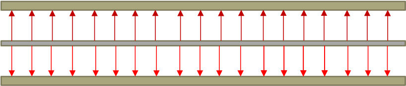
We are not aware of any definitive previous proposals of a physical setting described by the above model. However, we suggest that a thin magnetic metal beam suspended between two electromagnets as shown in Figure 1 could represent a reasonable physical system with the same properties as our PDE model, in the same way that the equation would reasonably correspond to a thin (very) flexible magnetic metal wire suspended between two electromagnets. Similar reasoning has been used with the well-known Duffing equation (ODE); in [9] the authors report on creating a realistic physical model of a flexible beam suspended between two magnets, which is compared favorably to the predicted theory; the potential function is the same as the one we use. Also, our interpretations are closely related to the classical interpretations of the linear wave equation () and the linear beam equation () as representing small vibrations of a flexible string and a beam respectively.
The nonlinear beam model (1) is similar to the model
| (2) |
which has been studied intensely both analytically and numerically over three decades now [10, 11]; see also the recent book [12] summarizing the current state of understanding for such Klein-Gordon models. Our aim in the present first work is to present some of the basic features of the biharmonic analogue of the model, which we will hereafter term biharmonic or B for short. In the present work, we first present numerical computations and simulations for a single kink at the level of both standing and traveling waves. Next, we study the behavior of kink-antikink solutions which is well-known to be particularly elaborate in the standard model [10, 11, 13, 14, 15, 16, 17]. The latter, per the recent work of [16, 17] (see also [12]) is still an ongoing research theme. Here, we show that the interactions between kink and antikink are in some ways much simpler, yet at the same time in other ways fundamentally more complex. The interactions up to speeds of the incoming wave of about are nearly elastic and, importantly, effectively repulsive, i.e., the kink and antikink never get to reach the same location while interacting. For large speeds between and the large kinetic energy of the coherent structures overcomes their interaction barrier and leads to collision and separation with the waves moving at speeds lower than the incoming ones. In between, a delicate trapping window arises with edges featuring a very complex (oscillatory and logarithmic) dependence of the outgoing vs. the incoming velocity. We present the relevant dependencies, for the first time to our knowledge, and expose some of the interesting questions arising from our numerical computations worthwhile to address in future studies.
2 Numerical Methods
In order to simulate Eq. (1) numerically we discretize the spatial domain on the interval with an increment of . We use a Fourier-based spectral differentiation matrix as in [18] to approximate as and to approximate as . This turns the PDE (1) into a system of ODE’s and we use Matlab’s built in ODE solver ode45 to simulate the kink and antikink evolution therein.
3 Single Kink Solutions
A kink solution for Eq. (1) (or for Eq. (2)) is a solution for which as respectively, as shown in Figure 2 in the first panel. An antikink is a solution for which as respectively; an antikink can be obtained from a kink by reflection about either the horizontal or vertical axis. In this section, we study the behavior of a single kink solution numerically. We start with the steady state solution, and study its existence and stability numerically. Next, we consider the moving single kink solutions, examining their corresponding properties. We also briefly touch upon energy and momentum conservation considerations indicating the corresponding properties of the models and examining them as a numerical check the validity of our direct simulations.
3.1 Steady state Kink Solutions
Steady state kink solutions of Eq. (1) satisfy
| (3) |
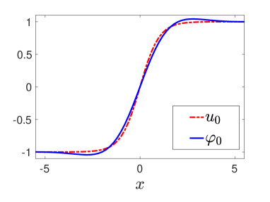
We numerically solve this fourth order BVP using Matlab’s fsolve and choose as initial guess the explicitly known solution to the steady-state model, namely, . The result of the corresponding computation is shown in the top left panel of Fig. 2.
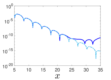
It is worthwhile to briefly consider the asymptotics of the relevant kink, i.e., how it approaches the homogeneous steady states . Substituting into Eq. 3, we obtain (as ) ; choosing the root , we get for small , where denotes a suitable constant. In Fig. 2, the top right panel shows the plots for and the fitted curve for the function in the form:
| (4) |
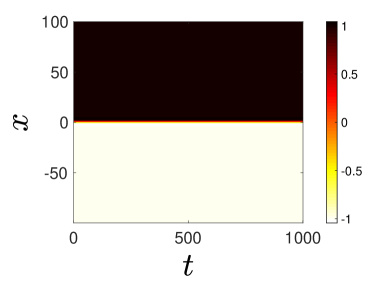
where and are parameters. We use Matlab’s lsqcurvefit function to find the values and 95% confidence intervals for and . The values and the intervals for those parameters are presented in Table 1. As seen in the Table, the numerically obtained intervals support the theory where and (the exponential spatial decay rate and the wavenumber of the spatial oscillation) are expected to be 1. Note that the fit in the top right panel of Fig. 2 is excellent with a divergence occurring at around due to the accuracy settings used in finding the numerical solution . The bottom panel of Fig. 2 illustrates the dynamical evolution of the relevant coherent structure predisposing us through its robust dynamical evolution for the spectral stability of the kink to which we now turn below.
| Parameters | Values | 95 % CI |
|---|---|---|
| a | 0.9998 | [0.9978, 1.0019] |
| b | 0.9650 | [0.9525, 0.9775] |
| c | 0.9998 | [0.9984, 1.0013] |
| d | 0.4086 | [0.4015, 0.4156] |
To study the stability of the steady state, we consider the linearization around the steady kink solution. Assume
| (5) |
where is the perturbation assumed to be small when . When we substitute Eq. (5) into Eq. (1), we get the linearized equation as
| (6) |
Defining , we can convert Eq. (6) into a first order linear system
| (7) |
where
| (8) |
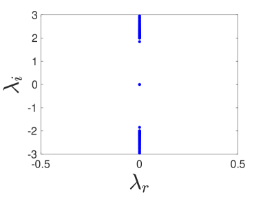
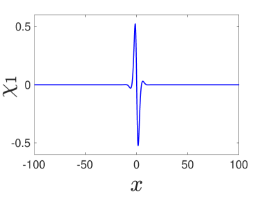
We solve the relevant spectral eigenvalue problem (of the operator ) numerically. In Fig. 3, we show the eigenvalues of this operator and the eigenfunction corresponding to the internal mode at . As seen in the figure, the purely imaginary nature of all the eigenvalues indicates that the steady state kink solution is spectrally stable. This is, indeed, in line with our numerical observations of Fig. 2.
3.2 Moving Single Kink Solutions
In this section, we examine the dynamical evolution of a single kink solution in the form: where is the speed. For second order differential equations like the model, we can apply a Lorentz transformation to the steady state kink solutions and obtain the moving ones. However, this is not the case for the B equation because it is a fourth order differential equation.
The equation that a traveling wave must satisfy can be found by assuming and substituting into Eq. (1) to get
| (9) |
where . Thus we solve Eq. (9) numerically in order to identify a numerically accurate traveling wave profile. We use (the known traveling wave solution at ) as an initial guess for in order to find the moving kink solutions.
For the stability of these solutions, we study the spectrum of the linearized operator about these moving solutions. Converting Eq. (1) to the new coordinates and (a moving coordinate system), we obtain
| (10) |
Steady-state solutions of Eq. (10) are traveling wave solutions of Eq. (1) and are given by Eq. (9). To determine stability we assume:
| (11) |
where is the perturbation around the traveling solution and assumed to be small. When we substitute Eq. (11) into Eq. (10) and use Eq. (9), as well as the approximation , the linearized equation is as follows:
| (12) |
Defining , Eq. (12) can be rewritten as a first order linear system of the form:
| (13) |
where
| (14) |
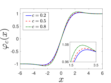
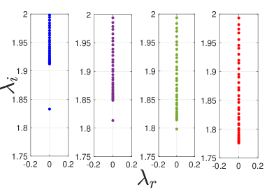
In Fig. 4, we show the numerical moving kink solutions for three values of and also present the spectra of the linearized operator around solutions of different speeds. Importantly, it can be seen that the relevant solutions are spectrally stable. Additionally, it can be observed that the first three panels feature an internal mode with a frequency outside of the continuous spectral band; however, the rightmost panel associated with speed shows no such mode indicating that apparently the relevant mode has disappeared inside the continuous spectrum.
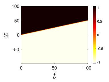
We have also examined the dynamics associated with the relevant traveling waves. As a prototypical example, by using the initial conditions:
| (15) |
we can simulate a moving single soliton moving with velocity where is the solution to Eq. (9). The bottom panel in Fig. 4 shows the contour plot of the moving kink traveling with the speed . The relevant solution appears to be robustly propagating for the time scales considered suggesting that the relevant traveling wave kink is a genuine stable traveling solution of the original problem of Eq. (1). We have indeed confirmed that similar results can be obtained for other speeds, in line with our theoretical analysis (data not shown here).
3.3 Conservation Laws and Numerical Method Validation
3.3.1 Conservation of Energy
It is known that the Eq. (1) has Hamiltonian structure, therefore it conserves an energy (Hamiltonian) functional given by
| (16) |
where the kinetic and potential energy contributions of the field, respectively, are
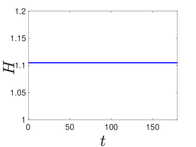
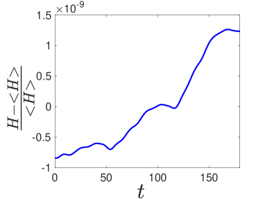
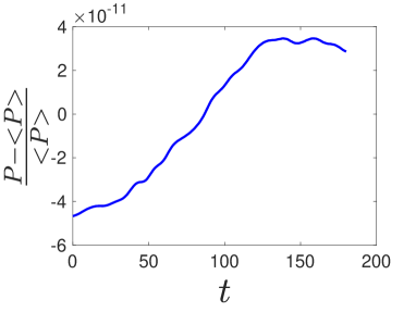
Since , is a given constant for a chosen initial field configuration. In our simulations, the average value of is of , while the deviations from the mean are (for the numerous examples we considered) no more than . In this way, we use energy conservation as a partial check of the validity of our numerical results. In Fig. 5, we show a moving single kink with the speed . The bottom left and bottom right panels show, respectively, the total energy and the deviation from the mean value (calculated over the time horizon of our entire numerical computation).
3.3.2 Conservation of Momentum
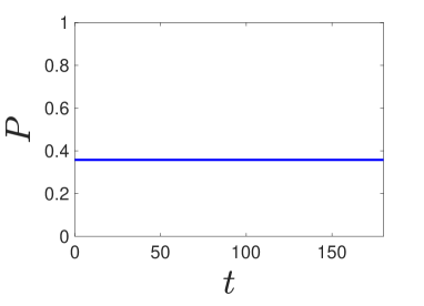
Similarly to the energy, another important conservation law of the B equation is that of the linear momentum (associated also with the invariance of the kink structures we discussed above with respect to translations). The momentum on the interval is defined as . Differentiating with respect to time , it is straightforward to infer that the relevant quantity is conserved. In Fig. 6, we show the total momentum and the deviation from the mean for a moving single kink with the speed . Once again the relevant quantity is of order unity, while the deviations from its mean value are of O indicating the accuracy of our numerical computations.
4 Kink-Antikink Collisions
Lastly, and most importantly for our study of the properties of the B model, we now turn our attention to the topic of kink-antikink solutions. Recall that such collisions have been the topic of intense scrutiny in the regular model [10, 11, 13, 14, 15, 16, 17]. Importantly, the recent work of [16, 17] and the summary of [12] suggest that the relevant topic is far from complete. Hence, this is naturally a theme of principal interest within the (fourth derivative) model discussed herein, namely the B equation.
For the separation half-distance we choose and let the kink and antikink approach each other at various velocities (), and then record the average velocity at which they separate after the interaction (). To generate initial conditions, we follow a technique that we developed in an earlier work [19]. In particular, we use Matlab’s lsqnonlin to find which minimizes the quantity (square of the -norm of the left side of Eq. (9)) subject to the additional constraints that the kink position remain at and the antikink at . This is necessary because Eq. (9), which applies to a traveling wave solution to Eq. (1), may not have a solution when a kink and antikink are involved (for a single kink or antikink a solution is always possible). Thus a least-squares approximation is the best one can do. In this way, we ensure that the initial conditions produce the “best” possible approximation to a B kink and antikink traveling towards each other, each with speed , and consequently produces the minimal possible radiation as a result of the coherent structure “superposition”.
As initializer to lsqnonlin, similar to [19], we use
where is the traveling wave solution to Eq. (2) at . Here, is the Heaviside unit-step function. Then the initial conditions that we use for moving kink-antikink system are:
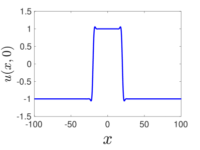
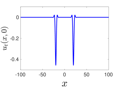
Note that without the “sign” function, the kink and antikink would move in the same direction. See Figure 7 for a typical initial position profile and initial velocity profile.
It is relevant to recall here the particularly complex phenomenology of the regular model. There, sufficiently large velocities (), the kink and antikink always inelastically scatter, while for sufficiently small ones () they always trap each other into a breathing, so-called bion, state. In between, a remarkable wealth of fractal in nature multi-bounce (2-bounce, at the edge of which there exist 3-bounce, at the end of which 4-bounce, and so on) windows arise. In these, the coherent structures, despite the (kinetic) energy loss they incur during the first collision, they manage to escape each other’s attraction via a resonance mechanism involving the kink’s internal mode after multiple (respectively, 2-, 3-, 4-) bounces.
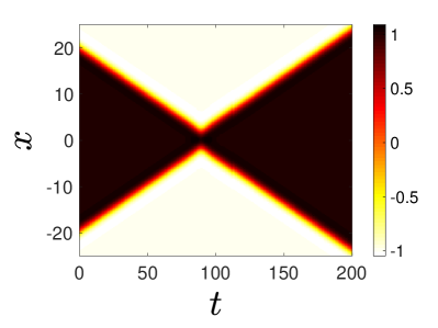
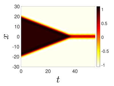
The collision picture in the B model turns out to be dramatically different and while in some ways it is quite simpler, in others it turns out to also be rather complex. More specifically, for most initial velocities used we end up with three cases. In the first case, where (the no bounce window), the kink and antikink move towards each other, but after some certain time they stop and move away from each other. In the second case where (the infinitely many bounce window) the kink and antikink move towards each other and collide, but they do not have enough kinetic energy to escape from each other. They end up with infinitely many collisions, i.e., trapping each other. In the third case, where (the one bounce window), the kink and antikink collide only once and they escape from each other forever as seen in Figure 8.
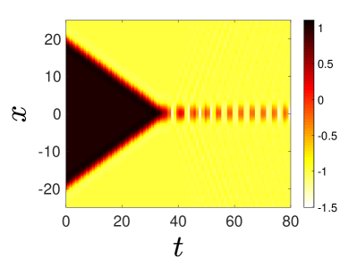
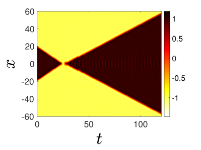
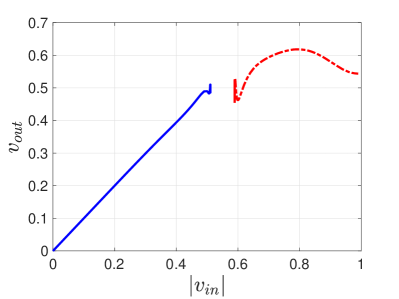
It is clear from the nature of the interaction of the top left panel of Fig. 8 that the kink and antikink effectively “repel” each other when they get sufficiently close. That is to say if they do not possess sufficiently large speed, they will not be able to overcome the energetic barrier that precludes them from colliding. In Fig. 9, we present the relation between and . We observe that for small values of , there is a linear relationship with , such that to a very good approximation = . We do not see a linear relation for larger values of . This suggests that small kinetic energies (smaller than the one of the energetic barrier precluding the kink-antikink collision) will lead to direct reflection with minimal conversion to a different form of energy. On the other hand, if the waves are incoming with sufficiently large speed, they will collide and separate after a single bounce (bottom panel of Fig. 8). However, in that case, as shown in Fig. 9, the outgoing speed will be significantly smaller than the incoming one signaling the conversion of the kinetic energy into internal energy and also importantly small amplitude dispersive radiation wavepackets.
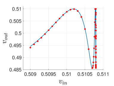
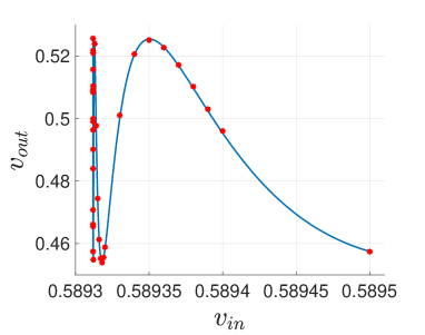
The most interesting case naturally lies between the two above limits. Here the initial kinetic energy of the waves is higher than the (repulsive) barrier, thus the structures will reach each other and collide. Our detailed numerical computations in the vicinity of the boundary of such a collision have revealed a surprising feature. This occurs near the boundaries of the infinitely-many bounce window. Letting represent the left boundary of the infinitely-many bounce window, and the right boundary of the same window, we see that there appear to be oscillations in the versus curve as approaches from the left and as approaches from the right. Closer inspection of these regions show that this is indeed the case.
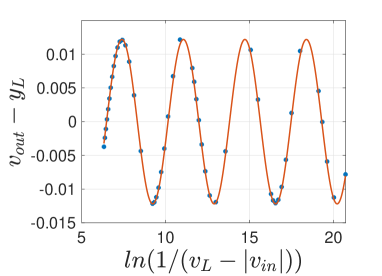
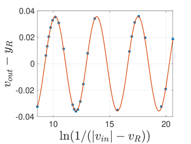
In Figure 10 we show close-up views of these two regions (top two panels). In both cases we observe oscillations that get more rapid as the critical point ( or ) is approached. Upon a systematic data exploration, it was found that the data follows a pattern similar to that of as . Thus it appears that no limit for exists as approaches from the left or from the right. This is in stark contrast to the corresponding model given in Eq. (2). For that model, we know that always goes to zero at the boundaries of any n-bounce window. The versus data near each critical point ( and ) was first translated to the origin (i.e., or was respectively subtracted), then , ( the translated ) was plotted against the translated data. The results are in the bottom two panels of Figure 10. Since the pattern of the data appears sinusoidal, a numerical fit to a sine function of the form was performed (with representing the transformed data). The results appear in the four panels of Figure 10. In the bottom two panels the transformed data and fitted functions appear, and in the top two panels the original data and the model for the data (derived from the fitted functions in the bottom panels). In all cases the models fit the data quite well ( or higher). This suggests a very delicate oscillatory regime of outgoing velocities both on the side of a of and on that of .
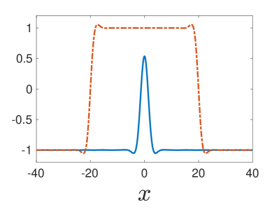
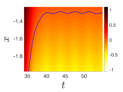
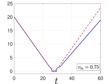
We end this section with a bit of a speculation about the source of these oscillations. While the regimes of individual behaviors of the B model are far fewer and more well defined than in the second derivative analogue, these oscillations are a source of unexpected complexity. In Figure 11 we show the results of using the initial conditions and (the dashed red curve shows the initial position in the first panel) that result in a kink-antikink pair approaching what appears to be a steady state (blue curve in first panel). The second panel is a contour plot showing that this apparent steady state develops at approximately and persists to at least . Near the other critical value of about 0.5896, we also observe that the kink-antikink solitions appear to reach a steady-state for some time (in a similar manner, hence omitted here). In fact, the combined kink-antikink state is oscillating slightly about the steady state shown in the left panel which can be seen in an enlargement of the contour plot in the region , shown in the lower panel in Figure 11. Thus for very small changes in near the critical values (but not entering the range between the two critical values), the oscillating solitons will separate at different points in their oscillatory cycles, resulting in the different (oscillating) outgoing velocities .
Finally we note that with very small perturbations in which do enter the region between the critical values, we observe that after the kink-antikink pair undergoes small oscillations about a steady state for a while, they get stuck with infinitely many collisions (bion state). This suggests that in addition to the potential barrier discussed above, there exists also a bound state in the form of a potential well that can trap the multi-kink dynamics. The oscillatory structure of the outgoing velocities outside the region between the critical values is indicative of the possibility that multiple such equilibrium states (saddles and centers) may exist. Exploring the structure and stability of these steady states (as dictated by the oscillatory nature of the kink tails) will be a subject of future work.
4.1 Collective Coordinates Method (ODE)
One of the prototypical methods that have been used to attempt to understand the dynamics of the model is the collective coordinate (CC) method. Here, the evolution of the kink and antikink is represented by a suitable superposition ansatz featuring a finite number of time-dependent collective variables (such as the center and width of the kinks or the amplitude of their internal mode) and the evolution of the ODEs for these variables is developed (typically) based on the underlying Lagrangian of the PDE model. In this setting the original analysis of [20] was used later, e.g., by [13] and further in a quantitative fashion in [14, 15]. However, recently, the work of [16, 17] revealed some inconsistencies in the original ODE derivation of [20] leading to the need for reconsideration of the entire CC framework for the model.
Here, our scope is more modest, as we will only illustrate how to consider the setting with a single collective coordinate, namely the center of the kink and antikink. As we will discuss further below, while partially useful in the B model, this approach has nontrivial limitations that are worthwhile to further explore and amend in future studies. Our aim is to reduce the full PDE with infinitely many degrees of freedom to a simple model with only one degree of freedom and explore the potential successes and the nontrivial limitations of such an approximation.
Assuming that we characterize the kink-antikink motion by utilizing the ansatz
| (17) |
where is the steady state kink solution of Eq. (1) whose center is located at and is the steady state antikink solution whose center is located at . Note that the steady state solution centered at , i.e. is shown in Fig. 2. Our aim is to study the behavior of with the initial conditions and where is the distance from the origin, and is the initial speed of the kink. Using the Lagrangian of the PDE model in the form:
| (18) | ||||
we substitute the ansatz of Eq. (17) to obtain:
| (19) | ||||
Here
| (20) | ||||
By applying the Euler-Lagrange prescription
| (21) |
we obtain the dynamical evolution:
| (22) | ||||
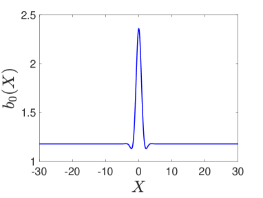
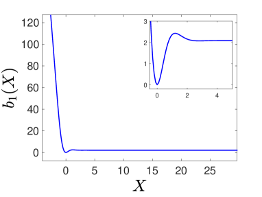
We solve these equations numerically by using the initial conditions and . We numerically compute the integrals on the interval . We use MATLAB’s built-in fourth-order Runge–Kutta variable-step size solver ode45 with built-in error control. In Fig. 12, we show the coefficient functions and .
4.1.1 Results
The CC method gives a very good match with the PDE results when is small, that is when . We observe a difference when we start increasing . This difference gets bigger as gets closer to . The relevant deviation becomes maximal when there is an infinite bounce window in the B PDE simulations. It is important to appreciate that the CC method cannot capture those bounces. Bearing a single degree of freedom (dof) and given the conservation of energy, the CC method can at best capture a pair of kinks that interact and become outgoing ones with the same speed as they were incoming. Hence, beyond this threshold where the phenomenology deviates from this symmetric scenario, the reduction of the PDE to the 1-dof manifold is one that is too restrictive to capture the relevant dynamics. For bigger values of , we only see a good match until the kink and antikink collide. After the collision, in the CC method, as described above, the kinks separate from each other with a speed practically equal to whereas in the PDE the kinks separate from each other with a speed that is smaller than . This inelasticity of the collision is due to the additional dof’s of the B field theory which are naturally not captured in this reduced CC formulation.
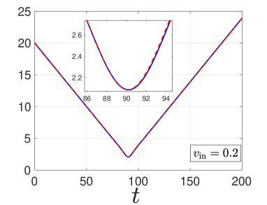
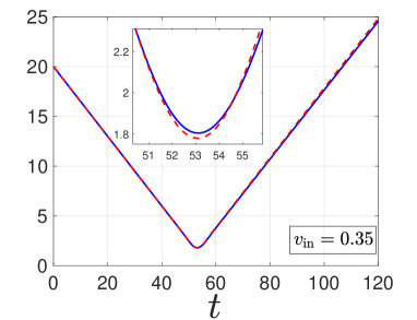
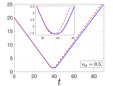
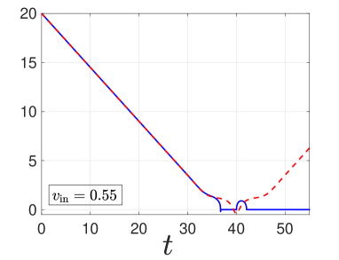
In Figure 13, we plot the PDE and the ODE solutions (obtained using CC method) for various values of . The PDE plot in the figure is the position of the approximate center of the antikink solution as defined by its intersection with the x-axis. As seen in the figure, we get a nearly perfect match for . When we increase to , we see a slight difference. That difference gets more noticeable when is . When we take , we see a divergence after the collision. For , we only see a good match until the collision.
5 Conclusions and Future Work
In the present work we have explored the biharmonic (B) model and some of the central properties of its kink solutions. We have illustrated that the model has kinks with tails that are distinctly different than those of the standard model in that they bear an oscillatory structure (instead of the monotonic kinks in ). We have also performed a spectral analysis of both static and traveling kinks. The case of the latter is not as straightforwardly mappable to the former in the B model due to the absence of the Lorentz invariance. Both static kinks and traveling ones below a certain speed appear to have an internal mode in the B model. Lastly, we tackled collisions between a kink and an antikink. These were found to be quite different than the complex fractal collision structure of the regular model. Here, the scenarios turned out to be far more clear in their structure with elastic apparent repulsion between the wave occurring at small speeds, collision into an infinite bounce capture for a short range of intermediate ones and eventually inelastic single bounces at large speeds. Nevertheless, a different source of complexity was unveiled in the two transition regions between these three regimes. Namely, a delicate oscillatory logarithmic dependence of the outgoing vs. incoming velocity was revealed that was intuitively attributed to the more complex tail and associated interaction structure of the two waves, but which also merits further elaboration in future work.
Lastly, we attempted the most simple version of the CC method towards characterizing the B model kink-antikink collisions. The CC method we have applied has only one degree of freedom, so it is expected not to fully capture the PDE behavior. It is natural to expand this by attempting to take into consideration the internal mode of the kink and antikink. Then, the corresponding ansatz that is relevant to consider becomes:
| (23) |
where which is the time-dependent displacement of the kink from the origin and is the amplitude of the internal mode perturbation and is the eigenfunction corresponding to the lowest (positive) eigenfrequency of the kink. A question that arises, however, in this setting is which frequency it is suitable to consider, as the static and traveling kink are not effectively equivalent and there is a dependence of the internal mode frequency on the corresponding speed. Using, as is done in the frequency of the static kink and attempting to solve the corresponding ODE system, one obtains a numerical instability around . This has been a common issue with -models, as discussed, e.g., in the recent review of [12]: it has been dubbed the null-vector problem [21]. Reduced ODE systems were studied in the earlier works assuming the terms with higher order derivatives of and stayed negligible. Our numerical computations suggest that this is not a suitable assumption around . Hence, clearly there are some important challenges ahead, especially as regards an understanding of the phenomenology of collisions and, more generally, of kink-antikink interactions and “bound states”. These appear to us to certainly be worthwhile to consider in future studies and will accordingly be reported in future publications.
References
- [1] S. Levandosky, Stability and instability of fourth order solitary waves, J. Dynam. Differential Equations, 10, 151 (1998).
- [2] A.R. Champneys, P.J. McKenna and P.A. Zegeling, Solitary waves in nonlinear beam equations: stability, fission and fusion, Nonlinear Dynamics, 21, 31 (2000).
- [3] Y. Chen, P.J. McKenna, Traveling waves in a nonlinearly suspended beam: theoretical results and numerical observations, J. Differential Equations, 136, 325 -355 (1997).
- [4] P. Karageorgis, P. J. McKenna, The existence of ground states for fourth-order wave equations, Nonlinear Anal., 73, 367 (2010).
- [5] A. Blanco-Redondo, C. Martijn de Sterke, J.E. Sipe, T.F. Krauss, B.J. Eggleton and C. Husko Pure-quartic solitons, Nature Comms. 7, 10427 (2016).
- [6] I. Posukhovskyi and A. Stefanov, On the normalized ground states for the Kawahara equation and a fourth order NLS, arXiv:1711.00367.
- [7] M.J. Ablowitz, Nonlinear Dispersive Waves, Cambridge University Press (Cambridge, 2011).
- [8] A. Demirkaya, M. Stanislavova, Numerical results on existence and stability of standing and traveling waves for the fourth order beam equation, Discrete Contin. Dyn. Syst.-B, 24, 197 (2019).
- [9] F. C. Moon and P. J. Holmes, A magnetoelastic strange attractor, Journal of Sound and Vibration, 65, 275 (1979).
- [10] D. K. Campbell, J. S. Schonfeld, and C. A. Wingate, Resonance structure in kink-antikink interactions in theory, Phys. D, 9, 1 (1983).
- [11] T.I. Belova and A.E. Kudryavtsev, Solitons and their interactions in classical field theory, Phys. Usp., 40, 359 (1997).
- [12] P.G. Kevrekidis, J. Cuevas-Maraver (Eds.), A Dynamical Perspective on the model, Springer-Verlag (Heidelberg, 2019).
- [13] P. Anninos, S. Oliveira, and R.A. Matzner, Fractal structure in the scalar theory, Phys. Rev. D, 44, 1147 (1991).
- [14] R.H. Goodman, R. Haberman, Kink-antikink collisions in the phi-four equation: The n-bounce resonance and the separatrix map, SIAM J. Appl. Dyn. Sys., 4, 1105 (2005).
- [15] R.H. Goodman, Chaotic scattering in solitary wave interactions: A singular iterated-map description, Chaos, 18, 023113 (2008).
- [16] H. Weigel, Kink–antikink scattering in and models, J. Phys. Conf. Ser., 482, 012045 (2014), arXiv:1309.6607.
- [17] I. Takyi and H. Weigel, Collective coordinates in one-dimensional soliton models revisited, Phys. Rev. D, 94, 085008 (2016), arXiv:1609.06833.
- [18] L. N. Trefethen, Spectral Methods in MATLAB, SIAM (Philadelphia, 2000).
- [19] I. C. Christov, R. Decker, A. Demirkaya, P. G. Kevrekidis, V. A. Gani, Long range interactions, Phys. Rev. D, 99, 016010, (2019).
- [20] T. Sugiyama, Kink-antikink collisions in the two-dimensional model, Prog. Theor. Phys., 61, 1550 (1979).
- [21] J.G. Caputo and N. Flytzanis, Kink-antikink collisions in sine-Gordon and models: Problems in the variational approach, Phys. Rev. A, 44, 6219 (1991).