Localization with overlap fermions

Abstract

We study the finite temperature localization transition in the spectrum of the overlap Dirac operator. Simulating the quenched approximation of QCD, we calculate the mobility edge, separating localized and delocalized modes in the spectrum. We do this at several temperatures just above the deconfining transition and by extrapolation we determine the temperature where the mobility edge vanishes and localized modes completely disappear from the spectrum. We find that this temperature, where even the lowest Dirac eigenmodes become delocalized, coincides with the critical temperature of the deconfining transition. This result, together with our previously obtained similar findings for staggered fermions shows that quark localization at the deconfining temperature is independent of the fermion discretization, suggesting that deconfinement and localization of the lowest Dirac eigenmodes are closely related phenomena.

I Introduction

Strongly interacting matter is known to undergo a crossover at high temperature. In the low temperature regime quarks are bound together to form hadrons due to color confinement. During the crossover the boundaries of the hadrons become blurred and matter goes into the state of quark-gluon plasma (QGP). At the same time the spontaneously broken chiral symmetry becomes approximately restored. Besides deconfinement and chiral restoration, there is a third phenomenon that happens in the crossover region. Above the crossover temperature the lowest lying eigenmodes of the Dirac operator become spatially localized Halasz:1995vd -Giordano:2014qna . This is in sharp contrast to the temperature regime below the crossover, where all the quark eigenmodes are extended Verbaarschot:2000dy .

In the high temperature phase the spectrum of the Dirac operator can be separated into two regions. At the low end of the spectrum there are only localized eigenmodes and their eigenvalues can be described by Poisson statistics. In the upper part of the spectrum the eigenmodes are extended and the corresponding eigenvalues obey Wigner-Dyson statistics Verbaarschot:2000dy . At fixed temperature this transition in the spectrum between the localized and extended eigenmodes was shown to be a genuine second order transition, and its correlation length critical exponent was found to be compatible with that of the Anderson model in the same symmetry class Giordano:2013taa . Building on this analogy with Anderson transitions, we call the critical point separating the localized and extended modes in the spectrum, the mobility edge, $\lambda_{c}$ mobility . While in the Anderson model the mobility edge is controlled by the amount of disorder in the system, in QCD an analogous role is played by the physical temperature. As the temperature is lowered towards the crossover, the mobility edge moves down in the spectrum, the part of the spectrum corresponding to localized eigenmodes occupies a narrower and narrower band in the spectrum around zero. Eventually, at a well defined temperature that we denote by $T_{c}^{loc}$, the mobility edge vanishes, implying that even the lowest Dirac eigenmodes become delocalized.

In QCD with physical quark masses the critical temperature of the localization transition, $T_{c}^{loc}$ is in the crossover region Giordano:2014qna . This raises the question whether this is just a coincidence or there is some deeper physical connection between the localization transition and the chiral and/or the deconfinement transition. A possible way to test this is to move in the parameter space of QCD to a regime where there is a genuine finite temperature phase transition and check whether its critical temperature coincides with $T_{c}^{loc}$. The simplest way to do that is to consider the limit of infinitely heavy quarks, i.e. the quenched approximation to QCD, which is known to have a first order deconfining phase transition at a temperature of around $300$ MeV.

The possibility of linking the QCD transition to an Anderson-type localization transition in the Dirac spectrum was first raised more than ten years ago by Garcia-Garcia and Osborn. They studied the spectral statistics of the Dirac operator in an instanton liquid model GarciaGarcia:2005vj and in quenched as well as full lattice QCD GarciaGarcia:2006gr and found evidence that around the chiral transition the spectral statistics of the Dirac spectrum changes from Wigner-Dyson towards Poisson. This indicates that the chiral transition is accompanied by a localization transition for the lowest eigenmodes of the Dirac operator, however, at that time no no attempt was made at a determination of $T_{c}^{loc}$, the critical temperature of the localization transition, with a precision comparable to how $T_{c}$, the critical temperature of the quenched deconfining phase transition is available in the literature.

In a previous paper we explored this possibility by studying the spectrum of the staggered quark Dirac operator in quenched gauge field backgrounds, generated just above the finite temperature phase transition Kovacs:2017uiz . For staggered fermions we calculated $T^{loc}_{c}$, the critical temperature of the localization transition and found that it coincided with that of the deconfining transition. Our results, obtained on lattices with three different temporal extensions, $L_{t}=4,6$ and 8, suggest that the agreement of the localization and the deconfining transition temperature is universal and is very likely to hold in the continuum limit, provided the staggered discretization of quarks is in the correct universality class also for the localization transition.

Unfortunately, staggered quarks are not in the same random matrix theory symmetry class as continuum quarks Verbaarschot:2000dy . Moreover, their chiral symmetry is also different from that of continuum quarks. Although the staggered Dirac operator is expected to have the correct continuum limit, it is still possible that at finite lattice spacing it does not properly describe some properties of the lowest quark eigenmodes, the ones that are our main concern here for studying the localization transition. This is a potentially important issue, as the lowest part of the Dirac spectrum is particularly sensitive to the chiral properties of the given discretization. Therefore, in the present work we chose to repeat our previous staggered study with the overlap Dirac operator that has exact chiral symmetry already for finite values of the lattice spacing Narayanan:1993ss .

Besides this, there are two more reasons concerning localization, why it is important to verify our previous results with the overlap. Firstly, overlap fermions with the $SU(3)$ gauge group are in the same random matrix symmetry class, the chiral unitary class, as fermions in the continuum. Secondly, unlike the staggered action that is ultralocal, the overlap action couples quark degrees of freedom to arbitrarily large distances, albeit with couplings falling exponentially with the distance. Since in the theory of Anderson-type models localization is generally known to strongly depend on the range of the couplings (hopping terms in the Hamiltonian) Evers:2008zz , it is interesting to check whether the non-locality of the overlap Dirac operator has any influence on the localization transition in QCD. In fact, to our knowledge, this is the first study where the mobility edge is explicitly determined in QCD with chiral quarks.

In the present work we used a subset of the gauge configurations that were previously generated for our earlier staggered study. Since overlap spectra are significantly more expensive to calculate than staggered spectra, here we limited our study to one value of the temporal lattice size, $L_{t}=6$. We computed the mobility edge for gauge ensembles generated with six different values of the gauge coupling, $\beta$, all corresponding to temperatures slightly above the deconfining transition. By extrapolation we determined the gauge coupling $\beta_{c}^{loc}$ where the mobility edge vanished and all localized eigenmodes disappeared from the Dirac spectrum. Confirming our previous staggered result, we found $\beta_{c}^{loc}$ to be compatible with the critical gauge coupling of the deconfining phase transition for $L_{t}=6$.

The plan of the paper is as follows. In Sec. II we describe the lattice ensembles used for the calculation and show how we computed the mobility edge from the Dirac spectra. In Sec. III we discuss the determination of the critical coupling of the localization transition. In Sec. IV we draw our conclusions and finally in the Appendix we describe the technical details of the unfolding of the spectrum.

II Calculation of the mobility edge

The Dirac operator that we used for this study was the overlap with Wilson kernel parameter $M=-1.3$. As smearing of the gauge field is known to improve some properties of the overlap and also makes the calculations faster Kovacs:2002nz , two steps of hex smearing Capitani:2006ni were applied to the gauge field before inserting it into the overlap. The gauge field configurations we used here were quenched Wilson action lattices with temporal extension $L_{t}=6$. In Table 1 we collected the parameters of the simulations.

$\beta$	$L_{s}$	$N_{c}$	$N_{evs}$
5.91	40	741	80
5.92	40	821	80
	32	3823	50
	24	4668	25
5.93	40	750	80
5.94	40	856	80
5.95	40	835	80
5.96	40	609	80
	24	3915	25

Table 1: Simulation parameters (from left to right): the Wilson plaquette gauge coupling, the size of the lattice in the spatial direction, the number of configurations and the number of eigenvalues computed for each configuration. All the lattices had a temporal extension of $L_{t}=6$.

On each gauge configuration we computed a number of lowest eigenvalues of $D^{\dagger}D$, where $D$ is the overlap Dirac operator. In what follows we always work with the eigenvalues of $D^{\dagger}D$ that are the magnitude squared of the corresponding eigenvalues of the Dirac operator $D$. Since our analysis is based on the unfolded spectrum, which is invariant with respect to monotonic reparametrizations of the spectrum, it makes no difference that we perform the analysis in terms of the eigenvalues of $D^{\dagger}D$. As explained in the Appendix, we take extra care to make even the assignment of eigenvalue pairs to spectral windows to be reparametrization invariant. To make the notation simpler and avoid having to write the absolute value squared everywhere, we denote by $\lambda$ the eigenvalues of $D^{\dagger}D$, in terms of which we perform the entire analysis.

The number of eigenvalues to be computed per configuration was chosen to include all the eigenvalues to a point well above the mobility edge, $\lambda_{c}$. Having exact chiral symmetry, the overlap possesses exact zero eigenvalues in gauge field backgrounds with non-zero topological charge. Since these eigenvalues are all exactly at the lower edge of the spectrum, they do not contain any information relevant to the present study, we simply removed them from the spectra before further analysis.

Localized and delocalized eigenmodes are characterized by different statistics of the corresponding eigenvalues. To track the transition throughout the spectrum and locate the mobility edge, we used the simplest spectral statistics, the unfolded level spacing distribution (ULSD), calculated locally, within narrow spectral windows of the spectrum. Unfolding, a transformation well known in the theory of random matrices, is a monotonic mapping of the spectrum that sets the local spectral density to unity everywhere throughout the spectrum. In particular, by construction, the unfolded eigenvalues are dimensionless and their average level spacing is unity. More details on how the unfolding was done are presented in the Appendix.

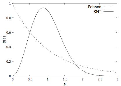
Unfolding is useful since both for localized and delocalized eigenmodes, universally valid analytic results are known for the ULSD of the corresponding eigenvalues Verbaarschot:2000dy . Spectra corresponding to localized eigenmodes obey Poisson statistics and the ULSD follow the exponential distribution,

$$p(s)=\exp(-s),$$ (1)

where $s$ is the level spacing between the nearest neighbor unfolded eigenvalues.

In the case of extended modes the ULSD is also known analytically, however, it is much more complicated than in the localized case and also depends on the random matrix symmetry class of the given model. A very good approximation to the ULSD in this case is provided by the so called Wigner surmise that for the unitary symmetry class, to which the overlap operator belongs, reads as

$$p(s)=\frac{32}{\pi^{2}}s^{2}\exp(-\frac{4}{\pi}s^{2}).$$ (2)

Notice that both the exponential and the Wigner surmise distribution are universal in the sense that they are free of any adjustable parameters. In particular, the originally dimensionful parameter, the local spectral density has been removed from the spectrum by the unfolding. For further reference we plotted the two distributions in Fig. 1.

Figure 1: The probability density functions of the level spacings in the cases when the eigenvalues obey the Poisson statistics (exponential distribution, dashed line) and Wigner-Dyson statistics (continuous line, Wigner surmise).

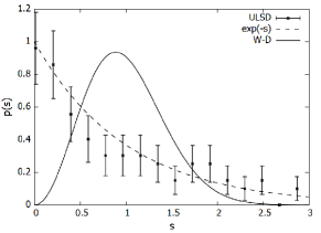
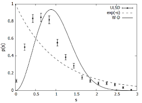
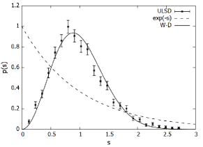
Our aim here is to scan the spectrum starting from zero and follow how the local ULSD changes from the exponential distribution of Eq. (1) to the Wigner surmise of Eq. (2). To this end we divide the spectrum into narrow spectral windows, compute the ULSD separately in each spectral window and follow how it changes throughout the spectrum. In Fig. (2) we show how the unfolded level spacing distribution evolve as the spectrum is scanned starting from the lowest eigenvalues (top panel) crossing the critical, transition region (middle panel) and finally moving up to the Wigner-Dyson regime (bottom panel).

Figure 2: The unfolded level spacing distribution in three different spectral windows for the $\beta=5.95$, $L_{s}=40$ ensemble. The spectrum is scanned from the lowest eigenvalues (top panel) with Poisson statistics, through the critical region (middle panel), up to the regime with Wigner-Dyson statistics (bottom panel). We also show the expected limiting distributions, the exponential (dashed line) and the Wigner surmise (continuous line).

However, monitoring the continuous change of a function (here the probability density of the unfolded level spacings) is complicated. To make this task easier, we choose a single parameter of this distribution and monitor how that changes throughout the spectrum. A simple choice for this parameter is the integral

$$I_{s_{0}}=\int_{0}^{s_{0}}p(s)ds$$ (3)

of the probability density up to the lowest crossing point $s_{0}\approx 0.508$ of the two limiting distributions, the exponential and the Wigner surmise. This choice of $s_{0}$ has the advantage that it maximizes the difference of the integral between the two limiting cases and thereby facilitates their clear separation.

Figure 3: The integrated probability density (defined in Eq. 3) as a function of eigenvalues $\lambda$ of $D^{\dagger}D$. The figure shows the data for $\beta=5.95$ with a spatial volume of $40^{3}$. The two short horizontal lines in the top left and the bottom right corner of the figure indicate the limiting values of $I_{s_{0}}$ for the Poisson (localized) and the Wigner-Dyson (delocalized) statistics.

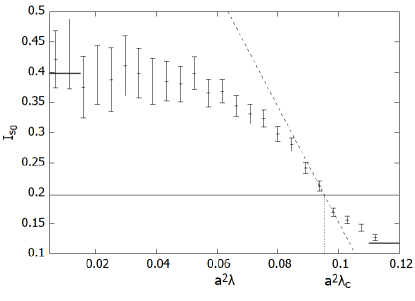
An example of how $I_{s_{0}}$ changes through the spectrum is shown in Fig. 3. As expected and can also be seen in the figure, in a finite volume $I_{s_{0}}$ changes smoothly from the value $I_{s_{0}}^{P}\approx 0.398$ corresponding to the exponential distribution to $I_{s_{0}}^{W}\approx 0.117$ corresponding to the Wigner surmise. However, based on the finite size scaling study of Ref. Giordano:2013taa , in the thermodynamic limit we expect the transition to become singular, as in a second order phase transition. The mobility edge, $\lambda_{c}$ that we eventually want to locate is this sharply defined singular transition point appearing only in the infinite volume limit. In a finite volume the definition of the “critical point” is somewhat arbitrary, however, a good choice is the point in the spectrum where $I_{s_{0}}$ is equal to the value $I_{s_{0}}^{crit}=0.1966$, corresponding to the critical distribution, known from the finite size scaling study of Ref. Giordano:2013taa . From now on, with a slight abuse of notation, we will call the point in the spectrum, $\lambda_{c}$, for which $I_{s_{0}}(\lambda_{c})=I_{s_{0}}^{crit}$, the mobility edge.

The quantity $\lambda_{c}$, defined in this way, can still have a volume dependence, but it is a good approximation to the mobility edge in the thermodynamic limit. To keep the finite size corrections under control, we calculated $\lambda_{c}$ on lattices of spatial linear size $L_{s}=24,32,40$. While the results on the smallest volume differed significantly from those on the other volumes, the results from the larger two volumes agreed within the statistical uncertainties. Therefore, for the rest of the analysis we always used the data from the largest volume, $L_{s}=40$.

Since the function $I_{s_{0}}(\lambda)$ has an inflection point at $\lambda_{c}$, around this point it can be well approximated with a straight line. We could thus easily determine $\lambda_{c}$ by solving the equation $I_{s_{0}}(\lambda_{c})=I_{s_{0}}^{crit}$ by approximating the function $I_{s_{0}}(\lambda)$ with a linear fit to the data in the given range (see Fig. 3).

III The critical temperature of the localization transition

So far we have shown how to calculate the mobility edge, $\lambda_{c}$, at a given temperature. Our final goal is to determine the temperature where the mobility edge vanishes and localized modes completely disappear from the Dirac spectrum. Since we keep the temporal size of the lattice fixed, the temperature can be controlled by the gauge coupling, $\beta$. We computed $\lambda_{c}$ for lattice ensembles generated at several different values of the gauge coupling, above, but close to the deconfining phase transition. The results are shown in Fig. 4. The range of couplings we used were limited by two factors. Firstly, even though the deconfining transition is of first order, the correlation length increases substantially towards the transition which puts a lower limit to the couplings for which finite size corrections can be kept under control. Secondly, we would like to extrapolate the function $\lambda_{c}(\beta)$ to find where it vanishes, and for the extrapolation only points close enough to the zero of this function are useful. Since we expected the zero of the function $\lambda_{c}(\beta)$ to be close to the deconfining transition, $\beta_{c}$, we limited our simulations to couplings not too far from this point.

Figure 4: The mobility edge as the function of the gauge coupling, approximated with a power function.

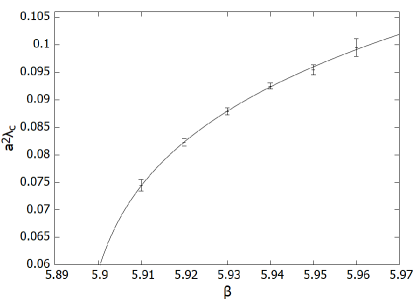
Finally, for the extrapolation we used the ansatz

$$\lambda_{c}(\beta)=p_{1}(\beta-\beta_{c}^{loc})^{p_{2}},$$ (4)

and its parameters $p_{1},p_{2}$ and $\beta_{c}^{loc}$ were fitted to the data. The ansatz turned out to describe the data remarkably well and using all six data points the resulting $\chi^{2}$ per degree of freedom was $\chi^{2}=0.67$. The fit along with the data is shown in Fig. 4. The resulting location of the localization transition is $\beta_{c}^{loc}=5.893(7)$, where we quoted the statistical uncertainty. Within the uncertainties this agrees with the critical point of the deconfining transition, $\beta_{c}=5.8943(3)$ Francis:2015lha . This, together with similar results obtained in Ref. Kovacs:2017uiz with staggered fermions, strongly suggest that independently of the fermion discretization, the localization transition and deconfinement happen at the same temperature, therefore the two phenomena are very likely to be strongly related.

IV Conclusions

We examined the localization transition of the quarks using the quenched approximation. We computed the lowest lying eigenvalues of the overlap Dirac operator above the critical coupling of the deconfining transition. By calculating the mobility edge, $\lambda_{c}$, for different gauge couplings we determined the function $\lambda_{c}(\beta)$ and extrapolated it to locate $\beta_{c}^{loc}$, where the mobility edge vanishes and all the eigenmodes become delocalized. We compared our result with the critical coupling of the deconfining phase transition and found that the two critical couplings are compatible; the localization transition and deconfinement occur at the same temperature. This is in agreement with our previous similar results with staggered fermions and indicates that localization and deconfinement are strongly related phenomena.

The present work was motivated by the fact that in QCD with physical dynamical quarks the localization transition occurs in the crossover region. On the one hand, our results clearly indicate that the localization transition is strongly related to deconfinement, which – at least on a qualitative level – probably carries over from the quenched model to real physical QCD. On the other hand, the quenched model cannot properly account for the other important transition, the chiral transition that also occurs in the QCD crossover. To see how localization is related to chiral restoration, it would be interesting to consider the other limiting case, the chiral limit. For massless light quarks, the chiral transition is expected to become a genuine phase transition Pisarski:1983ms and it could be tested whether its critical temperature agrees with the critical temperature of the localization transition. Although simulations in the chiral limit are technically immensely challenging, such a study could also provide additional insight into the physics of the restoration of chiral symmetry, how that happens in the massless (chiral) limit. Several questions related to this are currently under active study Ding:2019prx .

*

Appendix A Unfolding

Unfolding is a monotonic mapping of the eigenvalues that - by definition - renders the spectral density unity throughout the unfolded spectrum. This transformation is useful since it removes the scale, specific to the given spectrum and reveals universal spectral fluctuations. In principle unfolding can be done in several different ways, all equivalent for a dense enough spectrum. Here we did the unfolding by taking all the eigenvalues from all the configurations of the given ensemble and putting them into ascending order according to their magnitudes. To each eigenvalue we assigned its rank divided by the number of configurations, $N_{c}$, we used this mapping to define the unfolded spectrum. In this way the level spacing between successive unfolded eigenvalues is exactly $1/N_{c}$, which means that there are $N_{c}$ eigenvalues in an interval of unit length anywhere in the unfolded spectrum. This implies that the average spectral density per configuration is unity throughout the unfolded spectrum.

In the present work we used the unfolded level spacing distribution (ULSD) calculated from the spectrum unfolded in the above described way. In particular, we followed how the ULSD changed throughout the spectrum, starting from the Poisson statistics and going over to Wigner-Dyson statistics. This required the calculation of the local ULSD at different locations in the spectrum. In order to do this, we divided the spectrum into small spectral windows and calculated the ULSD in each window separately.

In principle, this method is straightforward, if the spectrum is infinitely dense. However, for finite density, there is an ambiguity in how we decide whether a pair of neighboring eigenvalues belongs to the given spectral window or not. We could demand that both members of the pair be within the spectral window in question. However, this would artificially limit the largest possible level spacings, especially for eigenvalues close to the edge of a spectral window. To avoid this uncontrolled truncation of the tail of the ULSD we chose the criterion that a pair of nearest neighbor eigenvalues was considered to belong to the given spectral window if the midpoint of the pair was in the window. To ensure that our procedure, including the assignment of pairs to spectral windows, is invariant with respect to monotonic reparametrizations of the spectrum, we applied the midpoint rule in the unfolded spectrum. This is easily done by mapping the endpoints of the spectral window into the unfolded spectrum. Notice, however, that we can and do still plot the results in terms of the original (not the unfolded) spectrum, as seen in Fig. 3.

References

- (1) A. M. Halasz and J. J. M. Verbaarschot, Phys. Rev. Lett. 74, 3920 (1995) doi:10.1103/PhysRevLett.74.3920 [hep-lat/9501025].
- (2) A. M. Garcia-Garcia and J. C. Osborn, Phys. Rev. D 75, 034503 (2007) doi:10.1103/PhysRevD.75.034503 [hep-lat/0611019].
- (3) A. M. Garcia-Garcia and J. C. Osborn, Nucl. Phys. A 770, 141 (2006) doi:10.1016/j.nuclphysa.2006.02.011 [hep-lat/0512025].
- (4) M. Giordano, T. G. Kovacs and F. Pittler, Int. J. Mod. Phys. A 29, no. 25, 1445005 (2014) doi:10.1142/S0217751X14450055 [arXiv:1409.5210 [hep-lat]].
- (5) J. J. M. Verbaarschot and T. Wettig, Ann. Rev. Nucl. Part. Sci. 50, 343 (2000) doi:10.1146/annurev.nucl.50.1.343 [hep-ph/0003017].
- (6) M. Giordano, T. G. Kovacs and F. Pittler, Phys. Rev. Lett. 112, no. 10, 102002 (2014) doi:10.1103/PhysRevLett.112.102002 [arXiv:1312.1179 [hep-lat]].
- (7) T. G. Kovacs and F. Pittler, Phys. Rev. D 86, 114515 (2012) doi:10.1103/PhysRevD.86.114515 [arXiv:1208.3475 [hep-lat]].
- (8) T. G. Kovacs and R. A. Vig, Phys. Rev. D 97, no. 1, 014502 (2018) doi:10.1103/PhysRevD.97.014502 [arXiv:1706.03562 [hep-lat]].
- (9) T. G. Kovacs, Phys. Rev. D 67, 094501 (2003) doi:10.1103/PhysRevD.67.094501 [hep-lat/0209125].
- (10) R. Narayanan and H. Neuberger, Phys. Rev. Lett. 71, no. 20, 3251 (1993) doi:10.1103/PhysRevLett.71.3251 [hep-lat/9308011]; R. Narayanan and H. Neuberger, Nucl. Phys. B 443, 305 (1995) doi:10.1016/0550-3213(95)00111-5 [hep-th/9411108].
- (11) F. Evers and A. D. Mirlin, Rev. Mod. Phys. 80, 1355 (2008) doi:10.1103/RevModPhys.80.1355 [arXiv:0707.4378 [cond-mat.mes-hall]].
- (12) S. Capitani, S. Durr and C. Hoelbling, JHEP 0611, 028 (2006) doi:10.1088/1126-6708/2006/11/028 [hep-lat/0607006].
- (13) T. G. Kovacs, Phys. Rev. Lett. 104, 031601 (2010) doi:10.1103/PhysRevLett.104.031601 [arXiv:0906.5373 [hep-lat]].
- (14) A. Francis, O. Kaczmarek, M. Laine, T. Neuhaus and H. Ohno, Phys. Rev. D 91, no. 9, 096002 (2015) doi:10.1103/PhysRevD.91.096002 [arXiv:1503.05652 [hep-lat]].
- (15) R. D. Pisarski and F. Wilczek, Phys. Rev. D 29, 338 (1984). doi:10.1103/PhysRevD.29.338
- (16) H. T. Ding et al., Phys. Rev. Lett. 123, no. 6, 062002 (2019) doi:10.1103/PhysRevLett.123.062002 [arXiv:1903.04801 [hep-lat]]; K. Suzuki et al. [JLQCD Collaboration], arXiv:1908.11684 [hep-lat].