A new formulation of the probe method
and related problems

Abstract

The probe method gives a general idea to obtain a reconstruction formula of unknown objects embedded in a known background medium from a mathematical counterpart (the Dirichlet-to-Neumann map) of the measured data of some physical quantity on the boundary of the medium. It is based on the sequence of special solutions of the governing equation for the background medium related to a singular solution of the equation. In this paper the blowup property of the sequence is clarified. Moreover a new formulation of the probe method based on the property is given in some typical inverse boundary value problems.

AMS: 35R30

KEY WORDS: inverse obstacle scattering problem, inverse conductivity problem, probe method, Poincaré inequality, enclosure method, sound-hard, blowup, obstacle, inclusion

1 Introduction

The probe method gives a general idea to obtain a reconstruction formula of unknown objects embedded in a known background medium from a mathematical counterpart (the Dirichlet-to-Neumann map) of the measured data of some physical quantity on the boundary of the medium. It was introduced by the author and applied to several inverse boundary value problems and inverse scattering problems (see [3, 4, 5, 7]).

The aim of this paper is to further investigate the probe method and give a new formulation of the probe method, which may be simpler than the previous formulation. Since this paper is related to the idea of the probe method, we mainly consider only a simple and typical inverse boundary value problem for the Helmholtz equation which can be considered as a reduction of the inverse obstacle scattering problem, e.g., with point sources (see [5] for the reduction).

Let $\Omega$ be a bounded domain in ${\rm\bf R}^{m}(m=2,3)$ with Lipschitz boundary. Let $D$ be an open subset with Lipschitz boundary of $\Omega$ and satisfy that $\overline{D}\subset\Omega$; $\Omega\setminus\overline{D}$ is connected.

We denote by $\nu$ the unit outward normal relative to $\Omega\setminus\overline{D}$. Let $k\geq 0$. We always assume that $0$ is not a Dirichlet eigenvalue of $\triangle+k^{2}$ in $\Omega$ and that $0$ is not an eigenvalue of the mixed problem

$$\begin{array}[]{c}\displaystyle\triangle u+k^{2}u=0\,\,\mbox{in}\,\Omega\setminus\overline{D},\\ \\ \displaystyle\frac{\partial u}{\partial\nu}=0\,\,\mbox{on}\,\,\partial D,\\ \\ \displaystyle u=0\,\,\mbox{on}\,\partial\Omega.\end{array}$$

Given $f\in H^{1/2}(\partial\Omega)$ let $u\in H^{1}(\Omega\setminus\overline{D})$ denote the weak solution of the elliptic problem

$$\begin{array}[]{c}\displaystyle\triangle u+k^{2}u=0\,\,\mbox{in}\,\Omega\setminus\overline{D},\\ \\ \displaystyle\frac{\partial u}{\partial\nu}=0\,\,\mbox{on}\,\partial D,\\ \\ \displaystyle u=f\,\,\mbox{on}\,\partial\Omega.\end{array}$$

Define

$$\Lambda_{D}f=\frac{\partial u}{\partial\nu}|_{\partial\Omega}.$$

We set $\Lambda_{D}=\Lambda_{0}$ in the case when $D=\emptyset$. $\Lambda_{D}$ is called the Dirichlet-to-Neumann map.

Here we consider the problem of extracting information about the shape and location of $D$ from $\Lambda_{D}$ or its partial knowledge. The probe method gives us a reconstruction formula of $\partial D$ by using $(\Lambda_{0}-\Lambda_{D})f$ for infinitely many $f$.

For the description we need two concepts: needle and impact parameter. A continuous curve $c:[0,\,1]\longmapsto\overline{\Omega}$ is called a needle if $c(0),c(1)\in\partial\Omega$ and $c(t)\in\Omega$ for all $t\in\,]0,\,1[$. Set $c_{t}=\{c(s)\,|\,0<s\leq t\}$. Define the impact parameter of $c$ with respect to $D$ by the formula

$$t(c;D)=\sup\{0<t<1\,|\,\forall s\in\,]0,\,t[\,c(s)\in\Omega\setminus\overline{D}\}.$$

If $t(c;D)<1$, then the impact parameter coincides with the first hitting parameter of the curve $c$ with respect to $D$; if $t(c;D)=1$, then this means that the curve $c([0,\,1])$ is outside $D$.

We denote by $G_{k}(x)$ the standard fundamental solution of the Helmholtz equation.

The starting point is the following.

Proposition 1.1. Given a needle $c$ and $t\in\,]0,\,1[$ there exists a sequence $v_{1}(\,\cdot\,;c_{t}),v_{2}(\,\cdot\,;c_{t}),\cdots$ of $H^{1}(\Omega)$ solutions of the Helmholtz equation such that, for each fixed compact set $K$ of ${\rm\bf R}^{m}$ with $K\subset\Omega\setminus c_{t}$

$$\lim_{n\longrightarrow\infty}(\|v_{n}(\,\cdot\,;c_{t})-G_{k}(\,\cdot\,-c(t))\|_{L^{2}(K)}+\|\nabla\{v_{n}(\,\cdot\,;c_{t})-G_{k}(\,\cdot\,-c(t))\}\|_{L^{2}(K)})=0.$$

This is a consequence of Theorem 4 in [5] which states the Runge approximation property for the stationary Schrödinger equation (see also appendix A.1).

Define

$$I_{n}(t;c)=\int_{\partial\Omega}\{(\Lambda_{0}-\Lambda_{D})\overline{f}_{n}\}f_{n}dS$$

where

$$f_{n}(y)=v_{n}(y;c_{t}),\,\,y\in\partial\Omega.$$

We write

$$I(t;c)=\lim_{n\longrightarrow\infty}I_{n}(t;c)$$

if it exists. This is called the indicator function.

Define

$$T(c)=\{t\in\,]0,\,1[\,|\,\forall\,s\in\,]0,\,t[\,I(s;c)\,\mbox{exists and}\,\sup_{0<s<t}I(s;c)<\infty\}.$$

We have already established the following [5].

Theorem 1.1. Assume that both $\partial\Omega$ and $\partial D$ are $C^{2}$. Then, for any needle $c$ the formula

$$T(c)=]0\,,t(c;D)[,$$

is valid.

Since we have the formula

$$\partial D=\{c(t)|_{t=t(c;D)}\,|\,t(c;D)<1\},$$

we obtain the reconstruction formula of $\partial D$ from $\Lambda_{D}$ through (1.1), (1.2) and (1.3).

This is the original formulation of the result obtained by applying the probe method. From this theorem we know that $I(t;c)=\lim_{n\longrightarrow\infty}I_{n}(t;c)$ exists if $0<t<t(c;D)$. In addition, it is easy to see that $\lim_{t\uparrow t(c;D)}I(t;c)=\infty$ in the case when $t(c;D)<1$. However, if $1>t\geq t(c;D)$, we did not mention explicitly the behaviour of $I_{n}(t;c)$ as $n\longrightarrow\infty$ in the papers devoted to the probe method.

Recently Erhard-Potthast [1] studied the probe method numerically. They considered, as an example, an inverse boundary value problem for the Helmholtz equation for sound-soft obstacles ($u=0$ on $\partial D$) and computed an approximation of the corresponding indicator function by employing the techniques of the point source and singular sources methods by Potthast [11, 12]. Their computation results show that the absolute value of the approximation takes a large value when $t>t(c;D)$ and $c(t)\in D$. This suggests the blowup of the indicator function when the parameter $t$ in the indicator function is greater than the impact parameter and the corresponding point on the needle inside the unknown objects.

In this paper we give the proof of the blowup property of the indicator function provided $k$ is small enough. More precisely, we obtain: if $t(c;D)<1$ and $1>t\geq t(c;D)$, then $\lim_{n\longrightarrow\infty}I_{n}(t;c)=\infty$ under suitable conditions on $c$. If $c(t)\in D$, then this result gives a verification of Erhard-Potthast’s computation result. However, our result covers the case also when $c(t)$ is outside $D$ (see Figure 1 for the geometry).

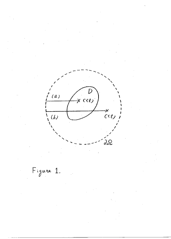
Figure 1: (a) $c(t)\in D$. (b) $c(t)\in\Omega\setminus\overline{D}$. Both cases satisfy $t(c;D)<t<1$.

This is an unexpected property of the indicator function and needs purely theoretical consideration. Their computation result does not cover this case since their approximation of the indicator function is too simple. The result is based on the discovery of the blowup of the sequence of the solutions of the Helmholtz equation given in Proposition 1.1 on the needle (Lemmas 2.1 and 2.2).

However, for the description of the result we do not make use of the formulation given above. We give a new and simpler formulation of the probe method. In the formulation, we do not make use of the impact parameter.

2 New formulation of the probe method

In this section, we introduce a new formulation of the probe method. Given a point $x\in\Omega$ let $N_{x}$ denote the set of all piecewise linear curves $\sigma:[0,\,1]\longmapsto\overline{\Omega}$ such that

(1) $\sigma(0)\in\partial\Omega$, $\sigma(1)=x$ and $\sigma(t)\in\Omega$ for all $t\in]0,\,1[$;

(2) $\sigma$ is injective.

We call $\sigma\in N_{x}$ a needle with tip at $x$. For the new formulation of the probe method we need the following.

Definition 2.1. Let $\sigma\in N_{x}$. We call the sequence $\xi=\{v_{n}\}$ of $H^{1}(\Omega)$ solutions of the Helmholtz equation a needle sequence for $(x,\sigma)$ if it satisfies, for each fixed compact set $K$ of ${\rm\bf R}^{m}$ with $K\subset\Omega\setminus\sigma([0,\,1])$

$$\lim_{n\longrightarrow\infty}(\|v_{n}(\,\cdot\,)-G_{k}(\,\cdot\,-x)\|_{L^{2}(K)}+\|\nabla\{v_{n}(\,\cdot\,)-G_{k}(\,\cdot\,-x)\}\|_{L^{2}(K)})=0.$$

Needless to say, the existence of the needle sequence is a consequence of Proposition 1.1. The problem is the behaviour of the needle sequence on the needle as $n\longrightarrow\infty$.

Here we make a definition. Let $b$ be a nonzero vector in ${\rm\bf R}^{m}$. Given $x\in{\rm\bf R}^{m}$, $\rho>0$ and $\theta\in]0,\pi[$ the set

$$V=\{y\in{\rm\bf R}^{m}\,|\,|y-x|<\rho\,\,\mbox{and}\,\,(y-x)\cdot\mbox{\boldmath$b$}>|y-x||\mbox{\boldmath$b$}|\cos(\theta/2)\}$$

is called a finite cone of height $\rho$, axis direction $b$ and aperture angle $\theta$ with vertex at $x$.

The two lemmas given below are the core of the new formulation of the probe method.

Lemma 2.1. Let $x\in\Omega$ be an arbitrary point and $\sigma$ be a needle with tip at $x$. Let $\xi=\{v_{n}\}$ be an arbitrary needle sequence for $(x,\sigma)$. Then, for any finite cone $V$ with vertex at $x$ we have

$$\lim_{n\longrightarrow\infty}\int_{V\cap\Omega}|\nabla v_{n}(y)|^{2}dy=\infty.$$

Proof. We employ a contradiction argument. Assume that the conclusion is not true. Then there exist $M>0$ and a sequence $n_{1}<n_{2}<\cdots\longrightarrow\infty$ such that

$$\int_{V\cap\Omega}|\nabla v_{n_{j}}(y)|^{2}dy<M,j=1,2,\cdots.$$

Take a sufficiently small open ball $B$ centred at $x$ with radius $R$ such that $\overline{B}\subset\Omega$ and $\sigma(]0,\,1])\cap B$ becomes a segment having $x$ as an end point. Then one can find a finite cone $V^{\prime}\subset V$ with vertex at $x$ such that, for every $\epsilon$ with $0<\epsilon<R$ $K_{\epsilon}\equiv\overline{V}^{\prime}\cap(\overline{B}\setminus B_{x}(\epsilon))\subset V\cap(\Omega\setminus\sigma(]0,\,1]))$ where $B_{x}(\epsilon)$ stands for the open ball centred at $x$ with radius $\epsilon$. Thus we have

$$\int_{K_{\epsilon}}|\nabla v_{n_{j}}(y)|^{2}dy<M,j=1,2,\cdots.$$

Since $\nabla v_{n_{j}}(\,\cdot\,)\longrightarrow\nabla G_{k}(\,\cdot\,-x)$ in $L^{2}(K_{\epsilon})$, we get

$$\int_{K_{\epsilon}}|\nabla G_{k}(y-x)|^{2}dy\leq M.$$

Since $\epsilon$ can be arbitrary small, applying Fatou’s lemma for $\epsilon=1/l$ as $l\longrightarrow\infty$ to the integral, we obtain

$$\int_{V^{\prime}\cap B}|\nabla G_{k}(y-x)|^{2}dy\leq M.$$

However, using polar coordinates centred at $x$ one can show that this left hand side is divergent. This is a contradiction and completes the proof.

$\Box$

Lemma 2.2. Let $x\in\Omega$ be an arbitrary point and $\sigma$ be a needle with tip at $x$. Let $\xi=\{v_{n}\}$ be an arbitrary needle sequence for $(x,\sigma)$. Then for any point $z\in\sigma(]0,\,1[)$ and open ball $B$ centred at $z$ we have

$$\lim_{n\longrightarrow\infty}\int_{B\cap\Omega}|\nabla v_{n}(y)|^{2}dy=\infty.$$

Proof.

Let $v$ be an arbitrary solution of the Helmholtz equation in $\Omega$. Note that $v$ can be identified with a smooth function in $\Omega$ and all the derivatives satisfy the Helmholtz equation in $\Omega$. Choose an open ball $B^{\prime}$ centred at $z$ such that $\overline{B}^{\prime}\subset B\cap\Omega$. Next choose a smaller open ball $B^{\prime\prime}$ centred at $z$ such that $\overline{B}^{\prime\prime}\subset B^{\prime}$. Applying (A.1) to the case when $W=B^{\prime}$ and $K=\overline{B}^{\prime\prime}$, we have

$$\int_{B^{\prime\prime}}|\nabla(\nabla v)|^{2}dy\leq C\int_{B^{\prime}}|\nabla v|^{2}dy.$$

Applying the trace theorem to $B^{\prime\prime}$, we have

$$\int_{\partial B^{\prime\prime}}|\nabla v|^{2}dS\leq C^{\prime}(\int_{B^{\prime\prime}}|\nabla v|^{2}dy+\int_{B^{\prime\prime}}|\nabla(\nabla v)|^{2}dy).$$

Choose a $C^{2}$ domain $U$ in such a way that $\Sigma\equiv\partial U\cap\partial B^{\prime\prime}$ has a positive surface measure on $\partial B^{\prime\prime}$, $\mbox{dist}\,(\partial U\setminus\Sigma,\sigma)>0$, $x\in U$ and $|U|$ is sufficiently small in the following sense:

$$\omega_{m}>k^{m}|U|$$

where $\omega_{m}$ is the volume of the unit ball in ${\rm\bf R}^{m}$. This last inequality implies that $0$ is not a Dirichlet eigenvalue of $\triangle+k^{2}$ in $U$ (see Lemma 1 in [14]).

Choose an open ball $B^{\prime\prime\prime}$ centered at $x$ such that $\overline{B}^{\prime\prime\prime}\subset U$ (see Figure 2 for the geometry).

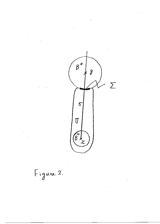
Figure 2: An illustration of $B^{\prime\prime},U,\Sigma$ and $B^{\prime\prime\prime}$.

Then (A.2) for the case when $W=U$ gives

$$\begin{array}[]{c}\displaystyle\int_{B^{\prime\prime\prime}}|\nabla v|^{2}dy\\ \\ \displaystyle\leq\int_{U}|\nabla v|^{2}dy\\ \\ \displaystyle\leq C^{\prime\prime}\int_{\partial U}|\nabla v|^{2}dS\\ \\ \displaystyle=C^{\prime\prime}(\int_{\Sigma}|\nabla v|^{2}dS+\int_{\partial U\setminus\Sigma}|\nabla v|^{2}dS)\\ \\ \displaystyle\leq C^{\prime\prime}(\int_{\partial B^{\prime\prime}}|\nabla v|^{2}dS+\int_{\partial U\setminus\Sigma}|\nabla v|^{2}dS).\end{array}$$

From (2.1), (2.2) and (2.3) we obtain the estimate of $\nabla v$ in $B^{\prime}$ in terms of $\nabla v$ in $B^{\prime\prime\prime}$ from below:

$$\int_{B^{\prime\prime\prime}}|\nabla v|^{2}dy\leq C^{\prime\prime\prime}(\int_{\partial U\setminus\Sigma}|\nabla v|^{2}dS+\int_{B^{\prime}}|\nabla v|^{2}dy).$$

Now set $v=v_{n}(\,\cdot\,)$. Since $\mbox{dis}\,(\partial U\setminus\Sigma,\sigma(]0,\,1]))>0$ and $\nabla v_{n}(\,\cdot\,)$ converges to $\nabla G_{k}(\,\cdot\,-x)$ in $H^{1}_{\mbox{loc}}(\Omega\setminus\sigma(]0,\,1]))$, the trace theorem gives

$$\lim_{n\longrightarrow\infty}\int_{\partial U\setminus\Sigma}|\nabla v_{n}(y)|^{2}dy=\int_{\partial U\setminus\Sigma}|\nabla G_{k}(y-x)|^{2}dy<\infty.$$

On the other hand, from Lemma 2.1, one knows that

$$\lim_{n\longrightarrow\infty}\int_{B^{\prime\prime\prime}}|\nabla v_{n}(y)|^{2}dy=\infty.$$

Thus from (2.4) for $v=v_{n}(\,\cdot\,)$, (2.5) and (2.6) we obtain the desired conclusion.

$\Box$

The argument given above can be applied to other elliptic equations and the elliptic systems by a suitable modification.

A combination of Lemmas 2.1 and 2.2 tells us that any needle sequence for any needle blows up on the needle. The needle sequence behaves like a beam! This is a new fact not mentioned in the previous papers about the probe method.

In order to describe our main result we introduce two positive constants appearing in two types of the Poincaré inequalities (e.g., see [15]). One is given in the following.

Proposition 2.1. For all $w\in H^{1}(\Omega\setminus\overline{D})$ with $w=0$ on $\partial\Omega$

$$\int_{\Omega\setminus\overline{D}}|w|^{2}dy\leq C_{0}(\Omega\setminus\overline{D})^{2}\int_{\Omega\setminus\overline{D}}|\nabla w|^{2}dy$$

where $C_{0}(\Omega\setminus\overline{D})$ is a positive constant independent of $w$.

Proof. This is nothing but a standard compactness argument.

$\Box$

The dependence of $C_{0}(\Omega\setminus\overline{D})$ on $\Omega\setminus\overline{D}$ should be clarified. However it is not the aim of this paper. Another is given in the following.

Proposition 2.2. Let $U$ be a bounded Lipschitz domain of ${\rm\bf R}^{m}$. For any $v\in H^{1}(U)$ we have

$$\int_{U}|v-v_{U}|^{2}dy\leq C(U)^{2}\int_{U}|\nabla v|^{2}dy$$

where $C(U)$ is a positive constant independent of $v$ and

$$v_{U}=\frac{1}{|U|}\int_{U}vdy.$$

Proof. Again, this is nothing but a standard compactness argument.

$\Box$

As a corollary we have

Proposition 2.3. Let $U$ be a bounded Lipschitz domain of ${\rm\bf R}^{m}$. For any $v\in H^{1}(U)$ and Lebesgue measurable $A\subset U$ with $|A|>0$ we have

$$\int_{U}|v-v_{A}|^{2}dy\leq C(U)^{2}(1+\frac{|U|^{1/2}}{|A|^{1/2}})^{2}\int_{U}|\nabla v|^{2}dy$$

where $C(U)$ is the same constant as that of Proposition 2.2 and

$$v_{A}=\frac{1}{|A|}\int_{A}vdy.$$

Proof. The following argument is taken from [13](see also [15] for an abstract version). Proposition 2.2 gives

$$\begin{array}[]{c}\displaystyle\|v-v_{A}\|_{L^{2}(U)}\leq\|v-v_{U}\|_{L^{2}(U)}+\|\frac{1}{|A|}\int_{A}(v-v_{U})dy\|_{L^{2}(U)}\\ \\ \displaystyle\leq C(U)\|\nabla v\|_{L^{2}(U)}+\frac{|U|^{1/2}}{|A|}|\int_{A}(v-v_{U})dy|\\ \\ \displaystyle\leq C(U)\|\nabla v\|_{L^{2}(U)}+\frac{|U|^{1/2}}{|A|^{1/2}}\|v-v_{U}\|_{L^{2}(U)}.\end{array}$$

Then again Proposition 2.2 gives the desired estimate.

$\Box$

We make use of the property that $\displaystyle C(U)^{2}(1+\frac{|U|^{1/2}}{|A|^{1/2}})^{2}$ continuously depends on $|A|$ for each fixed $U$.

Definition 2.2. Given $x\in\,\Omega$, needle $\sigma$ with tip $x$ and needle sequence $\xi=\{v_{n}\}$ for $(x,\sigma)$ define

$$I(x,\sigma,\xi)_{n}=\int_{\partial\Omega}\{(\Lambda_{0}-\Lambda_{D})\overline{f}_{n}\}f_{n}dS,\,n=1,2,\cdots$$

where

$$f_{n}(y)=v_{n}(y),\,\,y\in\,\partial\Omega.$$

$\{I(x,\sigma,\xi)_{n}\}_{n=1,2,\cdots}$ is a sequence depending on $\xi$ and $\sigma\in N_{x}$. We call the sequence the indicator sequence.

Now the main result is the following.

Theorem 2.1. Assume that $D$ is given by a union of finitely many bounded Lipschitz domains $D_{1},\cdots,D_{N}$ such that $\overline{D}_{j}\cap\overline{D}_{l}=\emptyset$ if $j\not=l$. Let $k\geq 0$ be small in the following sense:

$$k^{2}C_{0}(\Omega\setminus\overline{D})^{2}\leq 1$$

and

$$\min_{j}\{1-2k^{2}C(D_{j})^{2}(1+1)^{2}\}>0.$$

Then, given $x\in\Omega$ and needle $\sigma$ with tip at $x$ we have:

if $x\in\Omega\setminus\overline{D}$ and $\sigma(]0,1])\cap\overline{D}=\emptyset$, then for any needle sequence $\xi=\{v_{n}\}$ for $(x,\sigma)$ the sequence $\{I(x,\sigma,\xi)_{n}\}$ is convergent;

if $x\in\Omega\setminus\overline{D}$ and $\sigma(]0,1])\cap D\not=\emptyset$, then for any needle sequence $\xi=\{v_{n}\}$ for $(x,\sigma)$ we have $\lim_{n\longrightarrow\infty}I(x,\sigma,\xi)_{n}=\infty$;

if $x\in\overline{D}$, then for any needle sequence $\xi=\{v_{n}\}$ for $(x,\sigma)$ we have $\lim_{n\longrightarrow\infty}I(x,\sigma,\xi)_{n}=\infty$.

See Figure 3 for an illustration of three cases. This theorem does not cover the case when $x\in\Omega\setminus\overline{D}$ and $\sigma$ satisfies both $\sigma(]0,1])\cap D=\emptyset$ and $\sigma(]0,1])\cap\overline{D}\not=\emptyset$. However, this is quite an exceptional case. A similar theorem is valid in the case when $D$ is sound soft. In Theorem 1.1 from a technical reason we needed a restriction on the regularity of $\partial D$ ($C^{2}$ regularity). In Theorem 2.1 we need only Lipschitz regularity of $\partial D$ under smallness conditions (2.7) and (2.8) on $k$(however, being in attendance at the competition on relaxing the regularity of $\partial D$ is not the purpose of this paper). The piecewise linearity of the needle is introduced just for making the geometry simple and can be relaxed. However, from a practical point of view, it is enough.

Proof. From Proposition 2.3 we have

$$\begin{array}[]{c}\displaystyle\int_{D}|v|^{2}dy=\sum_{j}\int_{D_{j}}|v|^{2}dy\\ \\ \displaystyle\leq\sum_{j}2\int_{D_{j}}|v-v_{A_{j}}|^{2}dy+2\int_{D_{j}}|v_{A_{j}}|^{2}dy\\ \\ \displaystyle\leq\sum_{j}2C(D_{j})^{2}(1+\frac{|D_{j}|^{1/2}}{|A_{j}|^{1/2}})^{2}\int_{D_{j}}|\nabla v|^{2}dy+\sum_{j}2|D_{j}||v_{A_{j}}|^{2}\end{array}$$

where $A_{j}\subset D_{j}$ and satisfy $|A_{j}|>0$. Then from Proposition 2.1 and (A.3) we have the basic inequality

$$\begin{array}[]{c}\displaystyle\int_{\partial\Omega}\{(\Lambda_{0}-\Lambda_{D})\overline{f}\}fdS\displaystyle\geq(1-k^{2}C_{0}(\Omega\setminus\overline{D})^{2})\int_{\Omega\setminus\overline{D}}|\nabla w|^{2}dy\\ \\ \displaystyle+\sum_{j}(1-2k^{2}C(D_{j})^{2}(1+\frac{|D_{j}|^{1/2}}{|A_{j}|^{1/2}})^{2})\int_{D_{j}}|\nabla v|^{2}dy-2k^{2}|D|\sum_{j}|v_{A_{j}}|^{2}.\end{array}$$

Choose a sequence $\{K_{n}\}$ of compact sets of ${\rm\bf R}^{m}$ in such a way that $K_{n}\subset\Omega\setminus\sigma(]0,1])$; $\overline{K}_{n}\subset K_{n+1}$ for $n=1,\cdots$; $\Omega\setminus\sigma(]0,1])=\cup_{n=1}^{\infty}K_{n}$. Then $|K_{n}\cap D_{j}|\longrightarrow|D_{j}\setminus\sigma(]0,1])|=|D_{j}|$ as $n\longrightarrow\infty$ uniformly with $j=1,\cdots,N$. Thus one can take a large $n_{0}$ in such a way that the set $A_{j}\equiv K_{n_{0}}\cap D_{j}$ satisfies

$$\max_{j}\{2k^{2}(C(D_{j})^{2}(1+\frac{|D_{j}|^{1/2}}{|A_{j}|^{1/2}})^{2}-C(D_{j})^{2}(1+1)^{2})\}<\min_{j}\{1-2k^{2}C(D_{j})^{2}(1+1)^{2}\}.$$

We know that the sequences $\{(v_{n})_{A_{j}}\}$ for each $j=1,\cdots,N$ are always convergent since $\overline{A}_{j}\subset\Omega\setminus\sigma(]0,1])$. From (2.9) we have

$$I(x,\sigma,\xi)_{n}\geq NC\int_{D}|\nabla v_{n}|^{2}dy-2k^{2}|D|\sum_{j}|(v_{n})_{A_{j}}|^{2}$$

where

$$\begin{array}[]{c}\displaystyle C=\min_{j}\{1-2k^{2}C(D_{j})^{2}(1+1)^{2}\}\\ \\ \displaystyle-\max_{j}\{2k^{2}(C(D_{j})^{2}(1+\frac{|D_{j}|^{1/2}}{|A_{j}|^{1/2}})^{2}-C(D_{j})^{2}(1+1)^{2})\}>0.\end{array}$$

Then the blowup of $I(x,\sigma,\xi)_{n}$ comes from the blowup of the sequence

$$\int_{D}|\nabla v_{n}|^{2}dy.$$

If $x\in D$, then the blowup of the sequence given by (2.10) is a direct consequence of Lemma 2.1. If $x\in\partial D$, then the exists a finite cone $V$ at vertex at $x$ such that $V\subset D$. This is because of the Lipshitz regularity of $\partial D$. Then Lemma 2.1 gives the blowup of the sequence. Now consider the case when $x\in\Omega\setminus\overline{D}$. If $\sigma(]0,1])\cap\overline{D}=\emptyset$, then (A.3) and an argument given in [5] provide the convergence of $\{I(x,\sigma,\xi)_{n}\}$ for any needle sequence $\xi$. If $\sigma(]0,1])\cap D\not=\emptyset$, then there exists a point $z$ on $\sigma(]0,1[)\cap D$. Choose an open ball centred at $z$ in such a way that $B\subset D$. Then from Lemma 2.2 we see the blowup of the sequence given by (2.10).

$\Box$

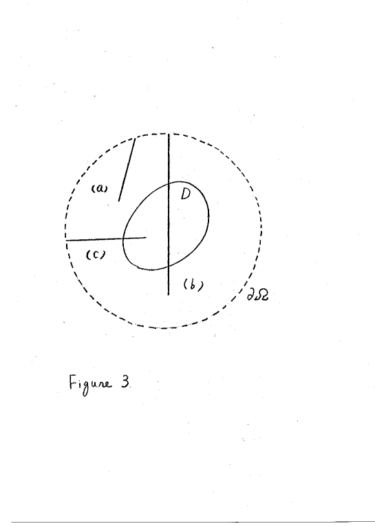
Figure 3: An illustration of three cases: (a) $x\in\Omega\setminus\overline{D}$ and $\sigma(]0,1])\cap\overline{D}=\emptyset$; (b) $x\in\Omega\setminus\overline{D}$ and $\sigma(]0,1])\cap D\not=\emptyset$; (c) $x\in\overline{D}$.

As a corollary of Theorem 2.1 we obtain the characterization of $\Omega\setminus\overline{D}$.

Corollary 2.1. Under the same assumptions as those of Theorem 2.1 we have: a point $x\in\Omega$ belongs to $\Omega\setminus\overline{D}$ if and only if there exist a needle $\sigma$ with tip at $x$ and needle sequence $\xi$ for $(x,\sigma)$ such that the sequence $\{I(x,\sigma,\xi)_{n}\}$ is bounded from above.

Proof. Since we have assumed that $\Omega\setminus\overline{D}$ is connected, if $x\in\Omega\setminus\overline{D}$, then, one can find a piecewise linear curve $\sigma:[0,\,1]\longrightarrow\overline{\Omega}\setminus D$ with $\sigma(0)\in\partial\Omega$, $\sigma(1)=x$ and $\sigma(t)\in\Omega\setminus\overline{D}$ for all $t\in\,]0,\,1[$. It is obvious that $\sigma$ can be chosen as an injective curve. This ensures the existence of a needle $\sigma$ with tip at $x$ such that $\sigma(]0,\,1])\subset\Omega\setminus\overline{D}$. Then from Theorem 2.1, one concludes the convergence of the indicator sequence for an arbitrary needle sequence $\xi$ for $(x,\sigma)$. Of course the existence of the needle sequence has been ensured. If $x\in\overline{D}$, then again from Theorem 2.1 we see that the indicator sequence for an arbitrary needle sequence for $(x,\sigma)$ for an arbitrary needle $\sigma$ with tip at $x$ blows up.

$\Box$

3 The reflected needle-an example

In this section we formulate a problem related to the behaviour of the sequence of reflected solutions by an obstacle introduced below (in the case $k=0$) and give an explicit answer in a simple situation. This is also an application of Lemmas 2.1 and 2.2.

Definition 3.1. We say that the sequence $\{g_{n}\}$ of $H^{1}(\Omega\setminus\overline{D})$ functions blows up at the point $z\in\overline{\Omega}\setminus D$ if for any open ball $B$ centered at $z$ it holds that

$$\lim_{n\longrightarrow\infty}\int_{B\cap(\overline{\Omega}\setminus D)}|\nabla g_{n}(y)|^{2}dy=\infty.$$

We call the set of all points $z\in\overline{\Omega}\setminus D$ such that $\{g_{n}\}$ blows up at $z$ the blowup set of $\{g_{n}\}$.

Given $x\in\Omega$, needle $\sigma$ with tip at $x$ and needle sequence $\xi=\{v_{n}\}$ for $(x,\sigma)$ let $u_{n}$ solve

$$\begin{array}[]{c}\displaystyle\triangle u=0\,\,\mbox{in}\,\Omega\setminus\overline{D},\\ \\ \displaystyle\frac{\partial u}{\partial\nu}=0\,\,\mbox{on}\,\partial D,\\ \\ \displaystyle u=v_{n}\,\,\mbox{on}\,\partial\Omega.\end{array}$$

The function $u_{n}-v_{n}$ is called the reflected solution by the obstacle $D$. It is easy to see that if $\sigma(]0,1])\cap\overline{D}=\emptyset$, then $\{u_{n}-v_{n}\}$ is bounded in $H^{1}(\Omega\setminus\overline{D})$ and thus the blowup set of sequence is empty.

We raise the following.

Problem. What can one say about the blowup set of $\{u_{n}-v_{n}\}$ when $\sigma(]0,1])\cap\overline{D}\not=\emptyset$?

Here we consider the problem in a simple case in two-dimensions. Let $R>\epsilon>0$. $\Omega$ and $D$ are given by the open discs centered at the origin with radius $R$ and $\epsilon$, respectively. We show that, in the case when $x\in D$, the blowup set of $\{u_{n}-v_{n}\}$ is given by a suitable curve in $\overline{\Omega}\setminus D$ obtained by transforming the part of needle $\sigma$ in $\overline{D}$. We call the curve the reflected needle.

Proposition 3.1. Let $\sigma$ be a needle with tip at $x\in D$ and satisfy the following: (1) $\sigma$ intersects with $\partial D$ only one time and (2) $\displaystyle\sigma(]0,1])\cap\{y\,|\,|y|\leq\frac{\epsilon^{2}}{R}\}=\emptyset$.

Then the blowup set of the sequence $\{u_{n}-v_{n}\}$ coincides with the curve $\sigma^{R}$ given by the formula (see Figure 4 for an illustration of $\sigma^{R}$)

$$\sigma^{R}=\{\frac{\epsilon^{2}y}{|y|^{2}}\,|\,y\in\sigma(]0,1])\cap\overline{D}\}.$$

Proof. Choose $\varphi\in C^{\infty}_{0}({\rm\bf R}^{2})$ in such a way that $\varphi=1$ in a neighbourhood of $\sigma(]0,1])\cap\overline{D}$ and $\varphi=0$ in a neighbourhood of the circle centered at the origin with radius $\displaystyle\epsilon^{2}/R$. Given needle sequence $\xi=\{v_{n}\}$ for $(x,\sigma)$ define

$$\tilde{v_{n}}(z)=\varphi(y)v_{n}(y),\,\,z\in\Omega\setminus\overline{D}$$

where

$$y=\frac{\epsilon^{2}z}{|z|^{2}}.$$

Note that this is nothing but the Kelvin transform of the function $\varphi v_{n}$ with respect to the circle centered at the origin with radius $\epsilon$.

Set

$$R_{n}(z)=u_{n}(z)-v_{n}(z)-\tilde{v_{n}}(z),\,\,z\in\Omega\setminus\overline{D}.$$

This function vanishes on $\partial\Omega$. A direct computation by using the polar coordinates around the origin gives the formula

$$\triangle_{z}\{g(y)\}=\frac{\epsilon^{4}}{|z|^{4}}(\triangle g)(y)$$

where $g$ is an arbitrary function in ${\rm\bf R}^{2}\setminus\{0\}$. Applying this formula to $g=\varphi v_{n}$, we have

$$(\triangle R_{n})(z)=-\frac{\epsilon^{4}}{|z|^{4}}\{(\triangle\varphi)(y)v_{n}(y)+2\nabla\varphi(y)\cdot\nabla v_{n}(y)\}.$$

This right-hand side is convergent as $n\longrightarrow\infty$ since both $\nabla\varphi(y)$ and $\triangle\varphi(y)$ vanish in a neighbourhood of the curve $\sigma(]0,1])\cap\overline{D}$; both $v_{n}(y)$ and $\nabla v_{n}(y)$ are convergent in $L^{2}(K)$ as $n\longrightarrow\infty$ where

$$K=\{y\,|\,\frac{\epsilon^{2}}{R}\leq|y|\leq\epsilon\,\,\mbox{and}\,\,\mbox{dis}\,(y,\sigma(]0,1])\cap\overline{D})\geq\eta\}\subset\Omega\setminus\sigma(]0,1])$$

and $0<\eta$.

A direct computation also gives

$$\frac{\partial R_{n}}{\partial\nu}(z)=-(1-\varphi(z))\frac{\partial v_{n}}{\partial\nu}(z)+\frac{\partial\varphi}{\partial\nu}(z)v_{n}(z),\,\,|z|=\epsilon.$$

This right hand sid is convergent in $H^{-1/2}(\partial D)$ since both $\partial\varphi/\partial\nu$ and $1-\varphi$ vanish for $z$ close to the single point in the set $\sigma(]0,1])\cap\partial D$. Then the well posedness of the mixed boundary value problem yields that the sequence $\{R_{n}\}$ is bounded in $H^{1}(\Omega\setminus\overline{D})$. Then from Lemmas 2.1 and 2.2 one obtains the desired conclusion.

$\Box$

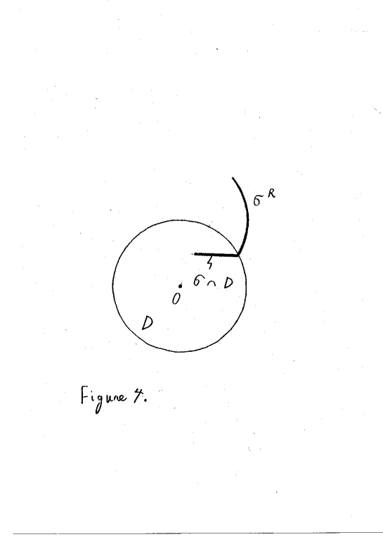
Figure 4: An illustration of $\sigma^{R}$.

We think that Proposition 3.1 is a special case of a more general theorem that shall give the description of the blowup set of $\{u_{n}-v_{n}\}$ by using a curve obtained by a rule. In a forthcoming paper we will consider the problem of seeking such a rule for general $D$, $\Omega$ and $k>0$.

4 Remark

It is possible to obtain the corresponding results in other applications of the probe method (see [3, 7]). For example, consider the Dirichlet-to-Neumann map $\Lambda_{\gamma}$ for the equation $\nabla\cdot\gamma\nabla u=0$ in $\Omega$. Here $\gamma=\gamma(y)$ denotes the electrical conductivity. Assume that $\gamma$ takes the form: $\gamma(y)=1,\,y\in\,\Omega\setminus D$ and $1+h(y),\,\,y\in\,D$ where $h(y)$ is given by a function in $L^{\infty}(D)$ satisfying $\mbox{ess}\,\inf_{y\in D}(1+h(y))>0$ and the global jump condition: $h(y)\geq C$ a.e. in $D$ or $-h(y)\geq C$ a.e. in $D$ for a positive constant $C$. We obtain Theorem 4.1. A point $x\in\Omega$ belongs to $\Omega\setminus\overline{D}$ if and only if there exist a needle $\sigma$ with tip at $x$ and needle sequence $\xi=\{v_{n}\}$ for $k=0$ such that the sequence $\{I(x,\sigma,\xi)_{n}\}$ given by the formula

$$\begin{array}[]{c}\displaystyle I(x,\sigma,\xi)_{n}=\int_{\partial\Omega}\{(\Lambda_{\gamma}-\Lambda_{1})f_{n}\}f_{n}dS,\\ \\ \displaystyle f_{n}(y)=v_{n}(y),\,\,y\in\partial\Omega,\end{array}$$

is bounded. Moreover given $x\in\Omega$ and needle $\sigma$ with tip at $x$ we have that

if $x\in\Omega\setminus\overline{D}$ and $\sigma(]0,1])\cap\overline{D}=\emptyset$, then for any needle sequence $\xi=\{v_{n}\}$ for $(x,\sigma)$ the sequence $\{I(x,\sigma,\xi)_{n}\}$ is convergent

if $x\in\Omega\setminus\overline{D}$ and $\sigma(]0,1])\cap D\not=\emptyset$, then for any needle sequence $\xi=\{v_{n}\}$ for $(x,\sigma)$ we have $\lim_{n\longrightarrow\infty}|I(x,\sigma,\xi)_{n}|=\infty$

if $x\in\overline{D}$, then for any needle sequence $\xi=\{v_{n}\}$ for $(x,\sigma)$ we have $\lim_{n\longrightarrow\infty}|I(x,\sigma,\xi)_{n}|=\infty$.

This theorem suggests that the new formulation of the probe method can probably be considered as a final generalization of the enclosure method introduced in [6]. The needle sequences play the role similar to the special harmonic functions coming from Mittag-Leffler’s function in a generalized enclosure method given in [8, 9]. The proof is a direct consequence of the system of the integral inequalities ([2]) and Lemmas 2.1 and 2.2 for $k=0$.

We point out that the behaviour of $\{I(x,\sigma,\xi)_{n}\}$ for general $x\in\overline{D}$ is not clear without a global assumption on $h$ in $D$. However, one can easily deduce that if $h$ or $-h$ has a positive lower bound in a neighbourhood of $\sigma(]0,\,1])\cap\overline{D}$, then $\lim_{n\longrightarrow\infty}|I(x,\sigma,\xi)_{n}|=\infty$.

In my opinion, it is impossible to know the behaviour of $I(x,\sigma,\xi)_{n}$ as $n\longrightarrow\infty$ for $x\in\overline{D}$ from the property of the needle sequence in the case when both $h$ and $-h$ do not have a positive lower bound in any neighbourhood of $\sigma(]0,\,1])\cap\overline{D}$. For this purpose we have to study the behaviour of the sequence of reflected/refracted solutions by the obstacles, inclusions and cracks. We also think that the study may enable us to drop the restriction on $k$ given by (2.7) and (2.8).

   

Acknowledgement

This research was partially supported by Grant-in-Aid for Scientific Research (C)(2) (No. 15540154) of Japan Society for the Promotion of Science. The author thanks Klaus Erhard and Roland Potthast for providing me with a preprint of [1] and the anonymous referees for their valuable comments and suggestions for improvement of the original manuscript.

   

5 Appendix

A.1. Remark. In the proof of Theorem 4 of [5] some important explanations described below are missing.

(1) $f$ in (A.1) of the paper should belong to $\{H^{1}(U)\}^{*}$ and satisfy $f(v|_{U})=0$ for all $v|_{U}\in\,Y$;

(2) the right hand side of (A.1) of the paper defines a bounded linear functional on $H^{1}_{0}(\Omega)$.

A.2. Estimates.

Proposition A.1. Let $W$ be a bounded domain with $C^{2}$ boundary of ${\rm\bf R}^{m}$. Let $v\in H^{1}(W)$ satisfy $\triangle v+k^{2}v=0$ in $W$. Then, for any compact set $K$ of ${\rm\bf R}^{m}$ with $K\subset W$ there exists a positive constant $C^{\prime}=C^{\prime}(K,W)$ independent of $v$ such that

$$\int_{K}|\nabla v|^{2}dy\leq C^{\prime}\int_{W}|v|^{2}dy.$$

Moreover, assume that $0$ is not a Dirichlet eigenvalue of $\triangle+k^{2}$ in $W$. Then there exists a positive constant $C=C(W)$ independent of $v$ such that

$$\int_{W}|v|^{2}dy\leq C\int_{\partial W}|v|^{2}dS.$$

Proof. First we prove (A.1). Let $\varphi\in C^{\infty}_{0}(W,{\rm\bf R})$. Multiply the equation $\triangle v+k^{2}v=0$ in $W$ by $\varphi^{2}\overline{v}$ and integrate the resultant equation over $W$. Integration by parts gives

$$\int_{W}|\nabla v|^{2}\varphi^{2}dy\leq C\int_{W}|v|^{2}|\nabla\varphi|^{2}dy+\int_{W}k^{2}|v|^{2}\varphi^{2}dy.$$

Choose $\varphi\in C^{\infty}_{0}(W)$ in such a way that $\varphi=1$ on $K$ and $0\leq\varphi\leq 1$. Then one gets (A.1).

Let $z\in H^{2}(W)$ solve

$$\begin{array}[]{c}\displaystyle\triangle z+k^{2}z=\overline{v},\,\,\mbox{in}\,W,\\ \\ \displaystyle z=0\,\,\mbox{on}\,\partial W.\end{array}$$

Then we have

$$\begin{array}[]{c}\displaystyle\int_{W}|v|^{2}dy=\int_{W}(\triangle z+k^{2}z)vdy\\ \\ \displaystyle=\int_{\partial W}\frac{\partial z}{\partial\nu}vdS-\int_{W}\nabla z\cdot\nabla vdy+\int_{W}k^{2}zv\\ \\ \displaystyle=\int_{\partial W}\frac{\partial z}{\partial\nu}vdS\end{array}$$

and the trace theorem yields

$$\begin{array}[]{c}\displaystyle\|v\|^{2}_{L^{2}(W)}\leq\int_{\partial W}|\frac{\partial z}{\partial\nu}||v|dS\\ \\ \displaystyle\leq\|\nabla z\|_{L^{2}(\partial W)}\|v|_{\partial W}\|_{L^{2}(\partial W)}\\ \\ \displaystyle\leq C_{1}\|z\|_{H^{2}(W)}\|v|_{\partial W}\|_{L^{2}(\partial W)}\\ \\ \displaystyle\leq C_{2}\|v\|_{L^{2}(W)}\|v|_{\partial W}\|_{L^{2}(\partial W)}.\end{array}$$

Thus we obtain (A.2).

$\Box$

The reader can see this type of argument for the proof of this proposition, e.g., in [10].

A.3. An integral identity.

The identity below has been established in [5].

Proposition A.2. For all $f\in H^{1/2}(\partial\Omega)$

$$\begin{array}[]{c}\displaystyle\int_{\partial\Omega}\{(\Lambda_{0}-\Lambda_{D})\overline{f}\}fdS\\ \\ \displaystyle=\int_{\Omega\setminus\overline{D}}|\nabla(u-v)|^{2}dy-k^{2}\int_{\Omega\setminus\overline{D}}|u-v|^{2}dy\\ \\ \displaystyle+\int_{D}|\nabla v|^{2}dy-k^{2}\int_{D}|v|^{2}dy\end{array}$$

where $u$ solves

$$\begin{array}[]{c}\displaystyle(\triangle+k^{2})u=0\,\,\mbox{in}\,\,\Omega\setminus\overline{D},\\ \\ \displaystyle u=f\,\,\mbox{on}\,\,\partial\Omega,\\ \\ \displaystyle\frac{\partial u}{\partial\nu}=0\,\,\mbox{on}\,\,\partial D;\end{array}$$

$v$ solves

$$\begin{array}[]{c}\displaystyle(\triangle+k^{2})v=0\,\,\mbox{in}\,\,\Omega,\\ \\ \displaystyle v=f\,\,\mbox{on}\,\,\partial\Omega.\end{array}$$

e-mail address

ikehata@math.sci.gunma-u.ac.jp