Noise stability of synchronization and optimal network structures

Abstract

We provide a theoretical framework for quantifying the expected level of synchronization in a network of noisy oscillators. Through linearization around the synchronized state, we derive the following quantities as functions of the eigenvalues and eigenfunctions of the network Laplacian using a standard technique for dealing with multivariate Ornstein-Uhlenbeck processes: the magnitude of the fluctuations around a synchronized state and the disturbance coefficients $\alpha_{i}$ that represent how strongly node $i$ disturbs the synchronization. With this approach, we can quantify the effect of individual nodes and links on synchronization. Our theory can thus be utilized to find the optimal network structure for accomplishing the best synchronization. Furthermore, when the noise levels of the oscillators are heterogeneous, we can also find optimal oscillator configurations, i.e., where to place oscillators in a given network depending on their noise levels. We apply our theory to several example networks to elucidate optimal network structures and oscillator configurations.

Synchronization of rhythmic elements is essential in many systems. To function properly and well, rhythmic elements are required to maintain an appropriate synchronization pattern precisely. What is the best network structure for accomplishing the best synchronization? In other word, which elements should each element have look at? Here, we develop a measure to quantify the precision of synchronization for a given network. Using this measure, we can quantitatively compare the stability of different networks and find the optimal network structure. We can also determine where reliable or unreliable elements should be placed in a given network.

I Introduction

Synchronization of rhythmic elements, or oscillators, is ubiquitous and underlies various important functions Winfree (2001); Kuramoto (1984); Pikovsky, Rosenblum, and Kurths (2001). For example, biological rhythms, including circadian rhythms and heartbeats, are generated by a population of cells acting periodically and synchronously Winfree (2001); Glass (2001). Synchronization also plays a vital role in locomotion Hoyt and Taylor (1981); Taga, Yamaguchi, and Shimizu (1991); Ijspeert (2008). For each gait, the limbs perform rhythmic movements and maintain a certain synchronization pattern. Synchronization is also essential in various artistic performances, including those by orchestras, choruses, and dancers Stoklasa, Liebermann, and Fischinger (2012); Miyashita et al. (2011); Wuyts and Buekers (1995).

In any example, to function properly and well, a population of oscillators is required to maintain an appropriate synchronization pattern, such as perfect synchrony, wave-like patterns, or more complex patterns. However, oscillators are inevitably exposed to noise. For example, the activity of a cell involves fluctuations due to various types of intrinsic and extrinsic noises Elowitz et al. (2002); Faisal, Selen, and Wolpert (2008). Limbs experience perturbations from the ground or the surrounding fluid. Humans are unable to generate perfectly rhythmic actions, even in the absence of external disturbances. Such randomness disturbs synchronization and may hamper performance. Synchronization patterns must therefore be highly stable against the noise affecting individual oscillators. Since synchronization occurs because of the interactions between the oscillators, the structure of the interaction network is expected to strongly influence the synchronization stability.

The local stability problem of synchronous states is generally reduced to an eigenvalue problem of a particular class of stability matrices, which is often referred to as a network Laplacian $L$ or a Kirchhoff matrix Arenas et al. (2008). This class of matrices appears in a variety of dynamical processes on networks and lattices, such as random walks Masuda, Porter, and Lambiotte (2017), consensus problems Olfati-Saber, Fax, and Murray (2007), and reaction-diffusion on networks Nakao and Mikhailov (2010). Consequently, there is a long history of studies of network Laplacians. In particular, the properties of the eigenvalues, or the spectrum of the network Laplacians, have been studied intensively Mohar et al. (1991); Chung (1997). The smallest non-zero eigenvalue of $L$, termed $\lambda_{2}$ in this paper, often attracts attention because its inverse provides a typical timescale that facilitates relaxation to a synchronized state Arenas et al. (2008). It also provides a condition for the change of stability caused by variations in the system parameters, including changes in the network structure Arenas et al. (2008). For the synchronization of chaotic oscillators, the ratio of the smallest to the largest eigenvalues, $\lambda_{2}/\lambda_{N}$, also plays an important role in determining the stability of the network Barahona and Pecora (2002), and the optimal network structure that minimizes this ratio has been investigated Nishikawa and Motter (2006).

However, when we are concerned with the extent to which the synchronization pattern is precisely maintained in a network of noisy oscillators, knowledge of just a few dynamical modes is not sufficient, because every dynamical mode is excited at every time by noise. Therefore, we provide a theoretical framework here for quantifying the magnitude of the fluctuations around a synchronous state. Our framework is based on phase models, which describe oscillator networks to a good approximation when the coupling and noise are sufficiently weak. We are particularly interested in the case in which oscillators have different noise strengths, because individual cells and humans experience different noise levels. We derive an expression for the magnitude of the fluctuations in an entire network as the weighted sum of the noise intensities of individual oscillators. This weight, termed the “disturbance coefficient” of a node, describes the extent to which an oscillator placed at that node disturbs the synchronization of the network. The disturbance coefficients of a network depend on the network structure, which may differ significantly among the nodes. Our theory can thus be utilized to find an optimal network structure that minimizes the fluctuation level and to find an optimal oscillator configuration; i.e., to determine at which nodes oscillators with higher or lower noise strengths should be placed in a given network.

II Theory

We first present our theoretical framework; we outline our theory before going into detail about it. In Sec. II.1, We begin by considering a particular class of phase models that describe the networks of $N$ interacting oscillators admitting perfect synchrony (i.e., an in-phase state) in the absence of noise. The level of synchronization can be characterized by the Kuramoto order parameter $r(t)$ $(0\leq r\leq 1)$, which assumes $r=1$ in the absence of noise and typically decreases as the strength of the noise increases. We are concerned with the expectation (i.e., the ensemble average) of $r$ for a given network and noise strength. In Sec. II.2, we derive an expression for this quantity, denoted by $Q$, by assuming weak noise and linearizing the system around the in-phase state. The problem with which we are concerned is then reduced to a general class of linear dynamical systems, which are described by a network Laplacian $L$. We derive $Q$ as a function of the eigenvalues and eigenvectors of $L$ and of the individual noise strengths $\eta_{i}$ ($1\leq i\leq N$). In the derivation, we assume $L$ is diagonalizable; however, we also propose a method to treat a non-diagonalizable Laplacian $L$ (Sec. II.3). In Sec. II.4, we show that our theory can also be applied to a more general class of phase models and synchronized states.

Examples and numerical verification follow in Secs. III and  IV, respectively.

II.1 Synchronization of oscillator networks

We consider a network of self-sustained oscillators that are subjected to independent noise. When the coupling and noise are weak, the system is described by a phase model to a good approximation Winfree (1967); Kuramoto (1984). By further assuming that all the oscillators are identical, it is appropriate to consider the system

$$\dot{\phi_{i}}(t)=\omega+\sum_{j=1}^{N}A_{ij}f(\phi_{j}-\phi_{i})+\xi_{i}(t),$$ (1)

where $\phi_{i}$ $(1\leq i\leq N)$ is the phase of the $i$th oscillator, $\omega$ is the natural frequency, $A_{ij}\geq 0$ is the weight of a directed edge that describes the strength of the coupling from the $j$th oscillator to the $i$th oscillator, $f$ is a $2\pi$-periodic function, and the $\xi_{i}$ represents independent Gaussian white noise. The latter variables satisfy

$$\langle\xi_{i}(t)\rangle=0,\quad\langle\xi_{i}(t)\xi_{j}(s)\rangle=\eta_{i}\delta_{ij}\delta(t-s),$$ (2)

where $\langle\cdot\rangle$ represents the expectation value and $\eta_{i}\geq 0$ is the strength of the noise to which the $i$th oscillator is subjected. We assume $f(0)=0$ and $f^{\prime}(0)>0$. The former implies that the coupling vanishes when all the oscillators are in phase; i.e., $\phi_{i}=\phi_{j}$ for all $i$ and $j$. The latter implies that the in-phase state of two mutually coupled oscillators is linearly stable in the absence of noise. This type of coupling typically arises in chemical and biological oscillators coupled electrically or diffusively Kopell and Ermentrout (2004); Kiss, Zhai, and Hudson (2005); Miyazaki and Kinoshita (2006); Kori et al. (2014); Stankovski et al. (2017). We set $f^{\prime}(0)=1$ without loss of generality. Our theory may be generalized to more general phase models, as described in Sec. II.4.

In this setting, our oscillator network has an in-phase state (i.e., the completely synchronized state), which is given by

$$\phi_{i}=\omega t+C,$$ (3)

where $C$ is an arbitrary constant. We assume that this state is stable, which holds true under mild conditions, as detailed in Sec. II.2. We also assume that the noise is sufficiently weak so that the system fluctuates weakly around the in-phase state. We are concerned with the magnitude of the fluctuations of this system.

To quantify the level of synchronization, we introduce the Kuramoto order parameter $r$ $(0\leq r\leq 1)$, defined as

$$re^{i\theta}=\frac{1}{N}\sum_{j=1}^{N}e^{i\phi_{j}},$$ (4)

where $\theta$ can be interpreted as the mean phase of the oscillators. When the system is nearly in-phase, $\phi_{j}-\theta$ is small. By rewriting Eq. (4) as $r=\frac{1}{N}\sum_{j=1}^{N}e^{i(\phi_{j}-\theta)}$ and dropping the terms of $O\left[(\phi_{j}-\theta)^{3}\right]$, we obtain

$$r =\frac{1}{N}\sum_{j=1}^{N}\left(1-\frac{(\phi_{j}-\theta)^{2}}{2}+i(\phi_{j}-\theta)\right).$$ (5)

By equating the imaginary parts of both sides, we find

$$\theta=\frac{1}{N}\sum_{j=1}^{N}\phi_{j}.$$ (6)

By equating the real parts of both sides and introducing $x_{i}=\phi_{i}-\omega t$, we obtain

$$r=\frac{1}{N}\sum_{j=1}^{N}\left[1-\frac{(x_{j}-\overline{x})^{2}}{2}\right],$$ (7)

where

$$\overline{x}=\frac{1}{N}\sum_{j=1}^{N}x_{j}.$$ (8)

The expectation value of $r$ is thus given by

$$\langle r\rangle=1-\frac{Q}{2},$$ (9)

where

$$Q=\frac{1}{N}\sum_{j=1}^{N}\langle(x_{j}-\overline{x})^{2}\rangle.$$ (10)

The quantity $Q$ can be interpreted as the variance of the phases $\phi_{i}$ when the system is nearly in phase. The smaller the value of $Q$, the better the system is synchronized. Below, based on linearization and diagonalization of our model, we derive an expression for $Q$.

II.2 Linearized system

We linearize Eq. (1) for small phase differences $\phi_{j}-\phi_{i}$ ($1\leq i,j\leq N$) and substitute $\phi_{i}=\omega t+x_{i}$ to obtain

$$\dot{x_{i}}=\sum_{j=1}^{N}A_{ij}(x_{j}-x_{i})+\xi_{i},$$ (11)

or

$$\dot{\bm{x}}=-L\bm{x}+\bm{\xi},$$ (12)

where $\bm{x}=(x_{1},\ldots,x_{N})^{\rm T}$ and $\bm{\xi}=(\xi_{1},\ldots,\xi_{N})^{\rm T}$, and the network Laplacian $L=(L_{ij})$ is given by

$$L_{ij}=\begin{cases}-A_{ij}&\mathrm{for}\,i\neq j,\\ \displaystyle\sum_{i^{\prime}\neq i}A_{ii^{\prime}}&\mathrm{for}\,i=j.\end{cases}$$ (13)

Equation (12) is a particular class of multivariate Ornstein-Uhlenbeck processes. When $L$ is diagonalizable, which we assume below, many quantities can be derived analytically Risken (1996). We denote the eigenvalues of $L$ by $\lambda_{n}$ $(1\leq n\leq N)$ and their corresponding right and left eigenvectors by $\bm{u}^{(n)}=\left(u_{1}^{(n)},u_{2}^{(n)},\ldots,u_{N}^{(n)}\right)^{\rm T}$ and $\bm{v}^{(n)}=\left(v_{1}^{(n)}\;v_{2}^{(n)}\;\cdots\;v_{N}^{(n)}\right)$, respectively; i.e.,

$$L\bm{u}^{(n)} =\lambda_{n}\bm{u}^{(n)},$$ (14)

$$\bm{v}^{(n)}L =\lambda_{n}\bm{v}^{(n)}.$$ (15)

Note that $\bm{u}^{(n)}$ and $\bm{v}^{(n)}$ are column and row vectors, respectively. Because $L$ is assumed to be diagonalizable, these eigenvectors can be chosen to be bi-orthonormal; i.e.,

$$\bm{v}^{(m)}\bm{u}^{(n)}=\delta_{mn}.$$ (16)

For a symmetric matrix $L$, the right and left eigenvectors are parallel to each other; thus, we set $\bm{v}^{(m)}=\bm{u}^{(m){\rm T}}$ and normalize the eigenvectors as $\bm{u}^{(m)}\cdot\bm{u}^{(n)}=\delta_{mn}$.

One of the eigenvalues of $L$ is zero; it is denoted by $\lambda_{1}=0$, and its corresponding right eigenvector is denoted by

$$\bm{u}^{(1)}=(1,1,\cdots,1)^{\rm T}.$$ (17)

When the in-phase state is stable, we have

$$0=\lambda_{1}<\mathrm{Re}\,\lambda_{2}\leq\mathrm{Re}\,\lambda_{3}\leq\ldots\leq\mathrm{Re}\,\lambda_{N},$$ (18)

where $\mathrm{Re}\,\lambda$ denotes the real part of $\lambda$. When $A_{ij}\geq 0$ for $1\leq i,j\leq N$, Eq. (18) holds true under the following mild condition: all the nodes are reachable from a single node along directed paths, where the directed path from node $j$ to $i$ is assumed to be present when $A_{ij}>0$ Ermentrout (1992); Arenas et al. (2008). Strongly connected networks suffice this condition.

By diagonalizing Eq. (12) using the eigenvectors defined above, we can solve Eq. (12) to derive the expression for $Q$ given in Eq. (10). As shown in detail in Appendix A, we obtain

$$Q =\sum_{i=1}^{N}\alpha_{i}\eta_{i},$$ (19a)

$$\alpha_{i} =\sum_{m,n=2}^{N}\frac{\overline{u^{(m)}u^{(n)}}-\overline{u^{(m)}}\ \overline{u^{(n)}}}{\lambda_{m}+\lambda_{n}}v_{i}^{(m)}v_{i}^{(n)}.$$ (19b)

where $\overline{u^{(m)}}=\frac{1}{N}\sum_{i=1}^{N}u_{i}^{(m)}$, and $\overline{u^{(m)}u^{(n)}}=\frac{1}{N}\sum_{i=1}^{N}u_{i}^{(m)}u_{i}^{(n)}$. Thus, as given in Eq. (19), fluctuations around the synchronous state are expressed as the summation of individual noise strengths $\eta_{i}$, each weighted by $\alpha_{i}$, which we call the disturbance coefficient of a node $i$. Oscillators placed at the nodes with larger values of $\alpha_{i}$ tend to disturb the synchronization more strongly.

For a symmetric matrix $L$, Eq. (19b) reduces to (see Appendix A)

$$\alpha_{i}=\frac{1}{2N}\sum_{n=2}^{N}\frac{\left(u_{i}^{(n)}\right)^{2}}{\lambda_{n}}.$$ (20)

Further, by assuming homogeneous noise strengths, i.e., $\eta_{i}=\eta$, Eq. (19a) reduces to

$$Q=\frac{\eta}{2N}\sum_{n=2}^{N}\frac{1}{\lambda_{n}}.$$ (21)

Equation (21) has already been derived in Ref. Yanagita and Ichinomiya (2014), which focuses on symmetric Laplacians $L$ and homogeneous noise strengths.

II.3 The non-diagonalizable case

Our derivation above was based on the assumption that $L$ is diagonalizable. However, we may also be interested in networks that yield non-diagonalizable matrices $L$, which we consider in Sec. III.3. Even when $L$ is non-diagonalizable, we may obtain values for $Q$ and $\alpha_{i}$ in the following manner.

We assume that we have a non-diagonalizable Laplacian $L$. Then, we introduce $M$ extra parameters $\bm{p}=(p_{1},p_{2},\ldots,p_{M})\in\mathbb{R}^{M}$ and add $p_{k}$ to $L_{i_{k}j_{k}}$ ($1\leq k\leq M,1\leq i_{k}\leq N,1\leq j_{k}\leq N$). We denote the resulting matrix by $L(\bm{p})$. By construction, we have $L=L(\bm{0})$. We may obtain a diagonalizable matrix $L(\bm{p})$ if $M$ is sufficiently large and an appropriate set $\{(i_{k},j_{k})\}$ is chosen. We denote the resulting expression for $Q$ for $L(\bm{p})$ by $Q(\bm{p})$. We may expect $Q(\bm{0})$ to describe the $Q$ value for the non-diagonalizable $L(\bm{0})$.

We show that this method indeed works for the network considered in Sec. III.3, which we verify numerically in Sec. IV.

II.4 Generalization

In Sec. II.1, we considered a particular class of phase models, represented by Eq. (12), in order to consider a stable in-phase state. Our theory can also be extended to a more general class of phase models in which a stable phase-locked state exists. Important examples include phase waves and spirals in spatially extended systems Ermentrout (1992); Masuda, Kawamura, and Kori (2010).

We consider

$$\dot{\phi_{i}}(t)=\omega_{i}+\sum_{j=1}^{N}B_{ij}f_{ij}(\phi_{j}-\phi_{i})+\xi_{i}(t),$$ (22)

where $\omega_{i}$ is the natural frequency of oscillator $i$, $B=(B_{ij})$ is the adjacency matrix, and $f_{ij}$ is a $2\pi$-periodic function that describes the coupling from oscillator $j$ to oscillator $i$. We assume that in the absence of noise, Eq. (1) has a phase-locked state

$$\phi_{i}(t)=\Omega t+\psi_{i}^{*}$$ (23)

for $1\leq i\leq N$. Here, $\Omega$ is the frequency of the synchronized state and the $\psi_{i}^{*}$ are constant phase offsets, which are found as solutions to the following set of equations: $\omega_{i}+\sum_{j=1}^{N}B_{ij}f_{ij}(\psi_{j}^{*}-\psi_{i}^{*})=\Omega$ ($1\leq i\leq N$). Then, introducing $x_{i}(t)=\phi_{i}(t)-\Omega t-\psi_{i}^{*}$ and linearizing Eq. (1) for small $x_{j}-x_{i}$, we obtain exactly the same linear model as given by Eq. (12), where now

$$A_{ij}=B_{ij}f_{ij}^{\prime}(\psi_{j}^{*}-\psi_{i}^{*}).$$ (24)

For such a phase-locked state, the magnitude of the fluctuations around the synchronized state can be quantified by Eq. (10). Therefore, the theory presented in Sec. II.2 does not require any modification. Only the interpretation of $A_{ij}$ is slightly changed, as indicated in Eq. (24).

III Examples

Utilizing our theory, we now look for optimal network structures for several types of networks under various constraints. We assume that each oscillator has its own inherent noise strength and that we are allowed to place an oscillator at an arbitrary node in the network to make $Q$ as small as possible; i.e., we also consider the optimal configuration of oscillators.

III.1 Two nodes with two weighted edges

Figure 1: Network of two nodes and two edges, in which $Q$ is inversely proportional to $a+b$ and does not depend on the ratio of $a$ to $b$.

We first consider a very simple network; i.e., two nodes with two weighted edges (Fig. 1). The corresponding Laplacian is

$$L=\left(\scalebox{1.0}{$\displaystyle\begin{array}[]{cc}b&-b\\ -a&a\end{array}$}\right),$$ (27)

which has the eigenvalues $\lambda_{1}=0$ and $\lambda_{2}=a+b$. Thus, the stability condition holds true when $a+b>0$. The corresponding right and left eigenvectors are

$$\bm{u}^{(1)}=\left(1,1\right)^{\rm T},\bm{u}^{(2)}=\left(-\frac{b}{a},1\right)^{\rm T},$$ (28)

$$\bm{v}^{(1)}=\left(\frac{a}{b}\quad 1\right),\bm{v}^{(2)}=\left(-1\quad 1\right).$$ (29)

Substituting these expressions into Eq. (19), we obtain

$$Q=\frac{\eta_{1}+\eta_{2}}{16(a+b)}.$$ (30)

Here, $Q$ decreases with increasing $a+b$, in accordance with the behavior of the eigenvalues and is independent of the ratio of $a$ to $b$; i.e., there is no network-structure dependence in this particular example. Moreover, the disturbance coefficients $\alpha_{1}$ and $\alpha_{2}$ are identical, so $Q$ is independent of the oscillator configuration.

III.2 Three nodes with three weighted edges

Figure 2: Networks of three nodes and three edges. (A) Feedback network. (B) Feedfoward network. The optimal weight distribution under the constraint $a+b+c=1$ and $\eta_{i}=\eta$ ($i=1,2,3$) is (A) $a=b=c=\frac{1}{3}$ and (B) $a=c=\frac{1}{2}$, $b=0$. The corresponding $Q$ value is $\frac{\eta}{3}$ for both networks; these two optimal networks are equivalently noise-tolerant.

We next consider two networks consisting of three nodes and three edges, as shown in Fig. 2. The network motifs shown in Fig. 2(A) and (B) appear abundantly in biological networks, and they are termed “feedback” and “feedforward” networks, respectively Milo et al. (2002). By calculating the eigenvalues and eigenvectors of the corresponding network Laplacians, we obtain the following expressions for $Q$ for Figs. 2(A) and (B):

$$Q^{\mathrm{(A)}} =\frac{(a+b)\eta_{1}+(b+c)\eta_{2}+(c+a)\eta_{3}}{18(ab+bc+ca)},$$ (31)

$$Q^{\mathrm{(B)}} =\frac{1}{18\left(a^{2}b+ab^{2}+a^{2}c+ac^{2}+2abc\right)}$$

$$\qquad\left(\left(a^{2}+b^{2}+c^{2}+2ab+bc\right)\eta_{1}\right.$$

$$\qquad\ +\left(b^{2}+c^{2}+ab+bc+ca\right)\eta_{2}$$

$$\qquad\ \left.+\left(a^{2}+ab+ac\right)\eta_{3}\right),$$ (32)

respectively. Because the disturbance coefficients $\alpha_{i}$ (i.e., the coefficients of $\eta_{i}$) are different for $i=1,2,3$, the $Q$ values for these cases depend on the oscillator configuration. By restricting ourselves to the case of identical noise strengths, i.e., $\eta_{i}=\eta$ ($i=1,2,3$), we look for the optimal structures under the constraint $a+b+c=1$. By using, the method of Lagrange multipliers, for example, we find that (A) $a=b=c=\frac{1}{3}$ and (B) $a=c=\frac{1}{2},b=0$ are optimal, and the corresponding $Q$ values are $Q^{\mathrm{(A)}}=Q^{\mathrm{(B)}}=\frac{\eta}{3}$. Thus, these two optimal networks are equivalently noise-tolerant.

In network (A), even if any of $a,b$, or $c$ vanish, the synchronized state remains linearly stable. However, we find that stability against noise is improved if all the connections are present. In contrast, the feedfoward loop in network (B) does not efficiently stabilize the system. Instead, the optimal structure is a star network, in which $b$ vanishes.

III.3 Three oscillators with four unweighted edges

Figure 3: Networks with three nodes and four edges. Only strongly connected networks are considered. For $p=0$, the disturbance coefficients $(\alpha_{1},\alpha_{2},\alpha_{3})$ are (a) $(5,2,5)/54$ and (b) $(8,7,11)/144$. In both networks, the noisiest oscillator should be placed at node 2. For homogeneous noise strengths and $p=0$, we have $Q^{\rm(a)}:Q^{\rm(b)}=16:13$; thus, network (b) is more noise-tolerant than network (a).

We next consider networks with three nodes and four edges. Among such networks, we focus only on strongly connected networks, as shown in Fig. 3. Instead of finding the optimal weight distribution for each network, we compare the $Q$ values between these two networks, with homogeneous weights fixed at unity. We also discuss the optimal oscillator configuration.

For the network shown in Fig. 3(A), we obtain

$$Q^{\mathrm{(A)}} =\frac{5\eta_{1}+2\eta_{2}+5\eta_{3}}{54}.$$ (33)

For the network shown in Fig. 3(B), however, $L$ is not diagonalizable. We therefore set $A_{31}=1+p$ and calculate Eq. (19) under the assumption $p\neq 0$. As a result, we obtain

$$Q^{\mathrm{(B)}}(p)=$$

$$\ \ \frac{(8+5p+p^{2})\eta_{1}+(7+6p+p^{2})\eta_{2}+(11+3p)\eta_{3}}{9(16+16p+3p^{2})}.$$ (34)

This expression is obviously continuous at $p=0$ where it reduces to

$$Q^{\mathrm{(B)}} =\frac{8\eta_{1}+7\eta_{2}+11\eta_{3}}{144}.$$ (35)

The validity of this result is checked numerically in Sec. IV. Note that although we have chosen $A_{31}$ to put an extra weight in this particular network, an extra weight to any link renders the corresponding Laplacian diagonalizable.

When the noise strengths are homogeneous, we have $Q^{\mathrm{(A)}}:Q^{\mathrm{(B)}}=16:13$; thus, network (B) is significantly more noise-tolerant than network (A).

When the noise strengths are inhomogeneous, the oscillator with the largest noise strength should be placed at node 2 in both networks. One might find it reasonable because only node 2 has two incoming connections, whereas the other nodes each have only one. In contrast, the difference between nodes 1 and 3 in network (B) is more difficult to predict. One might suppose that node 1 would disturb the network more strongly than node 3, because nodes 1 and 3 have two and one outgoing connections, respectively, so node 1 might have a larger $\alpha$ value. However, we actually have $\alpha_{1}:\alpha_{3}=8:11$; thus, node 3 disturbs the synchronization more strongly.

III.4 A ring with one directed shortcut

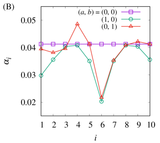
Figure 4: Ring network of ten nodes with or without a shortcut. (A) Schematic of the network . (B) Disturbance coefficients for three cases: (i) $(a,b)=(0,0)$, (ii) $(a,b)=(1,0)$, and (iii) $(a,b)=(0,1)$.

We consider the effect of a shortcut connection added to a network with a large path length. As depicted in Fig. 4(A), we consider a ring network of ten nodes, where $A_{i,i+1}=A_{i,i-1}=1$ ($1\leq i\leq N$), $A_{1,N}=A_{N,1}=1$, $A_{6,1}=a,A_{6,4}=b$, and $A_{i,j}=0$ otherwise. We compare three cases: (i) $(a,b)=(0,0)$, (ii) $(a,b)=(1,0)$, and (iii) $(a,b)=(0,1)$. Figure 4(b) shows the disturbance coefficients $\alpha_{i}$ for the three cases. When $\eta_{i}=\eta$ ($1\leq i\leq 10$), the corresponding $Q$ values are $Q^{\rm(i)}\simeq 0.413\eta,Q^{\rm(ii)}\simeq 0.354\eta$, and $Q^{\rm(iii)}\simeq 0.388\eta$. We thus find that the addition of a shortcut connection significantly improves the noise stability in both cases (ii) and (iii), with better improvement being obtained in case (ii) than in case (iii). We attribute the reason for this difference to the path length. When the path length between a pair of nodes is large, the phase difference between those nodes tends to be large. The shortcut connection in network (ii) decreases the average path length more than that of network (iii), resulting in better synchronization.

Moreover, in both, cases (ii) and (iii), node 6 gets one more incoming edge. As shown in Fig. 4(B), this reduces the disturbance coefficient of node 6 considerably. Thus, when an oscillator is very noisy, its negative effect on synchronization can be easily suppressed by adding one incoming link to the oscillator.

III.5 A ring with frequency heterogeneity

We investigate the effect of frequency heterogeneity using the ring network consisting of ten oscillators, i.e., Fig. 4(A) with $a=b=0$. We consider the case in which only one oscillator has a frequency different from the others; i.e., $\omega_{i}=\omega$ for all $i$ except $\omega_{6}=\omega+\Delta\omega$, where $\omega$ is arbitrary. For this case, network Laplacian is calculated using Eq. (24), where $(B_{ij})$ is the adjacency matrix for the ring network. We assumed $f_{ij}(\cdot)=\sin(\cdot)$ and obtained $\psi_{i}^{*}$ values ($1\leq i\leq N$) by simulating Eq. (22) in the absence of noise. Figure 5 shows the disturbance coefficients calculated numerically using Eq. (19b), indicating that the oscillators closer to node 6 more strongly disturb synchronization.

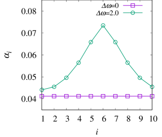
Figure 5: Disturbance coefficients $\alpha_{i}$ of the ring network of ten nodes with or without frequency heterogeneity. The natural frequencies are $\omega_{i}=\omega$ for all $i$ except $\omega_{6}=\omega+\Delta\omega$, where $\omega$ is arbitrary.

III.6 A random directed network

As a final example, we consider a random directed network of 100 oscillators. We employed a directed Erdős-Rényi model to generate $A$; i.e., $A_{ij}=1$ with probability $p$ and $A_{ij}=0$ otherwise for $j\neq i$; and $A_{ii}=0$. We set $p=0.05$, thus the mean in- and out-degrees were approximately five in our example network. We confirmed that the generated network suffices the stability criterion given in Eq. (18) and the corresponding Laplacian is diagonalizable. Figure 6(A) shows the values of the disturbance coefficients $\alpha_{i}$ obtained numerically using Eq. (19b). To see the relation between the values of $\alpha_{i}$ and the network structure, we display two scatter plots: $\alpha_{i}$ vs $1/d^{\rm in}_{i}$ in Fig. 6(B) and $\alpha_{i}$ vs $d^{\rm out}_{i}/d^{\rm in}_{i}$ in Fig. 6(C), where $d^{\rm in}_{i}$ and $d^{\rm out}_{i}$ are the in- and out-degrees of node $i$, respectively. We find that $1/d^{\rm in}_{i}$ is almost proportional to $\alpha_{i}$ and is clearly more correlated with $\alpha_{i}$ than $d^{\rm out}_{i}/d^{\rm in}_{i}$. We discuss this result later.

Figure 6: A random directed network of 100 oscillators. (A) Values of the disturbance coefficients $\alpha_{i}$. (B) $\alpha_{i}$ vs $1/d^{\rm in}_{i}$. (C) $\alpha_{i}$ vs $d^{\rm out}_{i}/d^{\rm in}_{i}$. Dashed lines are for the guidance to eye, with slopes 0.0055 and 0.001 in (B) and (C), respectively.

IV Numerical verification

Using the example network shown in Fig. 3(B), we have verified our theory numerically. We simulated Eq. (1) numerically with $f(\cdot)=\sin(\cdot)$ using random initial conditions, and we measured the Kuramoto order parameter $r(t)=\frac{1}{N}\left|\sum_{j=1}^{N}e^{i\phi_{j}}\right|$. The long-time average of $r(t)$, denoted by $R$, is expected to provide a good approximation to $\langle r\rangle$. In our simulations, we measured

$$R=\frac{1}{t_{1}-t_{0}}\int_{t_{0}}^{t_{1}}r(t)dt,$$ (36)

where $t_{0}=1000$ and $t_{1}=10000$. Furthermore, from Eqs. (9) and (19), it follows that $Q=\sum_{i}\alpha_{i}\eta_{i}=2(1-\langle r\rangle)$. Thus, by setting $(\eta_{1},\eta_{2},\eta_{3})=(\eta,0,0),(0,\eta,0)$, or $(0,0,\eta)$, we expect the quantity $2(1-R)/\eta$ to coincide with $\alpha_{i}$ $(i=1,2,3)$, respectively. In Fig. 7(a), we plot the values of $2(1-R)/\eta$ for different values of $\eta$. For small $\eta$, the numerical data are in excellent agreement with the theoretically predicted $\alpha_{i}$ values. However, for large $\eta$, there are considerable deviations, which are due to the nonlinear effects in our model.

As mentioned earlier, the network shown in Fig. 3(B) for $p=0$ yields a non-diagonalizable Laplacian $L$. We have measured the values of $2(1-R)/\eta$ numerically for different $p$ values, as shown in Fig. 7(B). The numerical values of $2(1-R)/\eta$ are in excellent agreement with the theoretical values of the $\alpha_{i}$, even for $p=0$, at which point $L$ becomes non-diagonalizable. This result supports the validity of the method proposed for treating non-diagonalizable matrices $L$ in Sec. II.3.

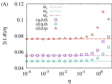
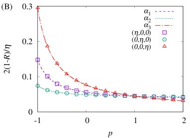
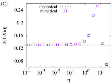
Figure 7: Numerical verification with example networks. (A) Values of $2(1-R)/\eta$ for different noise strengths $\eta$ for the network in Fig. 3 with $p=0$. (B) Values of $2(1-R)/\eta$ for the network in Fig. 3 with different $p$ values, where $\eta=0.01$. (C) Values of $2(1-R)/\eta$ for the directed random network used in III.6. Here, $R$ is the long-time-averaged Kuramoto order parameter, which is obtained from the numerical simulations of Eq. (1). The numerical values are in excellent agreement with theoretical predictions.

We then performed numerical simulation of Eq. (1) for the directed random network employed in III.6 with homogeneous noise strength $\eta_{i}=\eta$. In this case, $Q=\sum_{i}\alpha_{i}\eta\simeq 12.9\eta$. As shown in Fig. 7(C), simulation data and the predicted $Q$ value are in excellent agreement for small $\eta$.

V Discussion and conclusions

We have provided a theoretical framework for quantifying the magnitude $Q$ of the fluctuations around the synchronous state of a given oscillator network. We have also provided several example networks to discuss the optimal or better network structures. Given a nonlinear dynamical system or a network Laplacian, its $Q$ value is readily computable. Using these $Q$ values, we can quantitatively compare the noise stability of the networks of different numbers of nodes and edges with possibly heterogeneous, signed weights. Furthermore, the disturbance coefficients $\alpha_{i}$, which appear in the expression for $Q$, represent how strongly an oscillator at node $i$ disturbs synchronization. Using the values of $Q$ and $\alpha_{i}$, we can find the optimal network structure and the optimal oscillator configuration, as demonstrated in Sec. III.

In the example shown in Fig. 4, we show that shortcut connections are effective for making oscillator networks noise-tolerant. Such networks are often referred to as small-world networks Watts and Strogatz (1998), and there is a large body of theoretical results indicating that synchronization is enhanced as the number of shortcuts increases. Among them, the study by Korniss et al. Korniss et al. (2003) is very relevant to the present study. They employed a course-grained description of the oscillator network to show that shortcut connections added to lattice networks prevent the divergence of the phase variance, given in Eq. (19a), as $N$ goes infinity Korniss et al. (2003). Such an approach is certainly powerful for understanding typical properties shared by certain network classes. Our approach can be regarded as a complementary one. We can quantify fluctuations in synchronized dynamics in particular networks of any class in a detailed manner.

Our study is based on a general class of linear dynamical systems with additive noise, given in Eq. (12). There are other theoretical studies concerning the same linear systems that treat different quantities of interest. For example, Refs. Kori et al. (2009); Masuda, Kawamura, and Kori (2010); Cross (2012) investigate the dynamics of the collective mode of an oscillator network. This problem can concisely be formulated as a projection of the entire dynamical system onto a one-dimensional dynamical mode along the synchronization manifold, which is $\bm{u}^{(1)}$ in the present theory. For example, when oscillators are subjected to independent noise, as we consider in the present paper, the diffusion coefficient of the collective mode can be derived as a function of $\bm{v}^{(1)}$ Masuda, Kawamura, and Kori (2010). Moreover, it has been shown that element $w_{i}$ of $\bm{v}^{(1)}=(w_{1}\,w_{2}\,\ldots\,w_{N})$ describes the strength of the influence of node $i$ on the collective mode Kori et al. (2009); Masuda, Kawamura, and Kori (2009a); Skardal et al. (2016).

We emphasize that $w_{i}$ and $\alpha_{i}$ are different measures because they are related to the dynamics along and transverse to the synchronization manifold, respectively. Therefore, they are not necessarily correlated. For example, for symmetric $L$, $w_{i}$ is constant for all nodes whereas $\alpha_{i}$ can be heterogeneous. Actually, as shown in Fig. 5, $\alpha_{i}$ is heterogeneous for $\Delta\omega=2.0$ in spite of symmetric $L$. However, in large directed random networks, they seem to be positively correlated because $w_{i}$ is roughly proportional to $d^{\rm out}_{i}/d^{\rm in}_{i}$, which is derived using a mean-field approximation Masuda, Kawamura, and Kori (2009b), whereas $\alpha_{i}$ is approximately proportional to $1/d^{\rm in}_{i}$ as is numerically found in Fig. 6(B). Namely, a node with a small incoming degree tends to have large $w_{i}$ and $\alpha_{i}$ values. The property $\alpha_{i}\sim 1/d^{\rm in}_{i}$ is not theoretically rationalized and remains an important open problem. However, it makes sense that $\alpha_{i}$ tends to be larger for smaller $d^{\rm in}_{i}$ because such nodes can only weakly tune their own rhythm to others and thus more strongly disturb the population.

Ref. Kori, Kawamura, and Masuda (2012) treats the precision of the cycle-to-cycle periods of a synchronous state in an oscillator network. This problem involves all the dynamical modes, as is also the case for the present problem. However, the major contribution to the fluctuations in cycle-to-cycle periods comes from the dynamical mode along the synchronization manifold; in contrast, our problem is independent of such a mode. This is the reason why the contribution of the zero eigenmode is absent from our expression for $Q$; i.e., the summation in Eq. (19a) starts from $m,n=2$.

Many studies on the stability of synchronization focus on a few eigenmodes, such as the mode associated with $\lambda_{2}$ because it characterizes the long-time behavior of the relaxation process to a synchronized state in the absence of noise. In contrast, when noise is present, noise keeps to excite all the eigenmodes. Noise stability is thus involved with all the eigenmodes, as reflected in the expressions for $Q$ and $\alpha_{i}$. When a part of eigenvalues have vanishingly small real parts, the contributions of other eigenmodes can be neglected in those expressions. However, such a situation is exceptional, such as when the system is near the synchronization-desynchronization transition point.

Synchronization is essential in various artistic performances, including those of orchestras, choruses, and dancers. To improve synchronization in such performances, our theory may be helpful in indicating a better network structure, the placement of experts and laymen, and who to have look at whom. Experimental study, such as synchronization continuation of finger tapping Okano, Shinya, and Kudo (2017), is required to demonstrate our theoretical study.

Appendix A Derivation of Eq. (19)

We decompose $\bm{x}$ as

$$\bm{x}(t)=\sum_{m=1}^{N}y_{m}(t)\bm{u}^{(m)},$$ (37)

where $y_{m}(t)$ is given by

$$y_{m}(t)={\bm{v}}^{(m)}\bm{x}(t).$$ (38)

By taking the time derivative of Eq. (38) and using Eqs. (11) and (15), we obtain

$$\dot{y}_{m}(t)=-\lambda_{m}y_{m}(t)+\hat{\xi}_{m}(t),$$ (39)

where

$$\hat{\xi}_{m}(t)=\sum_{i=1}^{N}v_{i}^{(m)}\xi_{i}(t).$$ (40)

It is straightforward to show that

$$\langle\hat{\xi}_{m}(t)\rangle=0,\quad\langle\hat{\xi}_{m}(t)\hat{\xi}_{n}(s)\rangle=\hat{\eta}_{mn}\delta(t-s),$$ (41)

where

$$\hat{\eta}_{mn}=\sum_{i=1}^{N}v_{i}^{(m)}v_{i}^{(n)}\eta_{i}.$$ (42)

The solution to Eq. (39) can be formally written as

$$y_{m}(t)=e^{-\lambda_{m}t}y_{m}(0)+\int_{0}^{t}e^{-\lambda_{m}(t-s)}\hat{\xi}_{m}(s)ds.$$ (43)

For $m,n\geq 2$, using Eqs. (41) and (43), we obtain

$$\left\langle y_{m}(t)y_{n}(t)\right\rangle$$

$$=\left\langle\left(e^{-\lambda_{m}t}y_{m}(0)+\int_{0}^{t}e^{-\lambda_{m}(t-s_{1})}\hat{\xi}_{m}(s_{1})ds_{1}\right)\left(e^{-\lambda_{n}t}y_{n}(0)+\int_{0}^{t}e^{-\lambda_{n}(t-s_{2})}\hat{\xi}_{n}(s_{2})ds_{2}\right)\right\rangle$$ (44)

$$=\left\langle e^{-\lambda_{m}t}y_{m}(0)e^{-\lambda_{n}t}y_{n}(0)\right\rangle+\left\langle e^{-\lambda_{m}t}y_{m}(0)\int_{0}^{t}e^{-\lambda_{n}(t-s_{2})}\hat{\xi}_{n}(s_{2})ds_{2}\right\rangle+\left\langle e^{-\lambda_{n}t}y_{n}(0)\int_{0}^{t}e^{-\lambda_{m}(t-s_{1})}\hat{\xi}_{m}(s_{1})ds_{1}\right\rangle$$

$$\qquad+\left\langle\int_{0}^{t}e^{-\lambda_{m}(t-s_{1})}\hat{\xi}_{m}(s_{1})ds_{1}\int_{0}^{t}e^{-\lambda_{n}(t-s_{2})}\hat{\xi}_{n}(s_{2})ds_{2}\right\rangle$$ (45)

$$=e^{-(\lambda_{m}+\lambda_{n})t}y_{m}(0)y_{n}(0)+\left\langle\int_{0}^{t}ds_{1}\int_{0}^{t}ds_{2}e^{-\lambda_{m}(t-s_{1})}\hat{\xi}_{m}(s_{1})e^{-\lambda_{n}(t-s_{2})}\hat{\xi}_{n}(s_{2})\right\rangle$$ (46)

$$=e^{-(\lambda_{m}+\lambda_{n})t}y_{m}(0)y_{n}(0)+\int_{0}^{t}ds_{1}\int_{0}^{t}ds_{2}e^{-\lambda_{m}(t-s_{1})}e^{-\lambda_{n}(t-s_{2})}\left\langle\hat{\xi}_{m}(s_{1})\hat{\xi}_{n}(s_{2})\right\rangle$$ (47)

$$=e^{-(\lambda_{m}+\lambda_{n})t}y_{m}(0)y_{n}(0)+\int_{0}^{t}ds_{1}\int_{0}^{t}ds_{2}e^{-\lambda_{m}(t-s_{1})}e^{-\lambda_{n}(t-s_{2})}\hat{\eta}_{mn}\delta(s_{1}-s_{2})$$ (48)

$$=e^{-(\lambda_{m}+\lambda_{n})t}y_{m}(0)y_{n}(0)+\hat{\eta}_{mn}\int_{0}^{t}dse^{-(\lambda_{m}+\lambda_{n})(t-s)}$$ (49)

$$=e^{-(\lambda_{m}+\lambda_{n})t}y_{m}(0)y_{n}(0)+\hat{\eta}_{mn}\frac{1-e^{-(\lambda_{m}+\lambda_{n})t}}{\lambda_{m}+\lambda_{n}}$$ (50)

$$\to\frac{\hat{\eta}_{mn}}{\lambda_{m}+\lambda_{n}}\quad(t\to\infty)$$ (51)

Here, we take the limit $t\to\infty$ because we are interested in a steady process in which the dependence on initial conditions vanishes.

Now we derive the expression for $Q$. For convenience, we rewrite the definitions:

$$\overline{x}=\frac{1}{N}\sum_{j=1}^{N}x_{i},$$ (52)

$$\overline{u^{(m)}}=\frac{1}{N}\sum_{j=1}^{N}u_{j}^{(m)},$$ (53)

$$\overline{u^{(m)}u^{(n)}}=\frac{1}{N}\sum_{j=1}^{N}u_{j}^{(m)}u_{j}^{(n)}$$ (54)

Using Eq. (37), i.e., $x_{j}=\sum_{m=1}^{N}u_{j}^{(m)}y_{m}$, we obtain

$$Q =\frac{1}{N}\sum_{j=1}^{N}\left\langle(x_{j}-\overline{x})^{2}\right\rangle$$ (55)

$$=\frac{1}{N}\sum_{j=1}^{N}\left\langle\left(\sum_{m=1}^{N}\left(u_{j}^{(m)}-\overline{u^{(m)}}\right)y_{m}\right)\left(\sum_{n=1}^{N}\left(u_{j}^{(n)}-\overline{u^{(n)}}\right)y_{n}\right)\right\rangle$$

$$=\frac{1}{N}\sum_{j=1}^{N}\sum_{m,n=1}^{N}\left(u_{j}^{(m)}u_{j}^{(n)}-u_{j}^{(m)}\overline{u^{(n)}}-\overline{u^{(m)}}u_{j}^{(n)}+\overline{u^{(m)}}\ \overline{u^{(n)}}\right)\left\langle y_{m}(t)y_{n}(t)\right\rangle.$$ (56)

$$=\sum_{m,n=1}^{N}\left(\overline{u^{(m)}u^{(n)}}-\overline{u^{(m)}}\ \overline{u^{(n)}}\right)\left\langle y_{m}(t)y_{n}(t)\right\rangle$$ (57)

$$=\sum_{m,n=2}^{N}\left(\overline{u^{(m)}u^{(n)}}-\overline{u^{(m)}}\ \overline{u^{(n)}}\right)\left\langle y_{m}(t)y_{n}(t)\right\rangle$$ (58)

$$=\sum_{m,n=2}^{N}\left(\overline{u^{(m)}u^{(n)}}-\overline{u^{(m)}}\ \overline{u^{(n)}}\right)\frac{\hat{\eta}_{mn}}{\lambda_{m}+\lambda_{n}},$$ (59)

$$=\sum_{m,n=2}^{N}\left(\overline{u^{(m)}u^{(n)}}-\overline{u^{(m)}}\ \overline{u^{(n)}}\right)\frac{\hat{\eta}_{mn}}{\lambda_{m}+\lambda_{n}},$$ (60)

$$=\sum_{i=1}^{N}\sum_{m,n=2}^{N}\frac{\overline{u^{(m)}u^{(n)}}-\overline{u^{(m)}}\ \overline{u^{(n)}}}{\lambda_{m}+\lambda_{n}}{v_{i}^{(m)}v_{i}^{(n)}}\eta_{i},$$ (61)

which is Eq. (19). To pass from Eq. (57) to Eq. (58), we have used the relation

$$\overline{u^{(m)}u^{(n)}}-\overline{u^{(m)}}\ \overline{u^{(n)}}=0\quad\mbox{for $m=1$ or $n=1$},$$ (62)

which holds because $\bm{u}^{(1)}=(1,1,\ldots,1)^{\rm T}$.

For a symmetric matrix $L$, Eq. (19b) reduces to Eq. (20) because $\bm{v}^{(n)}=(\bm{u}^{(n)})^{\mathrm{T}}$, $\bm{u}^{(m)}\cdot\bm{u}^{(n)}=\delta_{mn}$ for $1\leq m,n\leq N$, $\overline{u^{(n)}}=\frac{1}{N}\sum_{i=1}^{N}u_{i}^{(n)}\propto\sum_{i=1}^{N}u_{i}^{(1)}u_{i}^{(n)}=\bm{u}^{(1)}\cdot\bm{u}^{(n)}=0$, and $\overline{u^{(m)}u^{(n)}}=\frac{1}{N}\,\bm{u}^{(m)}\cdot\bm{u}^{(n)}=\frac{\delta_{mn}}{N}$.

References

- Winfree (2001) A. T. Winfree, The geometry of biological time (Springer-Verlag New York, 2001).
- Kuramoto (1984) Y. Kuramoto, Chemical Oscillations, Waves, and Turbulence (Springer-Verlag Berlin Heidelberg, 1984).
- Pikovsky, Rosenblum, and Kurths (2001) A. Pikovsky, M. Rosenblum, and J. Kurths, Synchronization: a universal concept in nonlinear sciences (Cambridge University Press, 2001).
- Glass (2001) L. Glass, “Synchronization and rhythmic processes in physiology,” Nature 410, 277–284 (2001).
- Hoyt and Taylor (1981) D. F. Hoyt and C. R. Taylor, “Gait and the energetics of locomotion in horses,” Nature 292, 239 (1981).
- Taga, Yamaguchi, and Shimizu (1991) G. Taga, Y. Yamaguchi, and H. Shimizu, “Self-organized control of bipedal locomotion by neural oscillators in unpredictable environment,” Biological cybernetics 65, 147–159 (1991).
- Ijspeert (2008) A. J. Ijspeert, “Central pattern generators for locomotion control in animals and robots: a review,” Neural networks 21, 642–653 (2008).
- Stoklasa, Liebermann, and Fischinger (2012) J. Stoklasa, C. Liebermann, and T. Fischinger, “Timing and synchronization of professional musicians: a comparison between orchestral brass and string players,” in 12th international conference on music perception and cognition, Thessaloniki, Greece (2012).
- Miyashita et al. (2011) Y. Miyashita, Y. Ishibashi, N. Fukushima, S. Sugawara, and K. E. Psannis, “Qoe assessment of group synchronization in networked chorus with voice and video,” in TENCON 2011-2011 IEEE Region 10 Conference (IEEE, 2011) pp. 192–196.
- Wuyts and Buekers (1995) I. J. Wuyts and M. J. Buekers, “The effects of visual and auditory models on the learning of a rhythmical synchronization dance skill,” Research quarterly for exercise and sport 66, 105–115 (1995).
- Elowitz et al. (2002) M. B. Elowitz, A. J. Levine, E. D. Siggia, and P. S. Swain, “Stochastic gene expression in a single cell,” Science 297, 1183–1186 (2002).
- Faisal, Selen, and Wolpert (2008) A. A. Faisal, L. P. Selen, and D. M. Wolpert, “Noise in the nervous system,” Nature reviews neuroscience 9, 292 (2008).
- Arenas et al. (2008) A. Arenas, A. Díaz-Guilera, J. Kurths, Y. Moreno, and C. Zhou, “Synchronization in complex networks,” Physics reports 469, 93–153 (2008).
- Masuda, Porter, and Lambiotte (2017) N. Masuda, M. A. Porter, and R. Lambiotte, “Random walks and diffusion on networks,” Physics Reports (2017).
- Olfati-Saber, Fax, and Murray (2007) R. Olfati-Saber, J. A. Fax, and R. M. Murray, “Consensus and cooperation in networked multi-agent systems,” Proc. IEEE 95, 215–233 (2007).
- Nakao and Mikhailov (2010) H. Nakao and A. S. Mikhailov, “Turing patterns in network-organized activator–inhibitor systems,” Nature Physics 6, 544 (2010).
- Mohar et al. (1991) B. Mohar, Y. Alavi, G. Chartrand, and O. Oellermann, “The laplacian spectrum of graphs,” Graph theory, combinatorics, and applications 2, 12 (1991).
- Chung (1997) F. R. Chung, Spectral graph theory (American Mathematical Soc., 1997).
- Barahona and Pecora (2002) M. Barahona and L. M. Pecora, “Synchronization in small-world systems,” Phys. Rev. Lett. 89, 054101 (2002).
- Nishikawa and Motter (2006) T. Nishikawa and A. E. Motter, “Synchronization is optimal in nondiagonalizable networks,” Phys. Rev. E 73, 065106 (2006).
- Winfree (1967) A. T. Winfree, “Biological rhythms and the behavior of populations of coupled oscillators,” Journal of theoretical biology 16, 15–42 (1967).
- Kopell and Ermentrout (2004) N. Kopell and B. Ermentrout, “Chemical and electrical synapses perform complementary roles in the synchronization of interneuronal networks,” Proc. Nat. Acad. Sci. USA 101, 15482–15487 (2004).
- Kiss, Zhai, and Hudson (2005) I. Z. Kiss, Y. Zhai, and J. L. Hudson, “Predicting mutual entrainment of oscillators with experiment-based phase models,” Phys. Rev. Lett. 94, 248301 (2005).
- Miyazaki and Kinoshita (2006) J. Miyazaki and S. Kinoshita, “Determination of a coupling function in multicoupled oscillators,” Phys. Rev. Lett. 96, 194101 (2006).
- Kori et al. (2014) H. Kori, Y. Kuramoto, S. Jain, I. Z. Kiss, and J. L. Hudson, “Clustering in globally coupled oscillators near a hopf bifurcation: theory and experiments,” Phys. Rev. E 89, 062906 (2014).
- Stankovski et al. (2017) T. Stankovski, T. Pereira, P. V. McClintock, and A. Stefanovska, “Coupling functions: universal insights into dynamical interaction mechanisms,” Rev. Mod. Phys. 89, 045001 (2017).
- Risken (1996) H. Risken, The Fokker-Planck Equation (Springer, 1996).
- Ermentrout (1992) G. B. Ermentrout, “Stable periodic solutions to discrete and continuum arrays of weakly coupled nonlinear oscillators,” SIAM Journal on Applied Mathematics 52, 1665–1687 (1992).
- Yanagita and Ichinomiya (2014) T. Yanagita and T. Ichinomiya, “Thermodynamic characterization of synchronization-optimized oscillator networks,” Phys. Rev. E 90, 062914 (2014).
- Masuda, Kawamura, and Kori (2010) N. Masuda, Y. Kawamura, and H. Kori, “Collective fluctuations in networks of noisy components,” New Journal of Physics 12, 093007 (2010).
- Milo et al. (2002) R. Milo, S. Shen-Orr, S. Itzkovitz, N. Kashtan, D. Chklovskii, and U. Alon, “Network motifs: simple building blocks of complex networks,” Science 298, 824–827 (2002).
- Watts and Strogatz (1998) D. J. Watts and S. H. Strogatz, “Collective dynamics of ‘small-world’ networks,” nature 393, 440 (1998).
- Korniss et al. (2003) G. Korniss, M. Novotny, H. Guclu, Z. Toroczkai, and P. A. Rikvold, “Suppressing roughness of virtual times in parallel discrete-event simulations,” Science 299, 677–679 (2003).
- Kori et al. (2009) H. Kori, Y. Kawamura, H. Nakao, K. Arai, and Y. Kuramoto, “Collective-phase description of coupled oscillators with general network structure,” Phys. Rev. E 80, 036207 (2009).
- Cross (2012) M. Cross, “Improving the frequency precision of oscillators by synchronization,” Phys. Rev. E 85, 046214 (2012).
- Masuda, Kawamura, and Kori (2009a) N. Masuda, Y. Kawamura, and H. Kori, “Analysis of relative influence of nodes in directed networks,” Phys. Rev. E 80, 046114 (2009a).
- Skardal et al. (2016) P. S. Skardal, D. Taylor, J. Sun, and A. Arenas, “Collective frequency variation in network synchronization and reverse pagerank,” Phys. Rev. E 93, 042314 (2016).
- Masuda, Kawamura, and Kori (2009b) N. Masuda, Y. Kawamura, and H. Kori, “Impact of hierarchical modular structure on ranking of individual nodes in directed networks,” New J. Phys. 11, 113002 (2009b).
- Kori, Kawamura, and Masuda (2012) H. Kori, Y. Kawamura, and N. Masuda, “Structure of cell networks critically determines oscillation regularity,” Journal of Theoretical Biology 297, 61–72 (2012).
- Okano, Shinya, and Kudo (2017) M. Okano, M. Shinya, and K. Kudo, “Paired synchronous rhythmic finger tapping without an external timing cue shows greater speed increases relative to those for solo tapping,” Scientific Reports 7, 43987 (2017).