True Nonlinear Dynamics from Incomplete Networks

Abstract

We study nonlinear dynamics on complex networks. Each vertex $i$ has a state $x_{i}$ which evolves according to a networked dynamics to a steady-state $x_{i}^{*}$. We develop fundamental tools to learn the true steady-state of a small part of the network, without knowing the full network. A naive approach and the current state-of-the-art is to follow the dynamics of the observed partial network to local equilibrium. This dramatically fails to extract the true steady state. We use a mean-field approach to map the dynamics of the unseen part of the network to a single node, which allows us to recover accurate estimates of steady-state on as few as 5 observed vertices in domains ranging from ecology to social networks to gene regulation. Incomplete networks are the norm in practice, and we offer new ways to think about nonlinear dynamics when only sparse information is available.

1 Dynamical Systems on Incomplete Networks

The fundamental task in learning is to infer unknown quantities of interest from incomplete data. We study learning complex nonlinear dynamics on networks from incomplete data. Such problems are fundamental because complex nonlinear dynamical systems are ubiquitous, often modeled as coupled nonlinear ordinary differential equations (ODEs), for example epidemic spreading (?), Michaelis-Menten gene regulatory dynamics (?; ?), Lotka-Volterra ecological dynamics (?). A graph $G=(V,E)$ with $n\times n$ (weighted) adjacency matrix $A$ is the backbone on which the dynamical equations are coupled together. We consider a general dynamics in which each vertex $i$ of $G$ has a state $x_{i}$ which evolves according to a self-driving force and a sum of interaction forces over neighbors

$$\dot{x}_{i}=f(x_{i})+\sum_{j\in V}A_{ij}g(x_{i},x_{j}).$$ (1)

The functions $f(\cdot)$ and $g(\cdot,\cdot)$ are general and usually nonlinear, and the positive weighted connectivity matrix $A$ modulates the interactions between vertices. Several instances of such dynamics with appropriate choices of $f(\cdot)$ and $g(\cdot,\cdot)$ are shown in Table 1. From an initial state, one can step forward in time, simulating the dynamics in (1) until convergence to equilibrium states $x_{i}^{*}$.

The complete information setting in (1) is unrealistic, and we must accept that in practice, only part of a network can be measured. Hence, we assume that a subgraph with $m$ nodes $G^{(s)}=(V^{(s)},E^{(s)})$ is known, with corresponding $m\times m$ adjacency matrix $A^{(s)}$, where $V^{(s)}\subseteq V$ and $E^{(s)}\subseteq E$ ($s$ for sampled). This paradigm is unavoidable when the full network is unmeasurable (for example, protein-protein interactions, metabolic and terrorist networks (?)). The paradigm is also useful when the full network is too large to handle, where one can deliberately sample a much smaller subnetwork for the analysis. Analyzing a full network from a sampled subnetwork has been studied in several contexts, e.g. to estimate average or total degree (?); degree distributions and clustering coefficients (?; ?; ?); shortest paths (?); motif counts (?); vertex and edge counts (?; ?).

Applications	Vertex	State at vertex $i$	Dynamics
Ecological ( ?; ? )	Species	Abundance	$\dot{x}_{i}=B_{i}+x_{i}(1-\frac{x_{i}}{K_{i}})(\frac{x_{i}}{C_{i}}-1)+\sum_{j}A_{ij}\frac{x_{i}x_{j}}{D_{i}+E_{i}x_{i}+H_{j}x_{j}}$
Regulatory ( ?; ? )	Gene	Expression level	$\dot{x}_{i}=-Bx_{i}^{f}+\sum_{j}A_{ij}R\frac{x_{j}^{h}}{x_{j}^{h}+1}$
Epidemic ( ?; ?; ? )	Person	Infection rate	$\dot{x}_{i}=-Bx_{i}+\sum_{j}A_{ij}R(1-x_{i})x_{j}$

Table 1: Examples of real systems with nonlinear interaction dynamics.

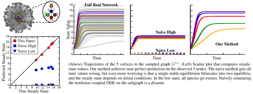
Figure 1: Predicting steady-state abundances of 5 species interacting in a larger 97 species ecological network. Predictions use only the interactions of those five species (incomplete information).

Our task is to estimate true steady-states $x^{*}$ for vertices in $V^{(s)}$, despite only seeing an incomplete network $G^{(s)}$. The state-of-the-art naive approach is to simulate (1) on the subgraph $G^{(s)}$. For example, one may collect a social network from Boston and run the epidemic model (Table 1) to obtain the probability of each person to be infected. The results are a dramatic and universal disaster, because the sub-social network of Boston is just a small part of a vast social network, and the people in Boston interact with people outside. That the naive method is bad is not surprising because the essence of the dynamics in (1) are the interactions, and the subgraph is missing many of those interactions. Hence, not observing a large part of the network appears to be an insurmountable hurdle to learning the true steady states on the observed (small) part of the network.

We develop a methodology to accurately predict true steady states using only information local to $G^{(s)}$. We demonstrate the power of our approach in Figure 1, for an ecological network where vertices are species and states are species-abundance. This ecological network of 97 species follows the symbiotic dynamics in Table 1, see (?). Let us see what happens when a biologist who is interested in five species collects the relevant 5-vertex subgraph $G^{(s)}$ and performs a naive simulation on the subgraph to get a steady-state. The results in Figure 1 are as expected. The naive simulation is wrong. Even worse, it cannot identify the number of equilibria from the subgraph: the full network has one attractor, but the subgraph has two. It means that, with the wrong initial conditions, the biologist would conclude that the five species are going extinct, when in fact they are all doing fine in the real network.

Our Contributions. We give the first method to accurately learn steady-state dynamics when only a part of the network is observed. This is remarkable given the inherent interactive nature of the dynamics. The result in Figure 1 demonstrates that our methods extract very close approximations to the true steady state dynamics in the full network when just 5% of vertices are observed. This surprising result has the potential for huge impact since up to now, the state-of-the-art is the naive approach which produces completely wrong conclusions. There are three main ideas behind our method.

• A mean field approximation to account for the impact of the unobserved part of the network.

• Summarizing the mean field impact using a resilience parameter, $\beta$, which depends only on network topology. How the resilience impacts the final outcome depends on the coupled nonlinear dynamics through $f(\cdot)$ and $g(\cdot,\cdot)$.

• Estimating the full network’s resilience from the observed subgraph. A network’s resilience is important in other contexts. The resilience characterizes a complex system’s ability to retain its basic functionality under edge and vertex faults. Hence, our estimates of resilience from incomplete information are of independent interest.

Combining these three ideas, we obtain accurate estimates of the steady-states as in Figure 1. Our estimates are near-exact matches to the true steady-states.

2 Model

The true dynamics on the full network $G$ are governed by the coupled nonlinear dynamics in (1). We represent $G$ by its adjacency matrix $A$, and assume that the total size of the network, $n$, is known. The observed sampled subgraph $G^{(s)}=(V^{(s)},E^{(s)})$ has adjacency matrix $A^{(s)}$. There are many ways to sample vertices and edges from a graph. We focus on two natural sampling methods which are reasonable models of how the incomplete data is often obtained.

• (Random Vertex Sampling) Form the induced subgraph for randomly sampled vertices. We assume the degrees of the sampled vertices are also known. For example, we know the number of friends each person has in a social network and who is friends with whom among the sampled subnetwork.

• (Random Walk) A random vertex is sampled. At each step, an available edge is followed to sample a new vertex. The degrees of the vertices are implicitly available since, at each step, the available edges must be known.

Our method can be extended to other sampling schemes, such as edge sampling, degree biased sampling, Metropolis-Hastings random walks. The main property we require of the sampling is that specific topological parameters of the graph can be reliably estimated from the sample.

For $i\in V^{(s)}$, the steady-state value in $G$ is denoted $x_{i}^{*}$. We denote by $z_{i}^{*}$ the steady-state value obtained using the partially observed network. We loosely use $z_{i}$ to refer both to the vertex and state variable at the vertex. The naive method solves the same system in (1) for $A^{(s)}$ instead of $A$. That is, for $i\in V^{(s)}$, $z_{i}^{*}$ is the steady-state of the dynamical system

$$\text{(Naive method)}~{}~{}~{}~{}~{}~{}\dot{z}_{i}=f(z_{i})+\sum_{j\in V^{(s)}}A^{(s)}_{ij}g(z_{i},z_{j}).$$ (2)

This naive approach produces incorrect conclusions, yet it is common practice because that’s all practitioners have. To get correct results, one must account for missing data.

3 Mean Field Approximation and Resilience

The main idea is shown in the (sampled) subgraph in Figure 2(a). We focus on one vertex in $V^{(s)}$, $z_{2}$. Vertex $z_{2}$ interacts with its neighbors $z_{1}$ and $z_{4}$ in the subgraph, and its neighbors outside the subgraph. All the subgraph nodes $z_{1},\ldots,z_{5}$ are in a similar situation. Now fix the value for each external neighbor of $z_{2}$ to its true steady-state value in the full network, shown as $x_{1}^{*},x_{2}^{*},x_{3}^{*}$. Do the same for the external neighbors of all the subgraph vertices $z_{1},\ldots,z_{5}$. As far as the subgraph is concerned, all external neighbors have converged to their steady-state values and are providing the right interactive feedback to all subgraph nodes. The subgraph is effectively isolated from the rest of the network and will converge to steady-states of the full network. We state the next theorem without proof. The preceding discussion essentially amounts to the proof.

Figure 2: Mean field approximation.

Theorem 1.

The steady-states $z_{i}^{*}$ of the dynamical system

$$\dot{z}_{i}=f(z_{i})+\sum_{j\in V^{(s)}}A^{(s)}_{ij}g(z_{i},z_{j})+\sum_{j\not\in V^{(s)}}A_{ij}g(z_{i},x_{j}^{*})$$ (3)

recover one of the true steady-states of the full network.

We cannot implement (3), because $x_{i}^{*}$ are unknown. In the mean field approximation, we replace $x_{i}^{*}$ by an average influence $x_{\text{eff}}$, see Figure 2(b). Of course it is an approximation, but it works well for analyzing complex interacting systems such as spin-systems (?). The iteration-0 estimate is $x_{\text{eff}}$ for all states.

Fix the states for all vertices but (say) $z_{2}$ to $x_{\text{eff}}$, and find the steady-state for $z_{2}$, as in Figure 2(b). Now, $z_{2}$ is effectively isolated from the rest of the network as all its neighbors are fixed at $x_{\text{eff}}$. So, $z_{2}$ evolves to a steady-state, following the dynamics $\dot{z}_{2}=f(z_{2})+5g(z_{2},x_{\text{eff}})$. Repeat for each subgraph-vertex to arrive at $z_{i}^{(1)}$, the steady-states of

$$\dot{z}_{i}=f(z_{i})+\delta_{i}g(z_{i},x_{\text{eff}}),$$ (4)

where $\delta_{i}$ is the degree of $z_{i}$ in $G$. These equations are uncoupled since $x_{\text{eff}}$ is fixed. This is the method used in (?) to analyze the dynamics on the full network by reducing to $n$ uncoupled ODEs. We now iterate further. Suppose the steady-state from iteration $\tau$ is $z_{i}^{(\tau)}$. We obtain $z_{i}^{(\tau+1)}$, the approximation at iteration $\tau+1$ as the steady-state solution to the uncoupled equations

Comparing (5) to the exact solution in (3), the external forces are replaced by an effective external force and the interaction term is approximated by an interaction to a previous steady-state. Iterating to convergence, $z^{(\tau)}_{i}$ converges to a steady-state $z_{i}^{*}$ which solves the coupled system

where $\delta_{i}^{(s)}$ is the degree of $z_{i}$ in $G^{(s)}$.

The naive method in (2) resembles (6) with one crucial difference, an additional term for the external force on a vertex. The entire system in (6) corresponds to adding just one more vertex to our subgraph, whose value is fixed at $x_{\text{eff}}$, with a weighted edge to $z_{i}$ of weight $A^{(s)}_{i,x_{\text{eff}}}=\delta_{i}-\delta_{i}^{(s)}$. We show this augmented graph for our example in Figure 2(c).

Next, we discuss how to compute $x_{\text{eff}}$ to estimate the mean-field interaction with unseen vertices. The complication is that this estimate cannot depend on the missing information. This is possible because $x_{\text{eff}}$ depends on the missing information only through global topological statistics of the network, and we can estimate those topological statistics when the subgraph is sampled appropriately.

3.1 Computing the Effective External Impact

There are two unknown quantities in (6). The degree $\delta_{i}$ and $x_{\text{eff}}$. We now discuss $x_{\text{eff}}$, following the general approach in (?). Consider vertex $i$ and the interaction term $\sum_{j}A_{ij}g(x_{i},x_{j})$ in (1), where $A_{ij}$ is the influence $j$ has on $i$. The in-degree $s^{\text{in}}_{i}=\sum_{j}A_{ij}$ and the out-degree $s^{\text{out}}_{i}=\sum_{j}A_{ji}$. Assuming $A_{ij}\geq 0$, the interaction term is the in-degree times an average interaction,

$$\sum_{j}A_{ij}g(x_{i},x_{j})=s^{\text{in}}_{i}\frac{\sum_{j}A_{ij}g(x_{i},x_{j})}{\sum_{k}A_{ik}}$$ (7)

Here, the in-degree $s^{\text{in}}_{i}$ captures the idiosyncratic part, and the average $g(\cdot,\cdot)$ captures the network effect. Our first mean-field approximation is to replace local averaging with global averaging, which approximates the network-impact on a vertex as nearly homogeneous. Specifically, we have

where the vector $g(x_{i},\bm{x})$ has $j$th component $g(x_{i},x_{j})$. Define an averaging linear operator

$${\cal L}_{A}({\bm{z}})=\frac{\bm{1}^{T}A}{\bm{1}^{T}A\bm{1}}{\bm{z}}=\frac{\bm{s}^{\text{out}}\cdot{\bm{z}}}{\bm{s}^{\text{out}}\cdot\bm{1}},$$ (9)

which is a weighted average of the entries in $\bm{z}$. Our mean-field approximation results in the approximate dynamics

$$\dot{x}_{i}=f(x_{i})+s^{\text{in}}_{i}{\cal L}_{A}[g(x_{i},\bm{x})].$$ (10)

In the first order linear approximation, we take ${\cal L}_{A}$ inside $g$. Our second mean-field approximation is that the average of external interactions is approximately the interaction with the average. That is ${\cal L}_{A}[g(x_{i},\bm{x})]\approx g(x_{i},{\cal L}_{A}(\bm{x}))$ and

$$\dot{x}_{i}=f(x_{i})+s^{\text{in}}_{i}g(x_{i},{\cal L}_{A}(\bm{x})),$$ (11)

where ${\cal L}_{A}(\bm{x})$ is a global state. Let $x_{\text{av}}\triangleq{\cal L}_{A}(\bm{x})$. Applying ${\cal L}_{A}$ to both sides of (11) gives

$$\dot{x}_{\text{av}}={\cal L}_{A}[f(\bm{x})]+{\cal L}_{A}[\bm{s^{\text{in}}}g(\bm{x},x_{\text{av}})].$$ (12)

Extensive tests in (?) show that the in-degrees $s^{\text{in}}_{i}$ and the interactions $g(x_{i},x_{\text{av}})$ are roughly uncorrelated, so the ${\cal L}_{A}$-average of the product is the product of ${\cal L}_{A}$-averages. Thus, our third mean-field approximation is ${\cal L}_{A}[\bm{s^{\text{in}}}g(\bm{x},x_{\text{av}})]\approx{\cal L}_{A}(\bm{s^{\text{in}}}){\cal L}_{A}[g(\bm{x},x_{\text{av}})]$. Using the linear approximation again, we take the ${\cal L}_{A}$-average inside $f$ and $g$

$$\dot{x}_{\text{av}}=f({\cal L}_{A}(\bm{x}))+{\cal L}_{A}(\bm{s^{\text{in}}})g({\cal L}_{A}(\bm{x}),x_{\text{av}}).$$ (13)

Now we have a dynamical system for $x_{\text{av}}$,

$$\dot{x}_{\text{av}}=f(x_{\text{av}})+\beta g(x_{\text{av}},x_{\text{av}}),$$ (14)

where the resilience $\beta={\cal L}_{A}(\bm{s}^{\rm in})$. For undirected graphs, $\beta=\sum_{i}\delta_{i}^{2}/\sum_{i}\delta_{i}=\langle\delta^{2}\rangle/\langle\delta\rangle$. The steady-state of (14) is the external effective impact, $x_{\text{eff}}$. Plugging it into (11) gives an uncoupled ODE for $x_{i}$,

$$\dot{x}_{i}=f(x_{i})+s^{\text{in}}_{i}g(x_{i},x_{\text{eff}}).$$ (15)

In the mean-field approximation, $g(x_{i},x_{j})$ in (1) is replaced by an interaction with a mean-field external world $g(x_{i},x_{\text{eff}})$ and the number of neighbors impacting $x_{i}$ is captured by $s^{\text{in}}_{i}$. To approximately obtain the steady-states of the system, one first solves the ODE in (14) to get $x_{\text{eff}}$, and then $n$ uncoupled ODEs at each vertex to get $x_{i}$, which only depends on $s^{\text{in}}_{i}$ if given $x_{\text{eff}}$. The method works well because the mean-field approximations only need to hold at the steady-state. Hence, we can recover the steady-state for any vertex (for example the sampled vertices) from accurate estimates of degrees $s^{\text{in}}_{i}$ ($\delta_{i}$ in the undirected case) and the resilience parameter $\beta$.

3.2 Evaluating the Mean-Field Approximation

One non-trivial implication of our mean-field approach is that the steady-states are approximated by solving the uncoupled equations in (4). The parameter $x_{\text{eff}}$ in (4) only depends on $\beta=\langle\delta^{2}\rangle/\langle\delta\rangle$. So the ODE in (4) only depends on the degree sequence of the original network, which means the steady-states can be approximated by knowing only a network’s degree sequence. We verify this in Figure 3(a), which compares true steady-states in the ecological network with steady-states of a random network that preserves the degree sequence. The near-perfect matching of the steady-states is empirical evidence for our mean-field approach.

3.3 Accuracy of Our Approach

The mean-field approximation essentially replaces individual interactions with an average, and amounts to a homogeneity assumption. The more homogeneous a network, the more accurate our approximations. Indeed, the method of solving for $x_{\rm{eff}}$ as a steady state of (14) and then for $x_{i}^{*}$ as steady states of (15) produces an exact solution for a regular network (perfectly homogeneous). The next theorem says that our method in (6) is perfect for such regular networks.

Theorem 2.

For a $k$-regular network, the steady-states $z_{i}^{*}$ obtained by solving the dynamical system in (6) with $x_{\rm{eff}}$ obtained as a steady-state of (14) with $\beta=k$ recovers an exact steady-state $x_{i}^{*}$.

Proof.

(Sketch) $x_{\text{eff}}$ is a steady state of (14) with $\beta=k$, hence $f(x_{\rm{eff}})+kg(x_{\rm{eff}},x_{\rm{eff}})=0$ as $\dot{x}=0$. We show that $x_{i}^{*}=x_{\rm{eff}}$ for $i\in[1,N]$ is a fixed point of the system. Since node $i$ has $k$ neighbors and each of them has state $x_{j}^{*}=x_{\rm{eff}}$, $\dot{x}_{i}=f(x_{i})+\beta g(x_{i},x_{\rm{eff}})=0$ when $x_{i}=x_{\rm{eff}}$. Lastly, (6) converges to (14), because $x_{i}=x_{\rm{eff}}$. ∎

Essentially, our approach is perfect for regular networks. The degree of inhomogeneity in the network is therefore a parameter which controls the quality of approximation. We now show some experimental results with synthetic networks where we can control for the inhomogeneity. Even for extremely inhomogeneous networks, our approach suffers little, indicating the strength of the mean-field approach.

Figure 3: (a) $G^{(\text{rewired})}$ vs. $G$; (b) Impact of heterogeneity.

To evaluate the impact of heterogeneity, we use 15 random 1000-vertex networks with different heterogeneities ${\cal H}$ measured by the relative degree dispersion, ${\cal H}\triangleq[\langle\delta^{2}\rangle-\langle\delta\rangle^{2}]/\langle\delta\rangle$. Relative state estimation errors for our method in (6) for an observed subgraph of just 10 vertices and estimates of $\beta$ and $x_{\text{eff}}$ from Section 4 are shown in Figure 3(b). As expected, performance deteriorates as heterogeneity increases. The far right is the very heterogeneous scale-free network and leftmost is the nearly homogeneous Erdős-Rényi network. Even for very heterogeneous networks, the relative error is only about 3%.

4 Estimating the Resilience

To get $x_{\text{eff}}$, we solve for the steady-states of (14), so we need to estimate the resilience $\beta={\langle\delta^{2}\rangle}/{\langle\delta\rangle}$, a topological statistic of the full network. Resilience is well studied in science and engineering, arising in many contexts because it captures a complex system’s ability to retain its basic functionality under faults (?). Understanding a network’s resilience is essential for us to evade the consequences of resilience loss, such as malfunction of gene regulation networks, cascading failures in technological systems, mass extinctions in ecological networks.

We estimate resilience $\beta$ from the sampled subgraph $G^{(s)}$. In other contexts where it is important to measure resilience, the full network topology is also often not available perhaps due to privacy, or, as is usually the case in practice, the inability to measure the full network (for example, protein-protein interactions, metabolic and terrorist networks (?)). Despite advances in graph sampling, we are not aware of accurate estimators of resilience from an incomplete view of the network. The naive resilience-estimator treats the observed subnetwork as the full network and estimates $\beta$ with $\beta^{(s)}$. We derive corrections to this naive estimate for a variety of sampling schemes, and give analysis of the estimation accuracy (bias and variance) and the sample complexity. This general infrastructure enables one to manage a network’s resilience from incomplete data, and may be of independent interest.

We treat resilience estimation for undirected, unweighted graphs. However, our results can be easily extended to the directed and weighted cases. This part of our work falls into the general area of graph analysis from incomplete (sampled) subgraphs. Typical sampling methods are vertex-based, exploration-based (see for example (?; ?; ?)) and edge-based. We focus on the first two sampling schemes since they are natural ways to sample a graph in practice, however, the results do extend to edge-based sampling. The birds-eye view of the workflow is

where $\beta^{(s)}$ is the naive resilience estimator that treats $G^{(s)}$ as if it were the complete network. Our final estimator $\hat{\beta}$ can depend on the sampling method $\bm{\Phi}$.

4.1 Estimating $\beta$ for Random Subgraphs

We consider several types of subgraph sampling. The simplest is to sample $m$ vertices uniformly without replacement and measure the degree $\delta_{i}$ of each vertex. The sample averages $\langle\delta^{2}\rangle_{s}$ and $\langle\delta\rangle_{s}$ are unbiased and concentrate at the true averages $\langle\delta^{2}\rangle$ and $\langle\delta\rangle$. This means $\hat{\beta}=\langle\delta^{2}\rangle_{s}/\langle\delta\rangle_{s}$ is asymptotically unbiased and concentrates at $\beta$. We use $\langle\cdot\rangle_{s}$ to denote the average over the subgraph vertices in $V^{(s)}$.

An interesting variant is to sample vertices with a degree-bias, so the probability to sample vertex $i$ is $\delta_{i}/\sum_{i}\delta_{i}$. In this case, the expected degree of a sampled node is $\sum_{i}\delta_{i}^{2}/\sum_{i}\delta_{i}=\beta$, hence $\hat{\beta}=\langle\delta\rangle_{s}$ is an unbiased estimate of $\beta$. More generally, one can sample vertices with an arbitrary degree-biased importance distribution $q(\delta)$. The analysis of this more general case, including a bias-variance analysis is postponed to a full version of this work.

Now, suppose you only measure $\delta^{(s)}_{i}$, the induced degrees in the subgraph, not true degrees. To implement (6) we need not only $\beta$, but also the degree $\delta_{i}$. Let $\beta^{(s)}$ be the resilience of the induced subgraph, $\beta^{(s)}=\langle\delta^{2}\rangle_{s}/\langle\delta\rangle_{s}.$ A crude analysis just uses concentration twice. First, the induced degree $\delta_{i}^{(s)}$ is a sum of $m-1$ Bernoulli random variables sampled uniformly without replacement from a population of $n-1$ Bernoulli values in which $\delta_{i}$ of them are 1. So, $\delta_{i}^{(s)}/(m-1)$ concentrates at $\delta_{i}/(n-1)$. We need concentration for each of the $m$ sampled vertices, which, using a union bound plus a Hoeffding inequality, has a failure probability $2m\exp(-\Omega(m\varepsilon^{2}))$ for relative error $\varepsilon$. So, the estimates $\hat{\delta}_{i}=\frac{n-1}{m-1}\delta_{i}^{(s)}$ all concentrate with relative error at their respective $\delta_{i}$ and hence we get a resilience estimate $\hat{\beta}=\langle\hat{\delta}^{2}\rangle/\langle\hat{\delta}\rangle=\frac{n-1}{m-1}\beta^{(s)}$ that concentrates at $\beta$. A more refined estimate based on $\mathbb{E}[(\delta_{i}^{(s)})^{2}]$ is $\hat{\beta}=\frac{n-2}{m-2}\beta^{(s)}-\frac{n-m}{n-2}$.

Another popular way to sample a subgraph is using a random walk: start at a random vertex and move from one vertex to a neighbor, chosen uniformly at random (nodes could be revisited). Such a walk has a stationary distribution where a node’s sampling probability is proportional to its degree (?). From the discussion of degree-biased sampling, the estimator of resilience is $\hat{\beta}=\langle\delta\rangle_{s}$ when the degrees in the full network are known. When only the induced subgraph is known, then, as with the induced subgraph from vertex sampling, a correction factor is needed. We approximate the sampling as independent degree-biased sampling in a random rewiring model, and get a correction factor $n/m$ (see full version). We summarize our discussion of random vertex sampling (VS) and random walks (RW) in a table.

Sampling	Measured	${\hat{\delta}}_{i}$	$\hat{\beta}$
VS	$V^{(s)},E^{(s)},\delta_{i}$	$\delta_{i}$	$\langle\delta^{2}\rangle_{s}/\langle\delta\rangle_{s}$
Ind-VS	$V^{(s)},E^{(s)},\delta_{i}^{(s)}$	$\textstyle\frac{n-1}{m-1}\delta_{i}^{(s)}$	$\textstyle\frac{n-2}{m-2}\beta^{(s)}-\frac{n-m}{n-2}$
RW	$V^{(s)},E^{(s)},\delta_{i}$	$\delta_{i}$	$\textstyle\langle\delta\rangle_{s}$
Ind-RW	$V^{(s)},E^{(s)},\delta_{i}^{(s)}$	$\textstyle\frac{n\langle\delta\rangle}{m\hat{\beta}}\delta^{(s)}_{i}$	$\textstyle\frac{n}{m}\langle\delta\rangle_{s}$
For $i\in V^{(s)}$, $\delta_{i}$ is the degree in $G$, $\delta^{(s)}_{i}$ is the degree in $G^{(s)}$ and the resilience of the subgraph is $\scriptstyle\beta^{(s)}=\langle\delta^{2}\rangle_{s}/\langle\delta\rangle_{s}$. The notation $\langle x\rangle_{s}$ means $\scriptstyle\sum_{i\in V^{(s)}}x_{i}/m$.

Applications	Networks $(|V|,|E|)$
Ecological	ENet1(270,8074) (?; ?)
	ENet2(97,972) (?; ?)
Gene Regulation	MEC(2268,5620) (?; ?)
	TYA(662,1062) (?; ?)
Epidemic	Dublin(410,2765) (?)
	Email(1133,5451) (?; ?)

Table 2: List of networks in our evaluation

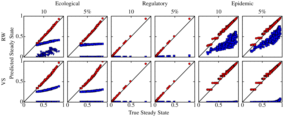
Figure 4: Predicted steady states when vertex degrees $\delta_{i}$ are available. The diagonal line is perfect prediction. Our method (red) is nearly perfect, while the naive method (blue) is a disaster. Often, the steady states just converge to 0 for the naive method.

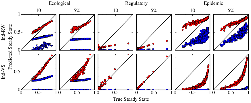
Figure 5: Predicted steady-states when only the induced subgraph is available and vertex degrees must be estimated. Our method (red) significantly outperforms naive, but performance drops compared to Figure 4, because estimating vertex degrees from observed induced degrees is tough.

For Ind-RW, the network average degree $\langle\delta\rangle$ is needed to estimate true degrees (in addition to $n$). There are methods to estimate $\langle\delta\rangle$ (?; ?; ?; ?), but they use more powerful queries than the induced subgraph from a simple random walk can provide. The complication with the simple random walk is that it is a degree-biased sampling of vertices. This bias can be corrected with a Metropolis-Hastings random walk (?), but that requires knowledge of vertex degrees.

One can analyze the bias and variance of our estimators using the importance sampling framework that samples vertices according to the proposal distribution $q$ (?; ?; ?) (uniform or degree-biased). We postpone the details to the full paper.

5 Results

We tested our approach on the three popular dynamical systems in Table 1 and two corresponding networks for each dynamical system (see Table 2).

Each dynamical system contains several parameters which are set as in (?) for ecology and gene regulation, and as in (?) for epidemics. We compare the performance of different subgraph-sampling (RW, VS, Ind-RW, Ind-VS), with sample size $m=10$ (constant size) and $m=0.05n$ (constant fraction). We average results over several subgraphs. When a vertex is sampled in multiple subgraphs, we report the average predicted steady-state.

Given a subgraph, we solve (6) to estimate the true steady-states of vertices in the subgraph, for which we need $\delta_{i}$ (true degree) and $x_{\text{eff}}$ (effective external state). To get $x_{\text{eff}}$, we need $\beta$ to solve (14). For $\delta_{i}$ and $\beta$, we use the estimates in Section 4.1. In solving  (14), there can be one stable attractor or more than one stable attractors (there can also be unstable attractors). When there are more than one stable attractor, the system can equilibrate at multiple steady-states.

First, we consider sampling methods that obtain vertex degrees $\delta_{i}$ (RW, VS), where only $\beta$ needs to be estimated. The results in Figure 4 show that our approach (red) is remarkable at revealing the true steady-state, even from tiny subgraphs. We get near perfect results from just 10 vertices of a multi-thousand vertex graph. This is all the more impressive given that the current state-of-the-art, i.e., the naive approach (blue), is more or less a disaster. We emphasize that the naive method is the only method currently used by researchers in the field, and it simply fails. In the ecological application, the naive method even identifies multiple steady-states, one of which sends all species to extinction.

When only induced subgraphs are available (Ind-RW, Ind-VS), see Figure 5, our methods are still much better than naive, but the performance drops. Estimating individual degrees from induced degrees is hard. Parameters like the resilience $\beta$ are global and can be extracted accurately from subgraphs. Local parameters like vertex degree get severely distorted. More details on how degree and resilience estimations are affected by induced subgraph sampling is deferred. For vertex sampling, our estimator is unbiased, but for random walks, our estimators are based on the approximation of independent degree-biased sampling. This approximation can break down.

Open Question. How should one estimate vertex degrees from induced subgraphs of random walks? How does the estimator depend on the network properties?

We also observe from Figure 5 that for induced subgraphs, the performance of our approach (and the naive method) depends strongly on the subgraph sampling methods, depending on the network structure and the nonlinear dynamics.

Open Question. What are the factors which influence the choice of subgraph sampling method? For example when is RW better than VS?

6 Discussion

We addressed a prevalent problem. Consider this scenario. A biologist has the favorite part of an ecosystem, their favorite 10-species, and carefully collects their relationships which are summarized in the adjacency matrix $A^{(s)}$. The biologist even knows how species interact, the dynamical system (1). The biologist carefully simulates the system to steady-state and finds that all species are going extinct. This is scary, but the result is just plain wrong. You cannot restrict a coupled nonlinear system to your favorite part of the network and expect even close to correct conclusions by just analyzing that part in isolation. One solution is to collect the full network and analyze the full system. There are two problems. First, we can’t collect the full network. Second, simulating the full system to equilibrium is prohibitive in terms of convergence time. So the only feasible solution for learning the true steady states of the observed incomplete network is to somehow account for the external impact on the local system. This was our approach. In a mean field approximation, the external impact reduces to a single parameter $x_{\text{eff}}$ which depends only on the network’s resilience $\beta$, a topological parameter. We showed how to estimate resilience, depending on how the subgraph is sampled. Our results on real networks with corresponding dynamics gave spectacular success – we accurately recover steady-states from just 10-vertex subgraphs of thousand-vertex networks.

There are several interesting future questions. The natural one is to find improved estimates of resilience that extend to other sampling methods (snowball sampling, edge sampling etc). A critical direction, which we address in forthcoming work, is the inverse problem. Suppose the steady-states are known. For example, the abundance of your 10 favorite monkey species is known. Can one infer the correct dynamical system $f(\cdot),g(\cdot,\cdot)$? Currently, the dynamics are fit to the observed steady-states for the partial network (?; ?; ?; ?; ?). This is wrong and will produce the incorrect dynamics. It is no surprise, therefore, that the inferred dynamics keeps changing as more data is collected (?; ?; ?; ?). It is absolutely critical to account for the external impact in the inference process.

7 Acknowledgements

This work was partially supported by the ONR Contract N00014-15-1-2640.

References

- [Ahmed, Neville, and Kompella 2011] Ahmed, N.; Neville, J.; and Kompella, R. R. 2011. Network sampling via edge-based node selection with graph induction. Computer Science Technical Reports.
- [Allee et al. 1949] Allee, W. C.; Park, O.; Emerson, A. E.; Park, T.; Schmidt, K. P.; et al. 1949. Principles of animal ecology. Technical report, Saunders Company Philadelphia, Pennsylvania, USA.
- [Alon 2006] Alon, U. 2006. An introduction to systems biology: design principles of biological circuits. Chapman and Hall/CRC.
- [Arroyo, Armesto, and Primack 1985] Arroyo, M. T. K.; Armesto, J. J.; and Primack, R. B. 1985. Community studies in pollination ecology in the high temperate andes of central chile ii. effect of temperature on visitation rates and pollination possibilities. Plant Systematics and Evolution 149(3-4):187–203.
- [Barzel and Barabási 2013] Barzel, B., and Barabási, A.-L. 2013. Universality in network dynamics. Nature Physics 9(10):673.
- [Bongard and Lipson 2007] Bongard, J., and Lipson, H. 2007. Automated reverse engineering of nonlinear dynamical systems. PNAS 104(24):9943–9948.
- [Brunton, Proctor, and Kutz 2016] Brunton, S. L.; Proctor, J. L.; and Kutz, J. N. 2016. Discovering governing equations from data by sparse identification of nonlinear dynamical systems. PNAS 113(15):3932–3937.
- [Clements and Long 1923] Clements, F. E., and Long, F. L. 1923. Experimental pollination: an outline of the ecology of flowers and insects. Number 336. Carnegie Institution of Washington.
- [Cochran 1977] Cochran, W. G. 1977. Sampling technique.
- [Dasgupta, Kumar, and Sarlos 2014] Dasgupta, A.; Kumar, R.; and Sarlos, T. 2014. On estimating the average degree. In Proc. Conf. WWW, 795–806.
- [Dodds and Watts 2005] Dodds, P. S., and Watts, D. J. 2005. A generalized model of social and biological contagion. Journal of Theoretical Biology 232(4):587–604.
- [Edwards and Anderson 1975] Edwards, S. F., and Anderson, P. W. 1975. Theory of spin glasses. Journal of Physics F: Metal Physics 5(5):965.
- [Gao, Barzel, and Barabási 2016] Gao, J.; Barzel, B.; and Barabási, A.-L. 2016. Universal resilience patterns in complex networks. Nature 530(7590):307.
- [Gao et al. 2014] Gao, J.; Liu, Y.-Y.; D’souza, R. M.; and Barabási, A.-L. 2014. Target control of complex networks. Nature Communications 5:5415.
- [Ghahramani and Roweis 1999] Ghahramani, Z., and Roweis, S. T. 1999. Learning nonlinear dynamical systems using an em algorithm. In Advances in NIPS, 431–437.
- [Gjoka, Kurant, and Markopoulou 2013] Gjoka, M.; Kurant, M.; and Markopoulou, A. 2013. 2.5 k-graphs: from sampling to generation. In INFOCOM’13, 1968–1976. IEEE.
- [Guimera et al. 2003] Guimera, R.; Danon, L.; Diaz-Guilera, A.; Giralt, F.; and Arenas, A. 2003. Self-similar community structure in a network of human interactions. Phys. Rev. E 68(6):065103.
- [Hübler et al. 2008] Hübler, C.; Kriegel, H.-P.; Borgwardt, K.; and Ghahramani, Z. 2008. Metropolis algorithms for representative subgraph sampling. In ICDM’08, 283–292. IEEE.
- [Hufnagel, Brockmann, and Geisel 2004] Hufnagel, L.; Brockmann, D.; and Geisel, T. 2004. Forecast and control of epidemics in a globalized world. PNAS 101(42):15124–15129.
- [Hui 2006] Hui, C. 2006. Carrying capacity, population equilibrium, and environment’s maximal load. Ecological Modelling 192(1-2):317–320.
- [Ionides, Bretó, and King 2006] Ionides, E. L.; Bretó, C.; and King, A. A. 2006. Inference for nonlinear dynamical systems. PNAS 103(49):18438–18443.
- [Karlebach and Shamir 2008] Karlebach, G., and Shamir, R. 2008. Modelling and analysis of gene regulatory networks. Nature Reviews Molecular Cell Biology 9(10):770.
- [Katzir, Liberty, and Somekh 2011] Katzir, L.; Liberty, E.; and Somekh, O. 2011. Estimating sizes of social networks via biased sampling. In Proc. Conf. WWW, 597–606. ACM.
- [Klusowski and Wu 2018] Klusowski, J. M., and Wu, Y. 2018. Counting motifs with graph sampling. In Bubeck, S.; Perchet, V.; and Rigollet, P., eds., Proceedings of the 31st Conference On Learning Theory, volume 75 of Proceedings of Machine Learning Research, 1966–2011. PMLR.
- [Kunegis 2013] Kunegis, J. 2013. KONECT: The Koblenz Network Collection. In Proc. Conf. WWW, 1343–1350. ACM.
- [Kurant, Butts, and Markopoulou 2012] Kurant, M.; Butts, C. T.; and Markopoulou, A. 2012. Graph size estimation. arXiv preprint arXiv:1210.0460.
- [Kurant, Markopoulou, and Thiran 2011] Kurant, M.; Markopoulou, A.; and Thiran, P. 2011. Towards unbiased BFS sampling. IEEE Journal on Selected Areas in Communications 29(9):1799–1809.
- [Lee et al. 2002] Lee, T. I.; Rinaldi, N. J.; Robert, F.; Odom, D. T.; Bar-Joseph, Z.; Gerber, G. K.; Hannett, N. M.; Harbison, C. T.; Thompson, C. M.; Simon, I.; et al. 2002. Transcriptional regulatory networks in Saccharomyces cerevisiae. Science 298(5594):799–804.
- [Leskovec and Faloutsos 2006] Leskovec, J., and Faloutsos, C. 2006. Sampling from large graphs. In Proc. Conf. ACM SIGKDD, 631–636. ACM.
- [Lotka 1910] Lotka, A. J. 1910. Contribution to the theory of periodic reactions. The Journal of Physical Chemistry 14(3):271–274.
- [Pastor-Satorras and Vespignani 2001] Pastor-Satorras, R., and Vespignani, A. 2001. Epidemic spreading in scale-free networks. Phys. Rev. Lett. 86(14):3200.
- [Ribeiro and Towsley 2010] Ribeiro, B., and Towsley, D. 2010. Estimating and sampling graphs with multidimensional random walks. In Proc. Conf. Internet Measurement, 390–403.
- [Rossi and Ahmed 2015] Rossi, R., and Ahmed, N. 2015. The network data repository with interactive graph analytics and visualization. In AAAI.
- [Schmidt and Lipson 2009] Schmidt, M., and Lipson, H. 2009. Distilling free-form natural laws from experimental data. Science 324(5923):81–85.
- [Seshadhri, Pinar, and Kolda 2014] Seshadhri, C.; Pinar, A.; and Kolda, T. G. 2014. Wedge sampling for computing clustering coefficients and triangle counts on large graphs. Statistical Analysis and Data Mining: The ASA Data Science Journal 7(4):294–307.
- [Stumpf and Wiuf 2005] Stumpf, M. P., and Wiuf, C. 2005. Sampling properties of random graphs: the degree distribution. Phys. Rev. E 72(3):036118.
- [Theodoridis 2015] Theodoridis, S. 2015. Machine learning: a Bayesian and optimization perspective. Academic Press.
- [Wu 1982] Wu, C.-F. 1982. Estimation of variance of the ratio estimator. Biometrika 69(1):183–189.
- [Zhang, Kolaczyk, and Spencer 2015] Zhang, Y.; Kolaczyk, E. D.; and Spencer, B. D. 2015. Estimating network degree distributions under sampling: An inverse problem, with applications to monitoring social media networks. Annals of Applied Statistics 9:166–199.