FASiM: A Framework for Automatic Formal Analysis of Simulink Models of Linear Analog Circuits

Abstract

Simulink is a graphical environment that is widely adapted for the modeling and the Laplace transform based analysis of linear analog circuits used in signal processing architectures. However, due to the involvement of the numerical algorithms of MATLAB in the analysis process, the analysis results cannot be termed as complete and accurate. Higher-order-logic theorem proving is a formal verification method that has been recently proposed to overcome these limitations for the modeling and the Laplace transform based analysis of linear analog circuits. However, the formal modeling of a system is not a straightforward task due to the lack of formal methods background for engineers working in the industry. Moreover, due to the undecidable nature of higher-order logic, the analysis generally requires a significant amount of user guidance in the manual proof process. In order to facilitate industrial engineers to formally analyze the linear analog circuits based on the Laplace transform, we propose a framework, FASiM, which allows automatically conducting the formal analysis of the Simulink models of linear analog circuits using the HOL Light theorem prover. For illustration, we use FASiM to formally analyze Simulink models of some commonly used linear analog filters, such as Sallen-key filters.

I Introduction

In the past couple of decades, the analog and mixed signal and integrated circuit design has experienced dramatic changes due to their wider utility in the embedded systems, such as mobile phones, cameras and other electronic appliances based on the growing demands of the consumer marketplace. These changes involve reduction in their sizes, operating voltages and power consumption capabilities, which resulted in to an enormous increase in complexities of these circuits due to the placement of a large amount of analog and digital components on a small area. Due to this rapidly growing market of the embedded systems and complexities of their corresponding design, the accuracy of the design and the associated analysis has become a dire need, since a small design flaw can result into undesirable consequences, like heavy financial losses that can directly effect the company developing these designs and the market as well.

Linear analog circuits are a vital part of the integrated circuits and their accurate design and analysis is of utmost importance. For example, they are a fundamental component of a Complementary Metal–oxide–semiconductor (CMOS) image sensor based digital camera, which provides significant advantages in comparison to the traditional Charge-coupled Device (CCD) imaging systems [1, 2]. Figure 1 presents a typical image sensor based signal processing architecture that is used for imaging and mixed-signal processing. It involves an analog signal acquisition from the image sensor. To improve the quality of the image by reducing the random image noise, some analog preprocessing algorithms, composed of linear analog circuits (spatial filters), are applied. The resultant analog signal is converted to a digital signal using an A/D converter, which is then used for further digital image processing [1, 2]. Being a major part of a image processing architecture, there is a dire need of accurate design and analysis of linear analog circuits.

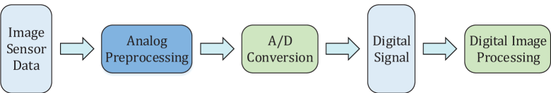
Figure 1: Image Sensor based Signal Processing Architecture

One of the most challenging aspects of modeling and analyzing linear analog circuits is to capture their continuous dynamics in their corresponding mathematical models, which are based on physical laws. For example, in order to model the voltages and currents passing through the electrical components and their interaction, we have to use circuit’s governing laws, such as Kirchhoff’s Voltage Law (KVL) and Kirchhoff’s Current Law (KCL). These mathematical models are further used to derive the corresponding linear differential equations of the underlying system. The next step is to solve these equations to study properties of the system, such as transfer function and frequency response. However, solving these equations in time domain is not quite straightforward due to the involvement of the differential and integral operators. The Laplace transform [3], an integral based transform method, is often used to solve these equations by converting the time domain models (differential equations) to their corresponding algebraic equations in the frequency domain, i.e., the $s$-domain, which allows us to transform the integral and differential operators to their corresponding division and multiplication operators. These equations can now be solved in a quite straightforward way to obtain the corresponding transfer function [3] and frequency response [3] of the system or solution of the differential equations in frequency domain. Finally, the uniqueness of the Laplace transform is utilized to obtain the solution of these differential equations in time domain. All these properties play a crucial role in designing a reliable analog circuit.

Simulink [4] is a graphical environment that provides the modeling of a system in the forms of blocks and supports its corresponding analysis using MATLAB. It has been widely used for modeling of analog circuits and performing their transfer function based analysis [5]. To perform the Laplace transform based analysis of a linear analog circuit, we generally develop its Simulink model, which is further analyzed to study its various characteristics, such as transfer function and frequency response. Moreover, the theory of the Laplace transform, available in MATLAB, can be used for analyzing the continuous dynamics of the circuits. For example, the MATLAB function laplace (f) accepts a time domain function f or any linear differential equation and provides its corresponding algebraic expression, which can further simplified to obtain the corresponding transfer function, i.e., the system’s input-output relationship in the $s$-domain. This transformation of the time domain model to its corresponding algebraic expressions in $s$-domain can also be obtained using some other variants of laplace, i.e., laplace (f,transVar) and laplace (f,var,transVar) that provide the flexibility for the selection of the time domain variable and corresponding frequency domain variable other than $t$ and $s$, respectively. Similarly, the function ilaplace (F) takes a $s$-domain function F and returns the corresponding time domain model, i.e., the differential equation or its associated solution in the time domain. The other variants that are also used for the transformation of the algebraic expressions in $s$-domain to their corresponding time domain representations are ilaplace (F,transVar) and ilaplace (F,var,transVar). However, these functions are based on various numerical algorithms that usually involve approximations of the mathematical expressions or results and thus cannot be relied on when performing the analysis of the linear analog circuits used in the safety and mission-critical domains, like transportation, healthcare and energy distribution.

Higher-order-logic theorem proving [6], i.e., a widely used formal verification method, has been used to overcome the inaccuracy limitations of the above-mentioned analysis of the linear analog circuits. It is a computer based mathematical analysis technique that requires developing a mathematical model of the given system in higher-order logic and the formal verification of its intended behaviour, as a mathematically specified property, based on mathematical reasoning within the sound core of a theorem prover. Based on the same motivation, the Laplace transform has been recently formalized in the HOL Light theorem prover and it has been utilized to perform the transfer function analysis of the Linear Transfer Converter (LTC) circuit [7], Sallen-key low-pass filters [8] and a $4$-$\pi$ soft error crosstalk model [9]. However, utilizing the Laplace transform theory of HOL Light for formally analyzing any system is not a straightforward task as it requires developing a mathematical model and user guidance in the proof process. In this paper, to facilitate engineers for formally analyzing the linear analog circuits, we propose a framework, FASiM, which provides the automatic formal analysis of the Simulink models of these circuits using the formalized Laplace transform theory developed in HOL Light. The idea is to extract the transfer function of the underlying system after simulating its model developed in Simulink. This extracted transfer function is automatically translated, using a translator developed as a part of this framework, to its corresponding transfer function in HOL Light, which is then used for the automatic formal analysis of the linear analog circuit using the Laplace transform. Based on our proposed framework, the user only needs to develop the Simulink model of the circuit and the rest of the formal analysis is done almost automatically. For illustration, we use our proposed framework for the automatic formal analysis of the Simulink models of some commonly used analog circuits like Sallen-key filters, etc.

II Related Work

To overcome the inherent limitations of the computer-simulation based analysis, formal methods have been previously used for analyzing the Simulink models as well. The MathWorks introduced a verification tool, Simulink Design Verifier (SLDV) [10], which is a component of the Simulink environment and is used for formally verifying the Simulink models. SLDV is primarily based on the widely used automated formal verification techniques, i.e., automated theorem proving and model-checking, for the formal verification of the Simulink model of a system and in the case of a failure, it generates a counter-example, which can be used to detect the bug/error in the underlying system’s model. Similarly, Silva et al. [11] provided a computational tool, CheckMate, which is used for formally verifying the hybrid systems. It involves modeling the underlying system using hybrid automata and verification of its associated properties, specified as ACTL formulae, using model checking. Reicherdt et al. [12] proposed to conduct the formal verification of the discrete-time MATLAB/Simulink models using Microsoft Boogie program verifier. It involves the automatic translation of MATLAB/Simulink models into the Boogie verification language, which allows developing first-order logic based models of the system and their verification using the automated theorem prover Z3. Similarly, Bostrom [13] proposed an approach for the contract-based verification of the Simulink models. It involves translating the Simulink models, viewed as Synchronous Data Flow (SDF) graphs, to their corresponding functionally equivalent sequential program statements, which are further analyzed using the automated theorem prover Z3. Joshi et al. [14] proposed an approach for the verification of the discrete time MATLAB/Simulink models using the SCADE design verifier. It includes the translation of the MATLAB/Simulink models to the synchronous data flow language, Lustre, which are further used for the model-based safety analysis using SCADE. However, due to the inherent computational limitations of the associated formal methods, i.e., less-expressiveness and abstraction in automated theorem proving, and discretization of the continuous models and state-space explosion in model checking, the above-mentioned approaches cannot be termed as accurate and complete when analyzing the complex systems exhibiting continuous dynamics.

Higher-order-logic theorem proving has also been used for formally analyzing the Simulink models. Chen et al. [15] utilized the Prototype Verification System (PVS) theorem prover for the formal verification of Simulink models. Their proposed approach is based on transforming the Simulink models to their corresponding Timed Interval Calculus (TIC) models, which are further analyzed using PVS. However, this approach cannot be utilized for the Laplace transform based analysis of the systems exhibiting the continuous dynamics, which is the main scope of the paper.

III Proposed Framework

Our proposed framework, FASiM, for the automatic formal analysis of the Simulink models of the linear analog circuits using the Laplace transform theory of the HOL Light theorem prover is depicted in Figure 2. The first step is to develop the Simulink model of a linear analog circuit. Next, we need to simulate/analyze the Simulink model to obtain its corresponding transfer function, which represents the input-output relationship in the $s$-domain and is mathematically expressed for the series RLC circuit as:

$$\dfrac{V_{o}(s)}{V_{i}(s)}=\dfrac{1}{s^{2}LC+sRC+1}$$

Now, in order to perform the formal analysis of a Simulink model, we need to transform this transfer function to its corresponding transfer function in HOL Light. For this purpose, our framework first extracts the coefficients of the numerator and denominator of the transfer function as lists in XML. Next, a translator is involved that automatically translates these XML lists of coefficients to their corresponding lists in HOL Light (ML). The HOL Light lists are further used to formalize the corresponding transfer function and perform the automatic analysis of the linear analog circuits using the Laplace transform theory of HOL Light theorem prover, i.e., to formally verify the transfer function and solution of the corresponding time domain models capturing the dynamics of the circuits. Our proposed framework, FASiM, has twofold advantages: 1) It provides a rigourous analysis of Simulink models of the linear analog circuits unlike their traditional analysis, which is based on the unverified numerical algorithms of MATLAB and thus cannot be trusted for safety-critical applications 2) The translator, developed as a part of this framework, enables the engineers to use the library of the Laplace transform in HOL Light for the automatic formal analysis without learning the tool and its associated language, which was not possible in the earlier analysis [7, 8, 9, 16, 17, 18].

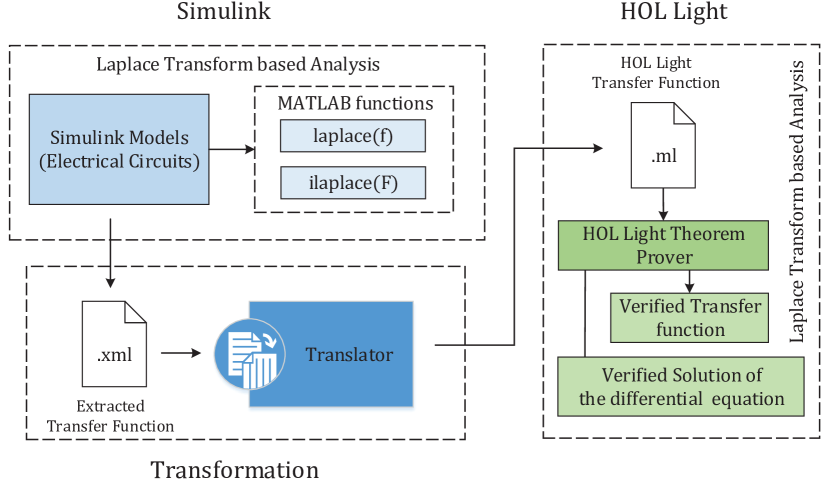
Figure 2: Proposed Framework

IV Preliminaries

TABLE I: Laplace Transform

Mathematical Form	Formalized Form
Laplace Transform
$\begin{array}[]{lcl}\mathcal{L}[f(t)]=F(s)=\\ \hskip 28.45274pt\int_{0}^{\infty}{f(t)e^{-st}}dt,\ s\ \epsilon\ \mathds{C}\end{array}$	$\begin{array}[]{lcl}\textup{{ $\vdash_{\mathtt{def}}$ $\forall$s f. {\color[rgb]{0,0,1}{l}aplace\_transform} f s = }}\\ \textup{{ integral \{t $|$ \&0 $\leq$ drop t\} ($\lambda$t. cexp ($--$(s $\ast$ Cx (drop t))) $\ast$ f t) }}\end{array}$
Laplace Existence
$f$ is piecewise smooth and is of exponential order on the positive real line	$\begin{array}[]{lcl}\textup{{ $\vdash_{\mathtt{def}}$ $\forall$s f. {\color[rgb]{0,0,1}{l}aplace\_exists} f s $\Leftrightarrow$ }}\\ \textup{{ ($\forall$b. f piecewise\_differentiable\_on interval [lift (\&0),lift b]) $\wedge$ }}\\ \textup{{ ($\exists$M a. Re s $>$ drop a $\wedge$ exp\_order\_cond f M a) }}\end{array}$
Exponential-order Condition
There exist a constant $a$ and a positive constant $M$ such that $|f(t)|\leq Me^{at}$	$\begin{array}[]{lcl}\textup{{ $\vdash_{\mathtt{def}}$ $\forall$f M a. {\color[rgb]{0,0,1}{e}xp\_order\_cond} f M a $\Leftrightarrow$ }}\\ \textup{{ \&0 $<$ M $\wedge$ ($\forall$t. \&0 $\leq$ t $\Rightarrow$ norm (f (lift t)) $\leq$ M $\ast$ exp (drop a $\ast$ t)) }}\end{array}$
Differential Equation of Order $n$
$\begin{array}[]{lcl}\textit{Differential}\ \textit{Equation}=\sum\limits_{k=0}^{n}{{\alpha}_{k}\dfrac{d^{k}f}{{dt}^{k}}}\end{array}$	$\begin{array}[]{lcl}\textup{{ $\vdash_{\mathtt{def}}$ $\forall$n f t. {\color[rgb]{0,0,1}{d}iff\_eq\_n\_order} n lst f t = }}\\ \textup{{ vsum (0..n) ($\lambda$k. EL k lst $\ast$ higher\_order\_derivative k f t) }}\end{array}$
Uniqueness of the Laplace Transform
If the Laplace transforms of two functions $f$ and $g$ are equal, i.e., $\mathcal{L}[f(t)]=\mathcal{L}[g(t)]$, then both functions $f$ and $g$ are the same, i.e., $f(t)=g(t)$ for all $0\leq t$	$\begin{array}[]{lcl}\textup{{ $\vdash_{\mathtt{thm}}$ $\forall$f g r. {[A1]} \&0 $<$ Re r $\wedge$ }}\\ \textup{{ {[A2]} ($\forall$s. Re r $\leq$ Re s $\Rightarrow$ laplace\_exists f s) $\wedge$ }}\\ \textup{{ {[A3]} ($\forall$s. Re r $\leq$ Re s $\Rightarrow$ laplace\_exists g s) $\wedge$ }}\\ \textup{{ {[A4]} ($\forall$s. Re r $\leq$ Re s $\Rightarrow$ laplace\_transform f s = laplace\_transform g s) }}\\ \textup{{ \hskip 28.45274pt $\Rightarrow$ ($\forall$t. \&0 $\leq$ drop t $\Rightarrow$ f t = g t) }}\end{array}$

This section presents a brief introduction to higher-order-logic theorem proving, the HOL Light theorem prover and its Laplace transform theory, which is extensively used in the rest of the paper.

IV-A Higher-order-logic Theorem Proving

Theorem proving [6] involves constructing the mathematical proofs using a computer program based on axioms and hypothesis. Theorem provers have been extensively used for formalizing classical mathematics, e.g., the formal proof of Kepler conjecture [19], the formal library of Euclidean space in HOL Light theorem prover [20] and for verifying many hardware [21] and software [22] systems. The main idea is to verify a system by formally proving its various properties in the form of mathematical theorems expressed in some appropriate logic, which can be propositional, first-order or higher-order logic.

Based on the decidability or undecidability of the underlying logic, theorem proving can be automatic or interactive. For example, a computer program can automatically verify the theorems about sentences expressed in the propositional logic due to the decidability of this logic whereas the higher-order logic is undecidable and thus verifying proof goals expressed in this logic requires explicit user guidance in an interactive manner.

IV-B HOL Light Theorem Prover

HOL Light [23] is a higher-order-logic theorem prover that ensures secure theorem proving using the Objective CAML (OCaml) language, which is a variant of the strongly-typed functional programming language ML. HOL Light has the smallest trusted core (i.e., approximately $400$ lines of OCaml code) compared to all other HOL theorem provers and the underlying logic kernel has been verified in the CakeML project [24]. HOL Light users can interactively verify theorems by applying the available proof tactics and proof procedures. A HOL Light theory consist of types, constants, definitions and theorems. HOL Light theories are built in a hierarchical fashion and new theories can inherit the definitions and theorems of their parent theories. HOL Light consists of a rich set of formalized theories of multivariable calculus and the Laplace transform theories, which are extensively used in the proposed work.. Table I presents some definitions from the Laplace transform theory of HOL Light, which includes the Laplace transform, Laplace existence and the exponential-order conditions, the differential equation of order $n$ and the uniqueness of the Laplace transform. Interested readers can refer to [7] for more details about this theory.

V XML to HOL Light (ML) Translator

The main components of our XML to HOL Light (ML) translator are depicted in Figure 3. It consists of four blocks, namely parser, Intermediate Representation (IR) generator, code optimizer and code generator. Our translator accepts an XML file containing the lists of coefficients of the numerator and denominator of the corresponding transfer function of the underlying system. The first block of the translator, i.e., parser, scans the tags and sub-tags of the XML file to extract the tags and the contents of the numerator and denominator of the transfer function.

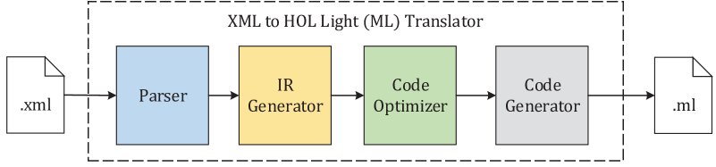
Figure 3: XML to HOL Light (ML) Translator

The information extracted from the XML file by parser is then provided to the second block, i.e., IR generator, which generates the intermediate representation of the acquired data. This representation involves restructuring of the data in such a way that it facilitates the execution of the subsequent steps towards generating the ML representation while retaining the contents of the tags related data.

Next, the intermediate representation produced by the IR generator is passed to the third block, i.e., code optimizer, which optimizes the coefficients of the numerator and denominator. The coefficients extracted by the IR generator have the same syntax as they are represented in MATLAB, i.e., scientific (exponential) notation ($E^{n}$) for the large values of the exponent $n$ (in both command window and workspace) and thus it requires a conversion from the scientific notation to standard form. Moreover, in HOL Light (ML), the decimal numbers and the integer literals of data-type $\mathds{R}$ are represented in two different forms. Thus, in order to make both these representations (XML and HOL Light representations) coherent, the code optimizer performs these conversions to remodel the IR according to the language of HOL Light.

Finally, the optimized code is used by the fourth block, i.e., code generator, to generate the output ML file, which can be directly used by HOL Light.

It is to be noted that the purpose of translator is to aid the process of automatic conversion of the Simulink models and it is, itself, not formally verified so it may lead to erroneous translated lists of the coefficients and the associated formal models of the transfer function just like the case with the manual formalization process. However, as the translated model undergoes the formal verification phase using HOL Light, so there is a high probability of detecting these kinds of flaws during this verification.

VI Application: Linear Analog Filters

Analog filters are used for the purpose of signal filtering and thus allow the passage of signals over a certain range of frequencies. They are of various types, i.e., low-pass, high-pass, band-pass and band-stop etc, based on the range of the frequencies of the input signals that are allowed to pass. For example, a low-pass filter only allows the passage of the signals having frequencies lower than the cut-off frequency and thus reduces the random image noise for a CMOS sensor based camera. To illustrate the practical utilization of our proposed framework, FASiM, we develop a library, which provides the automatic analysis of the Simulink models of various filters, i.e., RC low-pass, first-order all-pass, second-order all-pass, Sallen-key low-pass, Sallen-key high-pass, multiple feedback low-pass, multiple feedback high-pass, multiple feedback band-pass, Boctor notch low-pass and Boctor notch high-pass filters. However, due to the space limitation, we only present the formal analysis of the Simulink model of the Sallen-key low-pass filter.

Sallen-key filters are the linear analog filters, which are extensively used in various applications, such as analog preprocessors, analog-to-digital converters, audio crossover and radio transmitters. The Simulink model for the Sallen-key low-pass filter is depicted in Figure 4. The components $R_{1}$, $R_{2}$, $R_{3}$ and $R_{4}$ represent the resistors, whereas, $C_{1}$ and $C_{2}$ models the corresponding capacitors of the filter. Similarly, $R_{L}$ represents the load at the output of the filter. The differential equation modeling the dynamics of the filter for the input voltage $v_{i}$ and the output voltage $v_{o}$ is represented as:

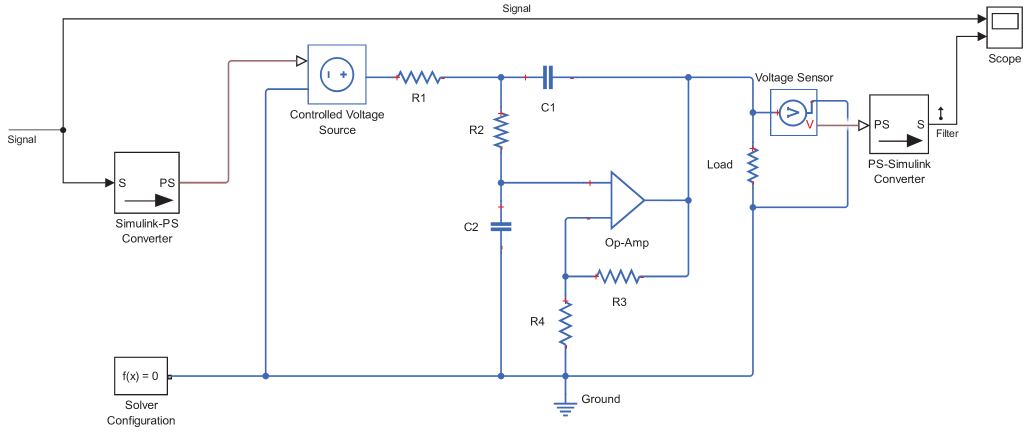
Figure 4: Sallen-key Low-pass Filter

$$\begin{split}R_{1}R_{2}R_{4}C_{1}C_{4}\dfrac{d^{2}v_{o}}{dt^{2}}+(R_{1}R_{4}C_{2}+R_{2}R_{4}C_{2}-R_{1}R_{3}R_{4}C_{1})\\ \dfrac{dv_{o}}{dt}+R_{4}v_{o}=(R_{3}+R_{4})v_{i}\end{split}$$ (1)

Next, we simulate the Simulink model of the filter using the values of its various components as $R_{1}$ = $R_{2}$ = $16K\Omega$, $R_{3}$ = $R_{4}$ = $30K\Omega$, $C_{1}$ = $C_{2}$ = $1nF$, $R_{L}$ = $10K\Omega$. The corresponding transfer function obtained by the simulation of the filter model is mathematically expressed as:

$$\dfrac{V_{o}(s)}{V_{i}(s)}=\dfrac{7.813\times{10}^{9}}{s^{2}+6.25\times{10}^{4}s+3.906\times{10}^{9}}$$ (2)

where the coefficients of the numerator and denominator of the transfer function in the above equation are the rounded off values of the coefficients that are obtained from simulations. However, using our proposed framework, we extract their exact values (from MATLAB’s workspace), i.e., before applying the round-off process, in lists in XML, i.e., numerator = $[7812500000.48828]$ and denominator = $[1\ 62500.0000039063\ 3906249999.75586]$. These XML lists of coefficients are further converted automatically to HOL Light lists using our XML to HOL Light (ML) translator. Next, these HOL Light lists are used to model the corresponding transfer function of the filter. Finally, in order to verify the transfer function, we first model the corresponding differential equation of the filter in HOL Light as:

Definition 1.

$\vdash_{\mathtt{def}}$ inlst_SKLP_filter =
                                 $\left[\texttt{Cx}\left(\texttt{\#7812500000.48828}\right)\right]$
  $\vdash_{\mathtt{def}}$ outlst_SKLP_filter =
    $\left[\texttt{Cx}\left(\texttt{\#3906249999.75586}\right);\texttt{Cx}\left(\texttt{\#62500.0000039063}\right);\texttt{Cx}\left(\&1\right)\right]$
  $\vdash_{\mathtt{def}}$ diff_eq_SKLP_filter VI V0 $\Leftrightarrow$
   ($\forall$t. diff_eq_n_order 2 outlst_SKLP_filter V0 t =
          diff_eq_n_order 0 inlst_SKLP_filter VI t)

where the HOL Light function diff_eq_n_order models the linear differential equation of order $n$, given in Table I. The symbol # is used to represent a decimal number of data-type $\mathds{R}$ in HOL Light.

Now, we formally verify the corresponding transfer function as the following HOL Light theorem:

Theorem 1.

$\vdash_{\mathtt{thm}}$ $\forall$VI V0 s.
   [A1] ($\forall$t. differentiable_higher_deriv 0 VI t) $\wedge$
   [A2] ($\forall$t. differentiable_higher_deriv 2 V0 t) $\wedge$
   [A3] zero_init_conditions 1 V0 $\wedge$
   [A4] laplace_transform VI s $\neq$ Cx (&0) $\wedge$
   [A5] ($\texttt{s}^{\texttt{2}}$ + Cx $\left(\texttt{\#62500.0000039063}\right)$ $\ast$ s +
                       Cx $\left(\texttt{\#3906249999.75586}\right)$ $\neq$ Cx (&0)) $\wedge$
   [A6] laplace_exists_higher_deriv 0 VI s $\wedge$
   [A7] laplace_exists_higher_deriv 2 V0 s $\wedge$
   [A8] ($\forall$t. diff_eq_SKLP_filter VI V0 t) $\wedge$
             
              $\Rightarrow$ $\dfrac{\texttt{laplace\_transform V0 s}}{\texttt{laplace\_transform VI s}}$ =
             
   $\dfrac{\texttt{Cx}\left(\texttt{\#7812500000.48828}\right)}{\texttt{s}^{\texttt{2}}\texttt{+ Cx}\left(\texttt{\#62500.0000039063}\right)\ast\texttt{s + Cx}\left(\texttt{\#3906249999.75586}\right)}$

The assumptions A1-A2 provide the differentiability conditions for the input VI and output V0 up to the order $0$ and $2$, respectively. The assumption A3 presents the zero initial conditions for the function V0. The assumptions A4-A5 express the design constraints for the Sallen-key low-pass filter. Similarly, the assumptions A6-A7 ensure that the Laplace transform of the functions VI and V0 exist up to order $0$ and $2$, respectively. The assumption A8 provides the differential equation model of the underlying filter. Finally, the conclusion represents the corresponding transfer function (Equation (2)). The verification of Theorem 1 is done automatically using the automatic tactic DIFF_EQ_2_TRANS_FUN_TAC, which is developed as a part of our theory of the Laplace transform in HOL Light. It requires the differential equation and the transfer function of the underlying system and automatically verifies the theorem corresponding to the transfer function of the system.

Next, we formally verify the differential equation of the Sallen-key low-pass filter based on its transfer function as:

Theorem 2.

$\vdash_{\mathtt{thm}}$ $\forall$VI V0 r.
   [A1] ($\forall$t. differentiable_higher_deriv 0 VI t) $\wedge$
   [A2] ($\forall$t. differentiable_higher_deriv 2 V0 t) $\wedge$
   [A3] zero_init_conditions 1 V0 $\wedge$
   [A4] ($\forall$s. Re r $\leq$ Re s $\Rightarrow$ ($\texttt{s}^{\texttt{2}}$ + Cx $\left(\texttt{\#62500.0000039063}\right)$
              $\ast$ s + Cx $\left(\texttt{\#3906249999.75586}\right)$ $\neq$ Cx (&0))) $\wedge$
   [A5] ($\forall$s. Re r $\leq$ Re s $\Rightarrow$
                       laplace_transform VI s $\neq$ Cx (&0)) $\wedge$
   [A6] &0 $<$ Re r $\wedge$
   [A7] ($\forall$s. Re r $\leq$ Re s $\Rightarrow$
                       laplace_exists_higher_deriv 0 VI s) $\wedge$
   [A8] ($\forall$s. Re r $\leq$ Re s $\Rightarrow$
                       laplace_exists_higher_deriv 2 V0 s) $\wedge$
   [A9] ($\forall$s. Re r $\leq$ Re s $\Rightarrow$ $\dfrac{\texttt{laplace\_transform V0 s}}{\texttt{laplace\_transform VI s}}$ =

   $\dfrac{\texttt{Cx}\left(\texttt{\#7812500000.48828}\right)}{\texttt{s}^{\texttt{2}}\ \texttt{+ Cx}\left(\texttt{\#62500.0000039063}\right)\ast\texttt{s + Cx}\left(\texttt{\#3906249999.75586}\right)}$)
   $\Rightarrow$ ($\forall$t. &0 $\leq$ drop t. diff_eq_SKLP_filter VI V0 t)

The assumptions A1-A5 are the same as that of Theorem 1. The assumption A6 ensures that the real part of the Laplace variable r is always positive. The assumptions A7-A8 ensure that the Laplace transform of the functions VI and V0 exist up to order $0$ and $2$, respectively. The assumption A9 provides the transfer function of the Sallen-key low-pass filter. Finally, the conclusion provides its corresponding differential equation model. The verification of Theorem 2 is done automatically using the automatic tactic TRANS_FUN_2_DIFF_EQ_TAC, which is developed as a part of our theory of the Laplace transform in HOL Light. It requires the differential equation and the transfer function of the underlying system and automatically verifies the theorem corresponding to the differential equation of the system.

The details about the formal analysis of the Simulink models of the Sallen-key filters, and the other analog filters can be found at [25]. The distinguishing feature of the automatic formal analysis of the analog filters is that all the assumptions are explicitly present in the analysis as missing any necessary condition would not allow the verification of the theorem due to the soundness of HOL Light theorem prover. On the other hand, the traditional analysis techniques used in Simulink cannot provide this guarantee due to their informal nature of analysis. It is important to note that not catering for any such assumption during the design time may lead to an erroneous design and thus to some undesired consequences. Moreover, our automatic tactics DIFF_EQ_2_TRANS_FUN_TAC and TRANS_FUN_2_DIFF_EQ_TAC are of generic nature and can be used for the automatic verification of a linear analog filter of any order. Thus, there is no restriction on the size and order of the linear analog circuit. This way FASiM provides all the useful features of a theorem proving based analysis in an automatic manner.

VII Conclusion

This paper presents a Framework for the Automatic formal analysis of Simulink Models (FASiM) of the linear analog circuits, which are widely used in signal processing architectures. FASiM provides rigorous analysis of analog circuits due to the involvement of a higher-order-logic theorem prover. As a part of this framework, we developed a translator, which automatically translates the transfer function obtained from simulating the Simulink model of a given linear analog circuit to its corresponding HOL Light representation. Moreover, this transfer function is automatically verified using our Laplace transform theory of the HOL Light theorem prover. Finally, we use FASiM to perform the automatic formal analysis of Simulink models of the commonly used analog filters. It is important to note that FASiM can equally be used for formally analyzing any non-linear analog circuit as long as the non-linear circuit can be linearized first [26].

References

- [1] L. Shi, C. Soell, A. Baenisch, R. Weigel, J. Seiler, and T. Ussmueller, “Concept for a CMOS Image Sensor Suited for Analog Image Pre-processing,” Heterogeneous Architectures and Design Methods for Embedded Image Systems, pp. 17–21, 2015.
- [2] C. Soell, L. Shi, A. Baenisch, T. Ussmueller, and R. Weigel, “A CMOS Image Sensor with Analog Pre-processing Capability Suitable for Smart Camera Applications,” in Intelligent Signal Processing and Communication Systems. IEEE, 2015, pp. 279–284.
- [3] R. A. DeCarlo and P. M. Lin, Linear Circuit Analysis: Time Domain, Phasor, and Laplace Transform Approaches. Prentice-Hall, Inc., 1995.
- [4] https://www.mathworks.com/products/simulink.html, 2019.
- [5] S. Franco, J. S. Kang, R. Nahvi, and M. Soderstrand, Electric Circuits Fundamentals. Oxford University Press, 1995.
- [6] J. Harrison, Handbook of Practical Logic and Automated Reasoning. Cambridge University Press, 2009.
- [7] S. H. Taqdees and O. Hasan, “Formalization of Laplace Transform Using the Multivariable Calculus Theory of HOL-Light,” in Logic for Programming, Artificial Intelligence, and Reasoning, ser. LNCS, vol. 8312. Springer, 2013, pp. 744–758.
- [8] S. H. Taqdees and O. Hasan, “Formally Verifying Transfer Functions of Linear Analog Circuits,” Design & Test, vol. 34, no. 5, pp. 30–37, 2017.
- [9] A. Rashid and O. Hasan, “Formalization of Lerch’s Theorem using HOL Light,” Journal of Applied Logics—IFCoLog Journal of Logics and their Applications, vol. 5, no. 8, pp. 1623–1652, 2018.
- [10] G. Hamon, “Simulink Design Verifier-Applying Automated Formal Methods to Simulink and Stateflow,” in Automated Formal Methods, 2008, pp. 1–2.
- [11] B. I. Silva, K. Richeson, B. Krogh, and A. Chutinan, “Modeling and Verifying Hybrid Dynamic Systems Using CheckMate,” in Automation of Mixed Processes, vol. 4, 2000, pp. 1–7.
- [12] R. Reicherdt and S. Glesner, “Formal Verification of Discrete-time MATLAB/Simulink Models Using Boogie,” in Software Engineering and Formal Methods, ser. LNCS, vol. 8702. Springer, 2014, pp. 190–204.
- [13] P. Boström, “Contract-Based Verification of Simulink Models,” in Formal Engineering Methods, ser. LNCS, vol. 6991. Springer, 2011, pp. 291–306.
- [14] A. Joshi and M. P. Heimdahl, “Model-based Safety Analysis of Simulink Models Using SCADE Design Verifier,” in Computer Safety, Reliability, and Security, ser. LNCS, vol. 3688. Springer, 2005, pp. 122–135.
- [15] C. Chen, J. S. Dong, and J. Sun, “A Formal Framework for Modeling and Validating Simulink Diagrams,” Formal Aspects of Computing, vol. 21, no. 5, pp. 451–483, 2009.
- [16] A. Rashid and O. Hasan, “Formal Analysis of Linear Control Systems using Theorem Proving,” arXiv preprint arXiv:1707.06967, 2017.
- [17] A. Rashid and O. Hasan, “Formalization of Transform Methods using HOL Light,” in Intelligent Computer Mathematics, ser. LNAI, vol. 10383, 2017, pp. 319–332.
- [18] A. Rashid, “Formalization of Transform Methods Using Higher-Order-Logic Theorem Proving,” PhD Thesis, National University of Science & Technology, Islamabad, Pakistan, 2019.
- [19] T. C. Hales, “Introduction to the Flyspeck Project,” Mathematics, Algorithms, Proofs, vol. 5021, pp. 1–11, 2005.
- [20] J. Harrison, “The HOL Light Theory of Euclidean Space,” Journal of Automated Reasoning, vol. 50, no. 2, pp. 173–190, 2013.
- [21] M. G. A. Camilleri and T. F. Melham, Hardware Verification Using Higher-Order Logic. University of Cambridge, Computer Laboratory, UK, 1986.
- [22] J. M. Schumann, Automated Theorem Proving in Software Engineering. Springer Science & Business Media, 2001.
- [23] J. Harrison, “HOL Light: An Overview,” in Theorem Proving in Higher Order Logics, ser. LNCS, vol. 5674. Springer, 2009, pp. 60–66.
- [24] R. Kumar, “Self-compilation and Self-verification,” University of Cambridge, Computer Laboratory, Tech. Rep., 2016.
- [25] “FASiM: A Framework for Automatic Formal Analysis of Simulink Models of Linear Analog Circuits,” http://save.seecs.nust.edu.pk/projects/fasim/, 2019.
- [26] E. S. Ochotta, T. Mukherjee, R. A. Rutenbar, and L. R. Carley, Practical Synthesis of High-performance Analog Circuits. Springer Science & Business Media, 2012.