Rotational properties of Hilda asteroids observed by the K2 mission

Abstract

Hilda asteroids orbit at the outer edge, or just outside of the Main Belt, occupying the 2:3 mean motion resonance with Jupiter. It is known that the group shows a mixed taxonomy that suggests the mixed origin of Hilda members, having migrated to the current orbit both from the outer Main Belt and from the Trojans swarms. But there are still few observations for comparative studies that help in understanding the Hilda group in deeper details. We identified 125 individual light curves of Hilda asteroids observed by the K2 mission. We found that despite of the mixed taxonomies, the Hilda group highly resembles to the Trojans in the distribution of rotation periods and amplitudes, and even the LR group (mostly C and X-type) Hildas follow this rule. Contrary to the Main Belt, Hilda group lacks the very fast rotators. The ratio of extremely slow rotators ($P>$100 h) is a surprising 18%, which is unique in the Solar System. The occurrence rate of asteroids with multiple periods (4%) and asteroids with three maxima in the light curves (5%) can be signs of high rate of binarity, which we can estimate as 25% within the Hilda group.

1 Introduction

Hilda asteroids occupy the region between the outer Main Belt (MB) and the Jupiter Trojan swarms (Trojans hereafter), in 3:2 mean motion resonance with Jupiter. Due to the dynamical stability, the group is well defined in the proper element space, and two collisional families, Schubart and Hilda, can be confirmed around mean inclinations of 3 and 9 degrees, respectively (Schubart, 1982; Brož & Vokrouhlický, 2008; Vinogradova, 2015). A recent estimate by Terai & Yoshida (2018) suggests the existence of $\sim 10$ thousand Hildas larger than 2 km, and a size distribution index of $\alpha=0.38\pm 0.02$. Extrapolating this power-law distribution to the 1 km range, we get an order of magnitude estimate of $\sim 10^{5}$ Hildas larger than 1 km, which represents a few percent of the $\sim 2$ million asteroids expected in the MB, as well as the 1–2 million asteroids larger than 1 km in the Trojan swarms. Thus, the Hilda group is 1–1.5 orders of magnitude less populated than the Trojans or the entire Main Belt, which still makes Hildas significant contributors to the Solar System small bodies, forming a bridge between the MB and the Trojan swarms.

For Hildas, the effect of perturbations from Jupiter are amplified by the 3:2 mean motion resonance, leading to a significant variation of the osculating elements. The group is named after (153) Hilda, its first discovered member. In the rotating reference system of Jupiter’s orbit, a typical Hilda orbits along a “Hilda triangle”, drawing a loop and residing in the triaxial libration points in aphelion for significant amount of time, while close to perihelion it transits to the consecutive libration point much faster. This way three density waves are formed along the orbit of Hildas, and two of these overdense regions orbit 60 degrees before and after Jupiter’s actual longitude. There is a significant overlap between the Hildas and the Trojans, but due to the stability of the different families, the rate of exchanged objects is debated (Terai & Yoshida, 2018). There are also interactions between Hildas and the outer MB, since Hildas immerse in the MB outskirts close to their perihelion. So, due to their position and their motion, it is plausible that both MB asteroids and Trojan asteroids could contribute to the Hilda group members.

The power index of differential size distribution ($\alpha$) is known to gradually decrease in the MB families (from 0.76 to 0.56 at the bright end, from 0.46 to 0.40 at the faint end), and lacking a definite pattern in the MB background (Parker et al., 2008). $\alpha\approx 0.38$ (Terai & Yoshida, 2018) of Hilda asteroids fits nicely into the power index distribution of the MB. However, Trojan asteroids again follow a steeper size distribution, around $\alpha=0.44$ (Szabó et al., 2007) with no significant break point, which reflects a separate dynamical evolution of the Trojan swarms and the Main Belt.

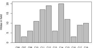
Figure 1: The distribution of Hilda detections in K2 fields. Multiply detected asteroids are multiply counted.

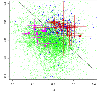
Figure 2: The distribution of Hilda asteroids, detected by SDSS, on the $(r-i)$ - $(i-z)$ color-color diagram. The meaning of the colors are as follows: green: all Main Belt asteroids in SDSS MOC; blue: known Trojans in SDSS MOC; magenta: less red (LR) Hildas observed by K2 and with an entry in SDSS; red: red (R) Hildas observed by K2 and SDSS.

It is suggested that Trojans and outer MB asteroids exhibit different taxonomies (mostly C and X in the outer MB, mostly D and P in the Trojan swarms). Consistently with the dynamical position, D and P type Trojan asteroids, and C and X type outer MB asteroids are also observed in the Hilda group. Wong et al. (2014) suggested a terminology of Red and Less Red Hildas (R and LR, respectively). DeMeo & Carry (2013) defined selection criteria for different taxonomy classes in the $gri$ slope vs. $i-z$ parameter space. According to their criteria, there are C and X asteroids in the LR group, and R Hildas consist mostly P and D types.

Early solar system formation theories stated that Hildas originated in the middle solar system and were captured into their present-day orbits during a period of smooth migration (e.g., Franklin et al., 2004). Current solar system evolution models, however, mostly agree in a scenario in which the gas giants crossed a mutual mean-motion resonance sometime after the era of planet formation, resulting in a notable dynamical restructuring (e.g., Tsiganis et al., 2005; Nesvorný, & Morbidelli, 2012). According to these models many planetesimals which formed in the outer solar system were scattered inward during this period of dynamical instability; in this framework present-day Hildas and Jovian Trojans originate almost exclusively in these populations (Morbidelli et al., 2005; Roig & Nesvorný, 2015).

Gil-Hutton, & Brunini (2008); Roig et al. (2008); Alvarez-Candal (2013); Wong & Brown (2017) and De Prá et al. (2018) studied the color distributions of Hildas and Jovian Trojans and they found them to be consistent with a scenario in which the color bimodality in both populations developed before they were implanted into their present-day orbits. They propose that the shallower magnitude distribution of the Hildas is a result of an initially much larger Hilda population, which was subsequently depleted as smaller bodies were ejected from the narrow 3:2 resonance via collisions, also suggesting a common origin for Hildas and Trojans as predicted by current dynamical instability theories of solar system evolution.

Wong & Brown (2017) investigated the near infrared spectra of Hildas and found that Trojans and Hildas possess similar overall spectral shapes, suggesting that the two minor body populations share a common progenitor population. A more detailed examination reveals that while the red Trojans and Hildas have nearly identical spectra, less-red Hildas are systematically bluer in the visible and redder in the near-infrared than less-red Trojans. They argue that the less-red and red objects found in both Hildas and Trojans represent two distinct surface chemistries and attribute the small discrepancy between less-red Hildas and Trojans to the difference in surface temperatures between the two regions.

Trojans cover a wider range of inclination than the Main Belt, many members going up to 30 degrees inclination, while the eccentricity range of Hildas covers half of that of Trojans, and up to 20 degrees inclination represented by a few members. In essence, Hildas fit more into the Main Belt families in terms of size distribution characteristics; in position their orbits overlap with the Trojan swarms; and taxonomy suggests a region of mixed material of the Trojan swarms and the outer MB.

The comparison of the Trojan and the MB observations shows that there are significant differences between the rotation properties of MBs and Trojans, the average rotation period is lower and the rate of binaries is very high in the Trojan swarms (Szabó et al., 2017). Also, distribution of the minimum density is truncated at a lower value for Trojan asteroids, which is an evidence of significant porosity, in comparison with the MB asteroids. Since the Hilda group is suspected to share the taxonomies of the outer MB and the Trojans, and these large asteroid reservoirs are dynamically coupled via the Hilda group, it is plausible that Hilda asteroids also exhibit a mix of rotation properties of the MB and the Trojan families. It seemed also plausible that the specific rotation properties characteristic to the MB and Trojan asteroids are also preserved in the LR and R group of Hildas, respectively. We investigate this question in this paper, and disproof this simple belief.

The scope of this paper is to provide unbiased period and amplitude distributions of Hilda asteroids, and also, to test differences between the rotational properties of Hildas of Main Belt-like and Trojan-like taxonomy.

2 Observations

The K2 mission observed more than a hundred Hilda asteroids, enabling a detailed analysis of this group. More specifically, trails of 103 Hildas were detected in the K2 Campaigns 6–18. There are multiple detections of 22 Hildas, and in total, there are 125 observations. We did not recover data for 15 objects that were observed in the very crowded stellar fields of Campaigns 7 and 11. The distribution of detected Hilda asteroids is plotted in Fig. 1.

The log of observations is shown in the Appendix (Table 4), listing all detections, and providing separate lines in the case of multiple observations. This is necessary since the observational geometry could have changed significantly, also leading to e.g. the change of light curve amplitude due to the difference aspect angle.

The light curves were extracted by our tools developed to obtain photometry of moving objects in the K2 fields, following the processing scheme developed in Pál et al. (2015, 2016), Kiss et al. (2016), and Molnár et al. (2018). The pipeline is based on the FITSH software package (Pál, 2012). We registered the frames to the same reference system in order to perform differential image analysis. Astrometric solutions were derived for every mosaic frames taken during the campaign using the Full Frame Images (acquired once per campaign) as templates, to register the individual frames. In some cases we also enlarged the images by $\sim 3$ times and transformed them into RA-Dec directions. This subpixel-level re-sampling and spatial transformation helped to decrease the fringing of the residual images in the next step, and, more importantly, allowed us to extract usable light curves for a few targets where the Point Spread Function (PSF) was not fully covered by the pre-selected pixel masks. We then subtracted a median image from all frames in the following way: a series of frames were drawn from the full sample to form a master median-combined image, which was then subtracted from the subsequent frames. The median frame was created from a subset of frames that did not contain the target. We applied simple aperture photometry to the differential images based on the ephemeris provided by the JPL HORIZONS service (Giorgini et al., 1996).

The light curves obtained were analysed with a residual minimization algorithm (Pál et al., 2016; Molnár et al., 2018). In this method we fit the data with a function

$$f(t)~{}=~{}A+B\cos(2\pi f\Delta t)+C\sin(2\pi f\Delta t),$$ (1)

where $f$ is the trial frequency, $\Delta t=T-t$, $T$ the approximate center of the time series, and A, B, and C are fit parameters to be determined. After folding the data with the trial frequency $f$, the dispersion of the folded light curve is calculated in $N\sim 10$ frequency bins as a function of $f$. We search for the minima of the dispersion curves for each frequency. As it is demonstrated in Molnár et al. (2018), the best-fit frequencies obtained with this method are identical to the results of LombScargle periodogram or fast Fourier transform analyses, with a notably smaller general uncertainty in the residuals.

A large fraction of K2 Hilda asteroids were also detected in the Sloan Digital Sky Survey (SDSS). Half of the detections had an entry field in the SDSS Moving Object Catalog (MOC; Ivezić et al., 2001; Jurić et al., 2002; Parker et al., 2008), while the other detections were listed in SDSS PhotoObj files, not recognized as moving targets. The detections were identified using the Solar System Object Image Search facility provided by the Canadian Astronomy Data Centre. After collecting all K2 Hilda detections from SDSS MOC and PhotoObj files, we plotted the color distributions in the $(r-i)$–$(i-z)$ color-color space (Fig. 2). It is seen that Red and Less Red Hildas are convincingly separated (although some asteroids have error bars crossing the suggested boundary).

The measured rotation periods and amplitudes of all Hilda asteroids, and comparison to previous data in the literature is shown in the Appendix (Table 5). The complete collection of light curves, folded light curves and time-frequency distibutions are also shown for all K2 Hilda asteroids in the Appendix.

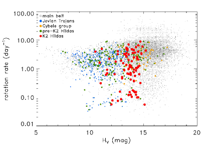
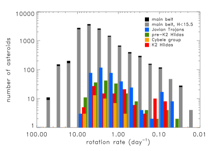
Figure 3: Top: Rotation rate – absolute magnitude distribution of K2 Hilda asteroids (large red dots) compared with Earth-based Hilda observations prior the K2 sample (green dots), Jovian Trojan (blue points), Cybele asteroids (orange dots) and the main belt (gray points). Bottom: The histogram of rotation rates, with the same color coding as in the above panel, but with black and gray bars marking the full main belt sample and the asteroids with H $\leq$ 15.5 mag, respectively. In this plot the sample of Cybele asteroids is restricted to H $\leq$ 15.5 mag, too.

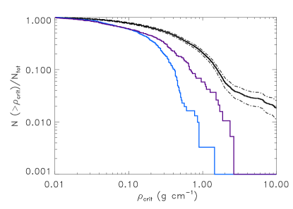
Figure 4: Cumulative number of asteroids with critical densities ($\rho_{crit}$) above a specific value for main belt (black curve, restricted to H_V  15.5 mag), Jovian Trojans (blue) and Hilda asteroids (purple, including both pre-K2 and K2 data). Dash-dotted curves around the main belt (black) curve represent the 1-$\sigma$ confidence intervals.

3 Analysis

In the upper panel of Fig. 3, we plot the rotation rates against the absolute brightness of the observed K2 Hilda asteroids, in comparison with the Main Belt and Trojan asteroids and previous Hilda observations. A similarity is suggested between Hilda and Trojan asteroids, most importantly in the range of very slow rotation. The $P>5$ d (rotation rate $<$0.2 d^-1) wing is populated by many members of both the Hilda and the Jovian Trojan families, and almost completely avoided by Main Belt asteroids. Even, the two samples overlap in the $12<H_{V}<13.5$ where a direct comparison is possible. The K2 sample represents a large number of fainter asteroids, which can appear at higher rotation rates than the larger asteroids, which reflects the size dependence of the break-up velocity. In this sense, Hildas and Jovian Trojans also follow a similar distribution, suggesting a higher porosity of Hilda asteroids. This is again a similarity between Trojan and Hilda asteroids.

In the lower panel of Fig. 3 we compare the spin frequency distribution of Hilda asteroid with that of minor bodies from the main belt and Jovian Trojans. Data for these latter populations, as well as for the pre-K2 Hilda measurements are taken from the Light Curve Database (LCDB, Warner et al., 2009). Cybele asteroids were selected by their osculating orbital elemelents, taken from the Minor Planet Center MPCORB.DAT file, and cross-matched with the Light Curve Database. We required 3.28 au $\leq$ $a$ $\leq$ 3.70 au, $e$ $\leq$ 0.3 and $i$ $\leq$ 25°. Only 39 Cybele asteroids were identified with known rotation periods and absolute brightness below 15.5 mag, making it difficult to draw conclusions from the statistics in this group. For the main belt sample we excluded the data of asteroids families and included minor bodies that were specifically assigned to the main belt (family codes of MB-I, MB-M and MB-O).

The spin frequency distribution of Hildas and Jovian Trojans are similar, with a prominent secondary peak at f $\sim$ 0.1 d^-1, not seen in the main belt population. If a double-Maxwellian distribution is fitted to the full Hilda sample the two peaks of the distribution are at f = 2.5 d^-1 (P = 9.6 h) and f = 2.5 d^-1 (P = 170 h). (Here it has to be noted that the Maxwellian shape is plausible if the group is collosionally relaxed. We do not know this, neither can we test the Maxwellian character of the distribution due to the small sample size. We just consider the Maxwellian fits because they nicely fit the distribution, give a firm statistics for a characteristic rotation period, but do not interpret this fit in the context of dynamical (non) relaxed state.)

Using the definition of slow and fast rotations by Pravec & Harris (2000) the ratio of slow rotators (f $\leq$ 0.8 d^-1) is $>$20 % both among Hildas and Jovian Trojans, notably larger than in the main belt (9.5%, see also Table 1). Similarly, very slow (P $\geq$ 100 h) rotators are also notably abundant in these two resonant populations. A direct comparison is possible in the size range ($H_{\rm V}$=10–14) where all three samples overlap. A factor of 2-3 larger number of slow rotators among K2 Hildas compared with the mostly ground-based Jovian Trojan and pre-K2 Hilda periods show that space surveys with long, uninterrupted time series photometry may more easily detect long period light curves. This has already been the case for the sample of main belt asteroids observed with K2 (Molnár et al., 2018) – the existence of a larger number of slow rotators in the main belt is expected to be confirmed by the TESS Space Telescope due to the longer coverage of uninterrupted observations, and also because the one-day alias periods do not emerge in uninterrupted data, and the period determination will be unique even for very slow rotators (Pál et al., 2018). Therefore, the comparison of the fraction of slow rotators among Trojans, Hildas and the Main Belt must be revisited after the completion of the TESS survey.

Fast rotators (f $\geq$ 7 d^-1) are notably more common in the main belt (13.3%) than among Hildas and Jovian Trojans (2.1 and 0.2%, respectively). In fact, fast rotators are almost completely missing from the Jovian Trojan population. It has to be noted that the Hilda, Trojan and MB samples cover different size ranges in Fig. 3: Trojans down to $H_{\rm V}$=13.5, Hildas down to $H_{\rm V}$=15.5 and MB asteroids down to $H_{\rm V}$=19, and the histogram in Fig 3 lower panel mixes together asteroid samples extending to differing small size limits. The upper panel of Fig. 3 may also suggest that the distribution of fast rotating MB asteroids really extends to higher rotation rates than Hildas and Trojans even at the area where all samples overlap, in the $H_{\rm V}$=13–14.5 range. This was previously explained by the likely low bulk density of these objects (Szabó et al., 2017). Using the rotation periods and light curve amplitudes we calculated the distribution of critical densities in the main belt, Jovian Trojan and Hilda populations (Fig. 4).

To account for the much larger number of main belt asteroids than Hildas and Jovian Trojans in our sample we randomly selected the same number of asteroids from the main belt sample as in the Jovian Trojan sample multiple times, and calculated the mean curve and the $\pm$1$\sigma$ confidence intervals (solid and dash-dotted curve in Fig. 4). The curves indicate a fast extinction of Jovian Trojans – they can be rarely found at $\rho_{crit}$ $>$ 0.5 g cm^-3. Hildas, on the other hand, can easily reach $\rho_{crit}$ $\approx$ 2 g cm^-3, similar to the breakup limit of main belt asteroids. The high density wing of the main belt is not seen in the two resonant populations. The existence of high critical density Hildas has an important implication. While the low critical densities of Jovian Trojans is in agreement with their outer solar system origin (as discussed e.g. Szabó et al., 2017), the $\sim$ 2 g cm^-3 critical density of some Hildas indicate that their building material should be closer to that of main belt asteroids. This suggests a mixed, partly main belt, partly outer solar system, origin of Hildas.

	MB	MB15	JT	Cy.	pre-K2 Hil.	all Hil.	K2 MB	K2 JT	K2 Hil.
N	13072	7874	401	39	187	298	81	56	111
fm [d-1]	3.53	3.95	2.12	2.95	2.63	2.09	3.63	1.76	1.26
Pm [h]	6.79	6.07	11.3	8.11	9.13	11.5	6.60	13.58	19.02
Nf	1930	1057	1	0	7	9	11	2	2
rf [%]	14.8	13.4	0.3	0	3.7	3.0	13.6	3.7	1.8
Ns	1445	908	79	2	29	71	5	14	42
rs [%]	11.1	11.5	19.7	5.1	15.5	23.8	6.2	25.9	37.8
Nvs	488	320	29	0	11	31	0	9	20
rvs [%]	3.7	4.1	7.2	0	5.9	10.4	0	16.7	18.0

Table 1: Summary table of median rotation rates (f_m, and the corresponding period P_m), and the number of slow and fast rotating asteroids in the main belt (MB), Jovian Trojan (JT), Cybele (Cy) and Hilda populations. We defined fast rotators (subscript ’f’) as f $\geq$ 7 d^-1 (P $\leq$ 3.43 h), slow rotators (’s’) as f $\leq$ 0.8 d^-1 (P $\geq$ 30 h) and very slow rotators (’vs’) as f $\leq$ 0.24 d^-1 (P $\geq$ 100 h). The Cybele and Main Belt populations are restricted to H $\leq$ 15.5 mag.

Among Hildas with the longest periods, the typical amplitude is in the 0.4–1.0 magnitude range. As suggested in the case of slowly rotating, high amplitude Trojans (Szabó et al. (2017) and references therein), the high-amplitude, long-period Hilda asteroids can be considered as potential binaries.

Slow rotation of asteroids, however, could also be caused by other effects. This could be, e.g. the disintegration of high mass ratio ($\sim$1:5) binaries through rapid transfer of rotational energy of the primary into the orbit of the secondary due to the irregular shape and gravity field of the primary (Harris, 2002). Small (D $\lesssim$ 20 km) main belt asteroids show a significant deviation from the Maxwellian distribution seen among larger asteroids. This can be well explained by a relaxed YORP evolution (Pravec et al., 2008; Vokrouhlický et al., 2015) for spin rates of f $\approx$ 1–10 d^-1. In this sense Hilda asteroids may also be susceptible to the YORP effect; Hildas in the K2 sample have H_V $\approx$ 10.5–15.5 mag or D $\approx$ 3–40 km. However, in the whole Hilda sample, there are asteroids with slow rotation periods with D $>$ 40 km (H $<$ 10 mag) and the rotation periods in Cluster 3 are notably longer than that explained by the model of Pravec et al. (2008).

Number	$r-i$		$i-z$		Group	P[h]		Amp
1748	0.21$\pm$	0.11	0.14$\pm$	0.05	R	6.	005	0.	09
3655A	0.20$\pm$	0.03	0.20$\pm$	0.03	R	77.	047	0.	19
7394	0.24$\pm$	0.02	0.15$\pm$	0.02	R	4.	836	0.	16
8550	0.11$\pm$	0.04	0.16$\pm$	0.07	LR	37.	209	0.	28
15278	0.28$\pm$	0.02	0.14$\pm$	0.03	R	39.	160	0.	26
15626	0.16$\pm$	0.01	0.10$\pm$	0.02	LR	13.	544	0.	75
16232	0.13$\pm$	0.04	0.03$\pm$	0.05	LR	152.	4	0.	69
16843	0.25$\pm$	0.02	0.18$\pm$	0.04	R	310.	0	0.	28
20628B	0.23$\pm$	0.02	0.18$\pm$	0.03	R	320.	0	0.	95
27561	0.20$\pm$	0.02	0.18$\pm$	0.03	R	—		$<$0.	1
43818	0.21$\pm$	0.03	0.21$\pm$	0.05	R	21.	64	0.	29
46302	0.12$\pm$	0.04	0.08$\pm$	0.05	LR	7.	479	0.	14
51930	0.22$\pm$	0.04	0.19$\pm$	0.02	R	52.	288	0.	37
570271	0.27$\pm$	0.03	0.14$\pm$	0.06	R	4.	800	0.	15
570272	0.27$\pm$	0.03	0.14$\pm$	0.06	R	25.	798	0.	12
60381A	0.21$\pm$	0.02	0.13$\pm$	0.02	R	5.	897	0.	17
78159	0.25$\pm$	0.03	0.18$\pm$	0.06	R	15.	404	0.	22
907041	0.27$\pm$	0.04	0.13$\pm$	0.09	R	4.	760	0.	15
907042	0.27$\pm$	0.04	0.13$\pm$	0.09	R	23.	762	0.	27
92281	0.15$\pm$	0.06	0.10$\pm$	0.11	LR	65.	529	0.	09
98002	0.22$\pm$	0.05	0.08$\pm$	0.1	R	7.	557	0.	25
99276	0.12$\pm$	0.07	0.06$\pm$	0.16	LR	5.	239	0.	07
111995	0.24$\pm$	0.04	0.11$\pm$	0.07	R	—		$<$0.	1
117106	0.11$\pm$	0.05	0.12$\pm$	0.11	LR	32.	090	0.	21
117113	0.15$\pm$	0.03	0.11$\pm$	0.04	LR	136.	908	0.	40
119918	0.12$\pm$	0.02	$-$0.01$\pm$	0.05	LR	5.	006	0.	45
161606	0.30$\pm$	0.06	0.15$\pm$	0.13	R	42.	590	0.	21
1740771	0.33$\pm$	0.06	0.04$\pm$	0.08	R	3.	406	0.	13
1740772	0.33$\pm$	0.06	0.04$\pm$	0.08	R	24.	328	0.	17
174089	0.27$\pm$	0.03	0.10$\pm$	0.05	R	148.	194	0.	86
177943	0.12$\pm$	0.05	0.08$\pm$	0.1	LR	19.	020	0.	27
193449	0.25$\pm$	0.06	0.16$\pm$	0.33	R	21.	111	0.	20
202992	0.28$\pm$	0.06	0.05$\pm$	0.11	R	—		$<$0.	1
207638	0.29$\pm$	0.06	0.07$\pm$	0.13	R	37.	354	0.	28
207644	0.18$\pm$	0.05	$-$0.04$\pm$	0.11	LR	2.	689	0.	23
217032C	0.25$\pm$	0.09	0.22$\pm$	0.16	R	7.	704	0.	42
230294	0.08$\pm$	0.04	0.08$\pm$	0.07	LR	11.	440	0.	57
2362091	0.06$\pm$	0.02	0.07$\pm$	0.04	LR	6.	095	0.	15
2362092	0.06$\pm$	0.02	0.07$\pm$	0.04	LR	18.	480	0.	15
341841	0.16$\pm$	0.04	$-$0.06$\pm$	0.08	LR	4.	030	0.	18

Table 2: SDSS colors, Red (R) / Less Red (LR) group identifications and period, amplitude rotation parameters for K2 asteroids with SDSS counterparts. The remarks in the subscripts are as follows. A: Three humps in the light curve; B: Variable light curve shape, possible tumbler; C: Period and amplitude from Waszczak et al. (2015); 1: First period of a tumbler; 2: Second period of a tumbler.

Hilda asteroids of different taxonomy classes are believed to be of different origin – C and X types are likely related to the main belt while P and D types to the Jovian Trojan swarms – and then evolved as a member of the Hilda group (see e.g. Szabó et al., 2017). A major question related to the present survey was to decide whether the Hildas from different origin preserved the initial rotational properties, or they evolved toward a common distribution, characteristic of Hilda asteroids. Since there are few Hildas with identified R and LR taxonomy in our sample, the direct comparison of the distributions are inconclusive. Instead, we compared the R and LR subset of Hildas to the Trojan and Main Belt samples in our previous K2 publications (Szabó et al., 2017, 2016).

In Table 2, we present the derived periods and amplitudes for those Hildas that had SDSS detections, too (either from MOC, or from our search from the PhotoObj files). Here we give the $r-i$ and $i-z$ color indices, the R/LR classification of the Hildas, and the period and amplitude as involved in the following analysis. (In case of multiple observations, the periods derived in the different campaigns were averaged, and the largest observed amplitude was considered. In case of tumbler asteroids with multiple periods, the shorter period was considered. In the case of 185290, the dominant period in C08 and C13 agree within 2%, although visually C08 is better with three humps, and C13 is better looking with two humps. Since this issue cannot be decided from the current data, we included the two hump solution in the analysis.

In Fig. 5, we plot the LR and R Hildas in the period–amplitude space, in comparison with main belt and Jovian Trojan asteroids in the K2 data. The distribution of R and LR Hildas and Jovian Trojan asteroids are apparently very similar, and we tested this similarity with the energy distance test as described by Székely and Rizzo (2004). This test is a powerful alternative of the Kolmogorov-Smirnov test in arbitrary multiple dimensions, but since it avoids dimension reductions, it preserves the full information. To measure the distance, the data set has to be normalized along the independent dimensions. Hence, we normalized the amplitude in all distributions with the standard deviation of amplitude distribution of the (unified) Hilda asteroids, and the similar recipe for the period was followed, too. The test is evaluated using a so-called jacknife approach, which differs from methods involving the complete bootstrap. Here, only a single pair of random elements from both original samples are chosen and their assignment is commuted. This way, all test samples differ from the original distribution by a split of one single element only. If the samples are different, this change usually decreases the energy distance, because information is lost when distributions of different pattern are mixed together. The test statistics $\alpha$ will be the fraction when changing the single elements led to an increase of the energy distance, therefore significantly differing distributions are characterized by little values of $\alpha$. Székely and Rizzo (2004) suggests that distributions are significantly different when $\alpha<0.1$.

We found that the rotational properties of R type Hilda asteroids differ very significantly from that of Main Belt asteroids ($\alpha$=0.001). Moreover, the rotation properties of Hilda asteroids are seemingly farther from the main belt than that of the Trojans from the main belt (this latter test for different background distribution had a $\alpha$=0.01 value). The period-amplitude distribution of LR type Hildas is likely distinguishable from Main Belt asteroids ($\alpha$=0.05), but indistinguishable from Trojans. Also, the unified sample of all Hildas is indistinguishable from the Trojans by rotation properties in a direct comparison.

This comparison results in a somewhat surprising picture. The R group of Hilda asteroids (D and P type for taxonomy) follows a similar period and amplitude distribution as the Jovian Trojans, which is an indication of their origin from the Trojan swarms, and that later they preserved the initial rotation properties. On the other hand, the period and amplitude distributions of the LR group (mostly C and X type) Hilda asteroids also resemble that of the Trojan asteroids, and not the main belt. This can either mean that (1) there is a recognisable distribution of rotation periods and amplitudes in the Hilda group, and all asteroids evolved to this distribution by now, regardless of their origin; and this distribution is close to that of the Jovian Trojans; or (2) all types of Hilda asteroids could preserve their original rotation properties, but the LR type Hildas originated from a part of the outer Main Belt where the rotation amplitudes and periods were unlike in the major part of the Main Belt, but very close to the Jovian Trojans instead; (3) the K2 observations of Main Belt asteroids covered a shorter average time span and is truncated for very slow rotation periods, preventing us from directly comparing the K2 Hildas and Trojan asteroids. The answer has to be postponed to later surveys such as the Solar System objects in TESS data, or the LSST.

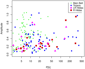
Figure 5: The distribution of LR and R groups of K2 Hilda asteroids, compared to the K2 sample of Main Belt and Trojan asteroids.

3.1 Hilda asteroids with double periods

In the K2 sample we found an unusually high ratio of asteroids with double periods. Similar observations of double periods are usually interpreted as an outcome of a double asteroid, or a single asteroid in the state of tumbling (Paolicchi et al., 2002).

Asteroid tumbling is explained by the misalignment of the axis of instantaneous rotation and the angular momentum vector. Therefore, the axis of the instantaneous rotation traces the herpolhodie cone (with the axis of symmetry being the angular momentum vector), and the axis of maximal inertia ($c$ axis in the triaxial shape approximation of the body shape) traces along the nutation cone (whose axis of symmetry is also the angular momentum vector, but the cone angle can be different). Thus, the body can be interpreted as rotating around two axes, and two periods are observed in the light curves.

Asteroid tumbling is damped by tidal forces from distant bodies and internal stress waves (Paolicchi et al., 2002). The tumbling state of a free Solar System body ceases in the time scale of $10^{5}$ yr, and is considered to be a transient state of rotation. Tumbling can be straightforwardly triggered by an energetic impact between asteroids. It has to be noted that the YORP effect can also excite tumbling, and since YORP can act continuously, this kind of tumbling does not decay (decays or excites slowly together with the YORP induced evolution of the rotation axis (Slivan et al., 2009)).

Another usual reason of a second period is a large companion around the asteroid. We can observe the rotation of the two bodies as two periods in the light curve if the companion is not much smaller than the primary body.

In the case of the tumbling, the period ratio depends on the moments of inertia, the period ratio equals $\sqrt{(\Omega_{3}/\Omega_{1}-1)(\Omega_{2}/\Omega_{1}-1)}$. From the large size and the low observed amplitude (0.12–0.17) of the Hilda asteroids with double periods, likely $\Omega_{\rm 2,3}$ are close to $\Omega_{\rm 1}$, and the ratio of the rotation and precession periods are predicted to differ significanlty. Indeed, the observed period ratios are roughly 3, 5 and 7.2 for asteroids 236209, 90704 and 174077, respectively, which is compatible with tumbling.

The binarity scenario cannot be excluded either, because the fast signal in the light curves can be considered as the rotation of the main body, while the period of the slow signals are compatible with the bound revolution of a companion. Most importantly, in the case of 236209 and 90704, where the period ratios are very close to integers 3 and 5, respectively, pointing towards a possible spin-orbit resonance.

In the case of a very long period asteroid (20628) 1999 TS40, P$\approx$320 h, only two rotation cycles were observed, but the notable light curve variations are characteristic of a tumbler asteroid. The tumbling nature of (20628) 1999 TS40 was first proposed by Pravec et al. (2005), later debated by Pravec et al. (2014) but confirmed by (Warner & Stephens, 2018). The long period continuous light curve of K2 proves the long time systematic light curve variations, as an evidence for tumbling.

All tumblers have been identified in SDSS (90704 1988 RO12, 174077 2002 FP21, and 236209 2005 WT122, besides of the above discussed 20628 1999 TS40). Of the tumblers, (236209) 2005 WT122 is the only LR-type Hilda asteroid, while the three other tumblers belong to the R group.

We identified one asteroid, (57027) 2000 UB59, that is most likely an asynchronous binary, i.e., a larger primary with a small companion, and the rotation of the larger component has not synchronised with the orbital period. The light curve of 57025 shows both a fast, rotation-like signal ($P_{rot}=4.80$ h), and a longer variation characterized by short, distinct eclipses, with a maximal depth of 0.12 mag ($P_{orb}=25.80$ h).

3.2 Hilda asteroids with triple light curve symmetry

In the K2 Hilda sample, we found 4 asteroids exhibiting a trimodal light curve with three humps (three minima and three maxima) during one rotation: 1748, 3655, 60381, 249182. (We note that C08 observations of 185290 can also be better interpreted as three humps with 85 h rotation period, while C13 observations are more symmetric, can be compatible with either 57.5 or 85.3 h period.) Majority of light curves with two minima/maxima in one cycle can be well fitted with a rotating ellipsoid, but these trimodal light curves represent a prominent deviation from the usual case. The simplest shape that can be seen to generate a trimodal light curve is a tetrahedron with an inclined aspect of the rotation angle and/or phase angle of incident light. Such shape is not necessarily built up by mergers, but a merger outcome can be similar. Therefore, the large fraction of light curves with three humps can also be a sign of a significant fraction of binary asteroids and merged asteroids in the Hilda group.

3.3 Hilda asteroids with very long periods

As presented in Fig 3 and Table 1 the Hilda period distribution has a very heavy wing towards long periods. Indeed, the distribution (Fig. 3) indicates that a notable characteristic of the rotation properties is the surprisingly large fraction of long-period Hilda asteroids. About 38% of K2 Hildas have $P_{\rm rot}$ $\geq$ 30 h, and 18% of Hildas reside in the $P_{\rm rot}>$100 h regime. A similar overpopulation of slow rotators was observed in the Jovian Trojan K2 sample. On the contrary, none of the 120 Main Belt K2 asteroids showed a rotation period above 100 h (see also Table 1.).

In Szabó et al. (2017) we concluded that the Trojan swarms contain a considerable fraction of unusual asteroids – slow rotators, tumblers and trimodal light curves – implying a large number of binaries in the Trojan swarms. Although the rotation periods and amplitudes are very similar in the case of Hilda and Trojan asteroids, it is interesting that the ratio of unusual asteroids is even larger in the Hilda group than in the Trojan swarms, the most significant difference is the rich population of long period asteroids especially in the case of very slow rotators ($P>100$ h) in the Hilda group which is true in total numbers, Fig. 3. lower panel, and also true in the overlapping size region, Fig. 3 upper panel. These findings suggest a general similarity of Trojan and Hilda asteroids for dynamical properties, but, interestingly, the binary fraction in the Hilda group is likely even larger than in the Trojan swarms. The same was concluded by Sonnett et al. (2015) from NEOWISE data, which we confirm from K2 observations. At least from this aspect, the Hilda group is not an intermediate mix between the Trojans and the Main Belt, but it represents the end of the range.

4 Summary

In this paper we analysed 125 individual light curves of Hilda asteroids from the K2 mission, and concluded the following results.

• The period-amplitude distribution of Hilda asteroids is very similar to the Trojan populations. In fact, rotation properties of Hildas and Trojans are statistically indiscernible.

• The rotation parameters of Hildas are distinctly different from that of the Main Belt, as there are only a low number of fast rotator Hildas, however, this ratio in even lower for the Jovian Trojans. This is also true for LR type Hildas, although they are expected to originate from the Main Belt.

• Both Hilda subgroups with Trojan-like (R group, D and P) and Main Belt-like (LR group, C and X) taxonomy share very similar rotation properties.

• The median rotation period of K2 Hilda asteroids is 20.7 hours, the mean period is 54.8 hours. Both values prominently exceed that of the known Main Belt asteroids. There is an unprecedentedly large fraction ($\approx$ 18%) of extreme slow rotators ($P$ $>$ 100 h).

• We found 4 asteroids with double periods, where binarity is the most reasonable explanation in 2 cases. The other 2 cases can be a result of either binarity or tumbling.

• We identified 5 asteroids with three maxima in the light curve.

• We found that the binarity rate of Hildas is among the highest in the asteroid belt, likely exceeding that of the Trojan swarms, too.

Table 3: Hilda asteroids observed by K2, ordered by the campaign of the observation. The columns are: (1) the number and name/designation; (2) the reference to the K2 campaign when the asteroid was observed; (3-4) start and end date in Julian Date; (5) the length of obervations in days, (6) the number of frames where the asteroid was detected; (7) the duty cycle of the observations (ratio of useful cadences and all cadences over the time span of the observations); (8) the $r$ heliocentric distance in AU; (9) $\Delta$ K2–object distance in AU; (10) the phase angle of the observation from K2.

Name	Cam.	Start	End	Length	#frame	Duty	$r$	$\Delta$	$\alpha$
(113224) 2002 RN121	C06	2457220.6050	2457230.9648	10.360	481	0.946	4.242…4.255	3.469…3.570	10.342…11.887
(15626) 2000 HR50	C06	2457262.4121	2457270.3199	7.908	337	0.868	4.308…4.312	4.163…4.280	13.962…14.061
(3655) Eupraksia	C06	2457233.2534	2457253.1966	19.943	663	0.678	4.729…4.741	4.077…4.330	10.600…12.303
(39301) 2001 OB100	C06	2457261.1452	2457271.5459	10.401	434	0.850	4.397…4.413	4.128…4.263	13.555…13.738
(46302) 2001 OG13	C06	2457282.1510	2457293.0217	10.871	453	0.849	3.678…3.700	3.881…3.999	14.756…15.543
(51930) 2001 QW127	C06	2457217.4582	2457228.3289	10.871	506	0.949	4.204…4.221	3.426…3.530	10.288…11.977
(78159) 2002 NA28	C06	2457223.4861	2457229.6571	6.171	274	0.904	4.487…4.491	3.741…3.806	10.256…11.085
(8550) Hesiodos	C06	2457280.5163	2457288.3219	7.806	355	0.926	4.696…4.706	4.895…4.995	11.783…12.247
(99276) 2001 QC20	C06	2457226.9598	2457247.0052	20.045	925	0.941	3.926…3.964	3.239…3.452	12.153…14.605
(185290) 2006 UB219	C08	2457405.2838	2457434.3608	29.077	1256	0.881	4.255…4.288	3.585…3.960	10.010…9.969
(202992) 1999 VG135	C08	2457392.0633	2457412.4356	20.372	371	0.371	2.751…2.760	1.955…2.164	13.912…18.436
(203157) 2000 WC140	C08	2457392.0633	2457418.3818	26.319	1128	0.875	3.194…3.241	2.448…2.721	11.805…16.667
(20628) 1999 TS40	C08	2457394.4949	2457426.5143	32.019	1475	0.940	3.171…3.204	2.377…2.720	10.995…16.955
(20630) 1999 TJ90	C08	2457392.0633	2457416.5019	24.439	1188	0.992	2.884…2.900	2.083…2.338	12.752…17.936
(402869) 2007 RY194	C08	2457393.8001	2457427.1069	33.307	1595	0.977	3.436…3.445	2.632…3.035	10.482…15.849
(148227) 2000 DP99	C10	2457582.5862	2457589.3701	6.784	317	0.951	3.497…3.505	2.781…2.864	14.038…15.033
(152133) 2004 TN126	C10	2457582.5862	2457612.9914	30.405	570	0.383	4.098…4.111	3.386…3.791	11.804…14.543
(16232) Chijagerbs	C10	2457603.7962	2457609.5381	5.742	278	0.985	3.702…3.707	3.199…3.276	15.381…15.785
(177943) 2005 VZ17	C10	2457582.5862	2457589.7788	7.193	343	0.971	3.532…3.539	2.857…2.946	14.443…15.366
(341841) 2008 DN52	C10	2457582.5862	2457589.7788	7.193	340	0.963	3.565…3.574	2.806…2.892	13.063…14.198
(43818) 1992 ET32	C10	2457582.5862	2457607.8830	25.297	544	0.439	3.492…3.503	2.723…3.029	13.207…16.535
(90704) 1988 RO12	C10	2457584.6500	2457605.9622	21.312	297	0.284	3.931…3.937	3.335…3.624	13.633…15.240
(99281) 2001 QR99	C10	2457582.5862	2457589.7788	7.193	339	0.960	1.872…1.877	1.436…1.506	33.695…33.872
(30764) 1981 EK47	C12	2457738.3719	2457770.6570	32.285	1531	0.968	4.476…4.485	3.657…4.069	10.005…9.970
(58279) 1993 TE40	C12	2457738.3719	2457747.5057	9.134	421	0.939	4.276…4.284	3.480…3.574	10.032…9.992
(16843) 1997 XX3	C12	2457743.4394	2457759.3572	15.918	597	0.765	3.535…3.558	2.794…3.013	12.010…14.380
(16915) 1998 FR10	C12	2457756.0061	2457771.1065	15.100	733	0.990	4.135…4.153	3.474…3.700	11.070…12.736
(31338) 1998 HX147	C12	2457779.7295	2457786.1048	6.375	274	0.875	4.193…4.195	3.862…3.960	13.131…13.364
(65989) 1998 KZ12	C12	2457743.6846	2457767.1628	23.478	1014	0.881	4.444…4.461	3.702…4.038	10.022…9.986
(98002) 2000 QG199	C12	2457748.7522	2457763.7096	14.957	705	0.961	3.923…3.944	3.228…3.444	11.336…13.179
(76811) 2000 QK57	C12	2457753.1658	2457768.0006	14.835	622	0.855	4.192…4.198	3.544…3.756	11.073…12.657
(130453) 2000 QT59	C12	2457763.9343	2457778.5239	14.590	677	0.946	3.727…3.746	3.209…3.439	13.859…14.870
(77893) 2001 SM251	C12	2457740.3335	2457754.3306	13.997	665	0.969	3.893…3.905	3.077…3.245	10.011…9.963
(131502) 2001 SW273	C12	2457743.7255	2457759.0303	15.305	703	0.937	3.717…3.739	2.993…3.211	11.645…13.769
(77892) 2001 SZ250	C12	2457760.8693	2457775.7858	14.917	714	0.976	4.515…4.523	3.911…4.116	10.492…11.907
(83801) 2001 TG218	C12	2457738.3719	2457766.8768	28.505	1223	0.875	3.978…4.027	3.220…3.539	10.019…9.971
(83722) 2001 TL98	C12	2457750.3869	2457772.2917	21.905	1036	0.965	4.441…4.451	3.725…4.036	10.009…9.973
(77903) 2001 TQ142	C12	2457769.6149	2457774.5189	4.904	218	0.904	4.543…4.544	4.127…4.200	11.773…12.051
(55505) 2001 UK113	C12	2457738.3719	2457772.0465	33.675	1596	0.967	4.472…4.473	3.632…4.063	10.020…9.985
(90456) 2004 CV2	C12	2457765.6099	2457780.5264	14.916	367	0.502	4.479…4.492	3.896…4.100	10.703…12.078
(216411) 2008 RR51	C12	2457741.0487	2457751.2655	10.217	486	0.969	3.664…3.674	2.832…2.950	10.038…9.983
(7394) Xanthomalitia	C12	2457746.9336	2457761.9931	15.059	727	0.984	3.802…3.803	3.108…3.307	11.760…13.752
(193354) 2000 UX34	C13	2457830.4866	2457850.5524	20.066	505	0.513	3.247…3.276	2.484…2.746	12.512…16.050
(193449) 2000 WW146	C13	2457822.1701	2457837.0662	14.896	673	0.921	2.670…2.692	1.889…2.063	15.147…18.503
(195204) 2002 CR306	C13	2457835.2272	2457849.8576	14.630	642	0.895	3.461…3.480	2.742…2.936	12.531…14.896
(185290) 2006 UB219	C13	2457831.2835	2457846.3022	15.019	561	0.762	3.832…3.844	3.183…3.368	11.931…13.967
(403237) 2008 VE11	C13	2457826.5429	2457841.5820	15.039	677	0.918	2.825…2.835	2.046…2.215	14.255…17.621
(19034) Santorini	C13	2457830.8339	2457845.7096	14.876	647	0.887	3.136…3.157	2.379…2.567	13.189…16.012
(1748) 1951 XD	C14	2457929.8960	2457941.8905	11.995	579	0.984	4.699…4.708	4.131…4.283	11.205…12.221
(13035) 1977 CE2	C14	2457926.4836	2457936.9660	10.482	509	0.990	3.981…3.995	3.353…3.469	12.734…13.984
(7174) 1988 SQ	C14	2457928.9356	2457938.0899	9.154	444	0.988	4.168…4.181	3.566…3.670	12.392…13.407
(120962) 1998 VM11	C14	2457925.2167	2457937.2725	12.056	560	0.947	4.635…4.640	4.038…4.205	11.200…12.274
(134652) 1999 VT37	C14	2457923.4186	2457935.5357	12.117	514	0.865	4.586…4.603	3.981…4.159	11.250…12.328
(60381) 2000 AX180	C14	2457924.1542	2457935.0044	10.850	515	0.967	4.401…4.409	3.737…3.865	11.097…12.387
(86435) 2000 CL9	C14	2457929.3034	2457939.7654	10.462	488	0.951	4.227…4.236	3.605…3.727	12.073…13.205
(18916) 2000 OG44	C14	2457930.1821	2457946.6516	16.470	670	0.830	4.196…4.271	3.581…3.874	12.359…13.626
(208290) 2001 DH1	C14	2457920.7622	2457927.6892	6.927	324	0.952	4.056…4.064	3.419…3.496	12.413…13.284
(63293) 2001 DT89	C14	2457923.6025	2457935.6992	12.097	554	0.934	4.132…4.147	3.516…3.657	12.305…13.657
(174074) 2002 EO133	C14	2457925.9932	2457938.0082	12.015	518	0.879	4.285…4.304	3.697…3.838	12.060…13.300
(174077) 2002 FP21	C14	2457930.1208	2457941.4819	11.361	541	0.971	4.138…4.151	3.565…3.702	12.767…13.878
(146961) 2002 GH129	C14	2457921.4978	2457933.5945	12.097	406	0.684	3.765…3.780	3.101…3.234	13.053…14.688
(119942) 2002 GJ129	C14	2457925.1963	2457937.2725	12.076	513	0.866	4.229…4.239	3.609…3.755	12.039…13.338
(174089) 2002 GX137	C14	2457927.7505	2457939.7859	12.035	547	0.927	3.641…3.657	2.962…3.089	13.390…15.118
(141557) 2002 GY69	C14	2457923.3981	2457935.3518	11.954	504	0.859	3.743…3.754	3.065…3.195	13.032…14.665
(177640) 2003 JF14	C14	2457925.9728	2457938.0899	12.117	579	0.974	4.637…4.651	4.079…4.230	11.360…12.410
(117113) 2004 PG11	C14	2457931.0199	2457943.0553	12.035	397	0.672	4.294…4.301	3.676…3.826	11.945…13.189
(207644) 2006 UW322	C14	2457923.4594	2457935.5561	12.097	557	0.939	3.734…3.734	3.029…3.172	12.901…14.587
(39415) Janeausten	C14	2457929.6304	2457936.3122	6.682	323	0.984	4.189…4.199	3.651…3.728	12.899…13.540
(90704) 1988 RO12	C15	2458005.4390	2458020.5395	15.101	612	0.826	4.031…4.034	3.301…3.490	11.814…13.621
(11274) 1988 SX2	C15	2458007.7480	2458021.5611	13.813	502	0.741	4.805…4.806	4.181…4.370	10.754…11.866
(7284) 1989 VW	C15	2458010.0979	2458024.9940	14.896	688	0.942	4.581…4.588	3.915…4.118	10.924…12.274
(178295) 1992 DJ6	C15	2458008.9127	2458024.0336	15.121	595	0.802	4.214…4.232	3.498…3.705	11.406…13.038
(152900) 2000 DC27	C15	2457999.4724	2458014.6137	15.141	608	0.819	4.112…4.131	3.387…3.592	11.642…13.352
(92283) 2000 DC45	C15	2457997.7151	2458012.7134	14.998	462	0.628	3.739…3.746	2.970…3.150	12.290…14.360
(29053) 2000 DL95	C15	2458006.1338	2458021.1525	15.019	656	0.891	4.045…4.053	3.315…3.509	11.773…13.555
(176158) 2001 HG21	C15	2457998.6755	2458013.7759	15.100	692	0.935	3.677…3.686	2.903…3.086	12.426…14.571
(114954) 2003 QE57	C15	2458008.5858	2458023.5636	14.978	564	0.768	4.295…4.327	3.675…3.840	11.788…13.260
(147836) 2005 TN125	C15	2458000.3919	2458015.4719	15.080	567	0.767	3.889…3.908	3.137…3.337	12.009…13.911
(161606) 2005 UR38	C15	2458001.6792	2458016.7388	15.060	594	0.804	4.215…4.217	3.515…3.705	11.600…13.241
(249182) 2008 CW119	C15	2458004.1721	2458019.1704	14.998	642	0.873	3.712…3.723	2.946…3.130	12.398…14.448
(62489) 2000 SS223	C16	2458157.8941	2458167.1505	9.256	330	0.726	3.210…3.217	2.494…2.596	13.328…15.148
(87956) 2000 TM4	C16	2458149.9046	2458160.8366	10.932	494	0.921	3.175…3.189	2.487…2.603	13.868…15.889
(194512) 2001 XR	C16	2458148.9646	2458159.3449	10.380	311	0.611	3.479…3.495	2.838…2.955	13.205…14.828
(1748) 1951 XD	C17	2458200.7434	2458210.8171	10.074	475	0.961	4.386…4.401	4.054…4.226	12.640…12.867
(233980) 1995 NF1	C17	2458219.7875	2458240.8341	21.047	911	0.883	3.824…3.866	3.074…3.387	11.105…13.751
(120962) 1998 VM11	C17	2458208.3242	2458229.3300	21.006	844	0.820	4.647…4.653	3.986…4.297	10.015…9.984
(119918) 2002 EX84	C17	2458237.7486	2458246.5759	8.827	420	0.969	3.609…3.621	2.797…2.905	10.694…12.346
(111995) 2002 GG114	C17	2458207.2821	2458220.9522	13.670	610	0.910	4.363…4.372	3.909…4.124	12.237…12.884
(117106) 2004 OT6	C17	2458219.7875	2458240.8954	21.108	722	0.698	4.099…4.112	3.375…3.670	10.676…13.100
(236209) 2005 WT122	C17	2458217.8463	2458238.9133	21.067	936	0.906	4.087…4.110	3.369…3.677	10.775…13.139
(207638) 2006 TJ32	C17	2458217.2741	2458238.3616	21.087	808	0.782	3.930…3.942	3.194…3.484	10.968…13.586
(237323) 2009 BP88	C17	2458226.8575	2458245.7382	18.881	796	0.860	3.835…3.850	2.985…3.209	10.010…9.960
(58353) 1995 EW4	C18	2458253.3190	2458273.8548	20.536	879	0.873	3.772…3.803	2.993…3.261	10.942…14.121
(193241) 2000 ST33	C18	2458255.3011	2458276.3068	21.006	963	0.935	3.448…3.498	2.685…2.979	12.485…15.691
(36941) 2000 SV239	C18	2458257.7531	2458278.7180	20.965	923	0.898	3.661…3.682	2.919…3.189	12.068…15.054
(57027) 2000 UB59	C18	2458256.6497	2458277.7167	21.067	928	0.899	3.655…3.677	2.912…3.187	12.068…15.083
(45862) 2000 UQ51	C18	2458282.3756	2458297.8030	15.427	706	0.933	4.080…4.101	3.585…3.818	13.492…14.446
(270356) 2001 YU49	C18	2458251.5413	2458270.8306	19.289	861	0.911	3.143…3.171	2.379…2.621	13.804…17.114
(230294) 2001 YW79	C18	2458258.3252	2458279.2697	20.945	981	0.956	3.700…3.732	2.965…3.248	12.038…14.896
(274543) 2008 SJ248	C18	2458259.1221	2458277.2468	18.125	789	0.888	3.316…3.339	2.554…2.779	13.147…16.150
(2483) Guinevere	C18	2458251.5413	2458270.4219	18.881	846	0.914	3.231…3.272	2.478…2.731	13.598…16.610
(15278) Paquet	C18	2458259.6330	2458275.6121	15.979	718	0.916	3.792…3.822	3.095…3.318	12.297…14.344

Table 4: Periods of K2 Hildas, ordered by the asteroid numbers. The columns are: (1) the number of the asteroid; (2) the campaign of the observation; (3) observation in SDSS, the number of detections in parenthesis; (4) sinodical rotation period in days; (5) peak-to-peak amplitude in magnitude; (6) period and amplitude in previous publications, and the reference; (7) remarks. For Hildas which were detected in multiple campaigns we derived the period and the amplitude for each campaigns separately.

Number	Campaign	SDSS	Period (d)	Amplitude (mag)	Values in prev. publ.	Remarks
1748	C14	yes (1)	6.005	0.09	6.00, 0.12 (Dahlgren 1998)	three humps
	C17	yes (1)	6.000	0.07	6.001, 0.1 (Slyusarev 2012)	three humps
					5.552, 0.25 (Warner 2017c)
					5.320, 0.08 (Warner 2018c)
					5.551, 0.23 (Warner 2018c)
2483	C18	yes (2)	14.733	1.38	14.733, 1.38 (Dahlgren 1998)
					14.731, 1.37 (Durech 2016)
					14.730, 0.89 (Warner 2017b)
					14.721, 1.37 (Warner 2018a)
3655	C06	yes (1)	77.047	0.19	>20, 0.07 (Dahlgren 1998)	three humps
					75.668, 0.23 (Waszczak 2015)
7174	C14	no	34.433	0.13	7.456, 0.38 (Warner 2017c)
7284	C10	no	26.17	0.08
	C15	no	26.42	0.08
7394	C12	yes (3)	4.836	0.16
8550	C06	yes (2)	37.209	0.28	6.719, 0.09 (Warner 2019)
11274	C15	no	158.940	0.86
13035	C14	yes	10.660	0.44	10.657, — (Durech 2016)
					10.639, 0.57 (Warner 2018c)
15278	C18	yes (1)	39.160	0.26	40.01, 0.41 (Warner 2017a)
15626	C06	yes (9)	13.544	0.75	13.277, 0.68 (Waszczak 2015)
16232	C10	yes (1)	152.400	0.69
16843	C12	yes (2)	309.5	0.28	275, 0.41 (Warner 2017a)
16915	C12	no	425.155	0.95		very long per.
18916	C14	no	22.493	0.18
19034	C13	no	280.784	0.79	247, 0.43 (Warner 2017b)
20628	C08	yes (2)	320.0	0.95	68.1, 1.04 (Warner 2018b)	tumbler
20630	C08	no	25.750	0.43
27561	C11	yes (1)	—	<0.1		no signal
29053	C15	no	17.980	0.24
30764	C12	yes (2)	24.930	0.41
31338	C12	no	7.670	0.18
36941	C18	no	36.954	0.21
39301	C06	no	12.572	0.42
39415	C14	no	7.317	0.62
43818	C10	yes (3)	21.640	0.29
45862	C18	yes (1)	13.159	1.00
46302	C06	yes (1)	7.479	0.14
51930	C06	yes (1)	52.288	0.37
55505	C12	no	4.460	0.25
57027	C18	yes (4)	4.800	0.15		rotation
			25.798	0.12		orbit
58279	C12	no	6.836	0.18
58353	C18	no	156.550	0.53
60381	C14	yes (6)	5.897	0.17	28.96, 0.30 (Warner 2018c)	three humps
62489	C16	yes (1)	63.583	0.58
63293	C14	no	199.68	0.53
65989	C12	yes (1)	35.357	0.05
76811	C12	yes (2)	26.754	0.15
77892	C12	no	26.388	0.26
77893	C12	no	6.028	0.09
78159	C06	yes (5)	15.404	0.22
83722	C12	yes (1)	9.074	0.65
83801	C12	no	18.721	0.05
86435	C14	no	47.0	0.08
87956	C16	yes (2)	160.6	0.49
90456	C12	yes (3)	17.622	0.12
90704	C10	yes (1)	4.760	0.15		tumbler P1
			23.762	0.27		tumbler P2
	C15	yes (1)	4.735	0.16
92281	C10	yes (4)	65.529	0.09
92283	C15	no	5.490	0.29
92284	C10	no	6.800	0.10
98002	C12	yes (1)	7.557	0.25
99276	C06	yes (2)	5.239	0.07
111995	C17	yes (1)	—	—		no signal
113224	C06	no	8.624	0.35
114954	C15	no	39.216	0.32
117106	C17	yes (1)	32.090	0.21
117113	C14	yes (6)	136.908	0.40
119918	C17	yes (8)	5.006	0.45
119942	C14	no	5.120	0.52	5.119, 0.51 (Waszczak 2015)
120962	C14	no	37.134	0.16
	C17	no	34.593	0.18
130453	C12	yes (1)	230.7	0.36
131502	C12	yes (1)	195.4	0.66
134652	C14	no	33.932	0.21
141557	C14	yes (1)	9.636	1.02
146961	C14	no	243.7	0.66
147836	C15	no	240.0	0.73
148227	C10	no	6.795	0.03		small amplitude
152133	C10	no	5.174	0.27
152900	C15	no	10.530	0.77
161606	C15	yes (1)	42.590	0.21
174074	C14	no	43.015	0.16
174077	C14	yes (1)	3.406	0.13		tumbler P1
	C14	yes (1)	24.328	0.17		tumbler P2
174089	C14	yes (5)	148.19	0.86
176158	C15	no	194.4	0.62
177640	C14	no	11.939	0.20
177943	C10	yes (6)	19.020	0.27
178295	C15	no	6.581	0.19
185290	C08	no	85.318	0.15		three humps
	C08	no	56.878	0.15		dominant period
	C13	no	57.554	0.09
193241	C18	yes (1)	4.203	0.06
193354	C13	yes (1)	27.6	0.08
193449	C13	yes (3)	21.111	0.20	38.44, 0.20 (Warner 2017b)
194512	C16	yes (1)	76.286	0.30
195204	C13	yes (1)	9.326	0.18
203157	C08	no	6.895	0.79
207638	C17	no	37.354	0.28
207644	C14	yes (5)	2.689	0.23
208290	C14	no	3.643	0.36
216411	C12	yes (4)	22.555	0.95
230294	C18	yes (2)	11.440	0.57
233980	C17	no	20.739	0.32
236209	C17	yes (11)	6.095	0.15		tumbler P1
	C17	yes (11)	18.48	0.15		tumbler P2
237323	C17	no	5.375	1.08
249182	C15	no	9.364	0.09		three humps
270356	C18	yes (1)	20.293	0.16
274543	C18	no	432.2	0.81		very long per.
341841	C10	yes (5)	4.030	0.18
402869	C08	no	7.260	0.82
403237	C13	no	5.597	0.24

Fig. Set6.

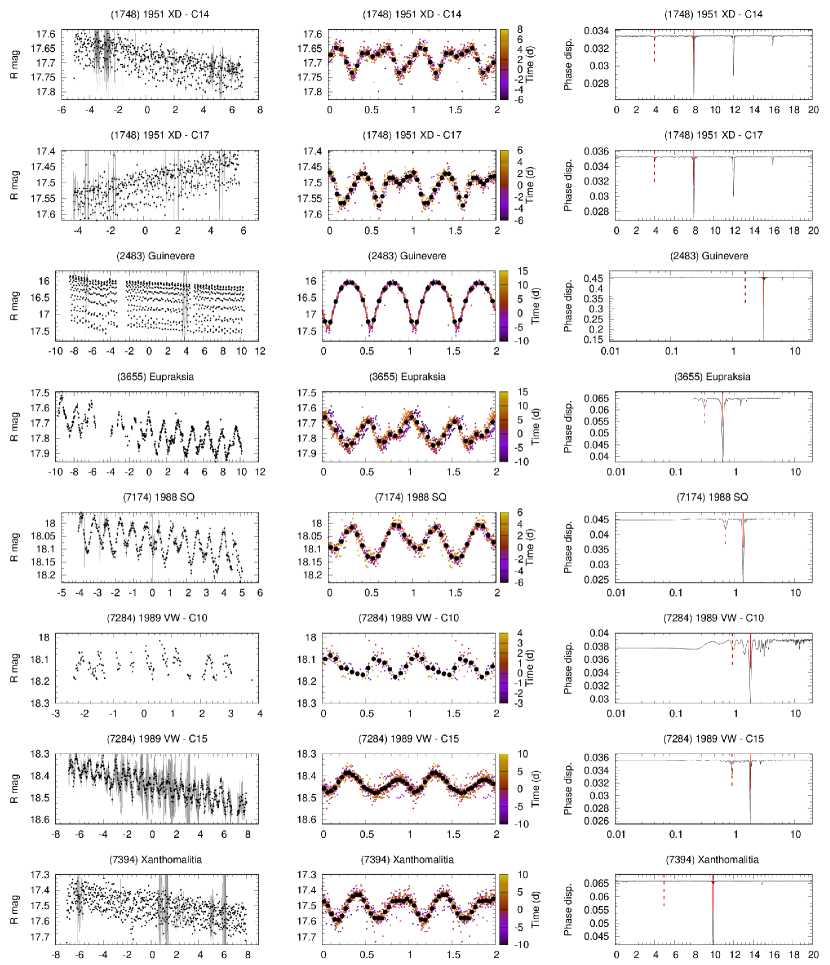
Figure 6: Light curves of Hildas observed by K2. Left: raw light curves. Middle: rectified and folded phase curves. Dots are phase-binned points, color shows time. Right: residual dispersion frequency spectra. Red solid and dashed lines mark frequencies for the single- and double-peak solutions.

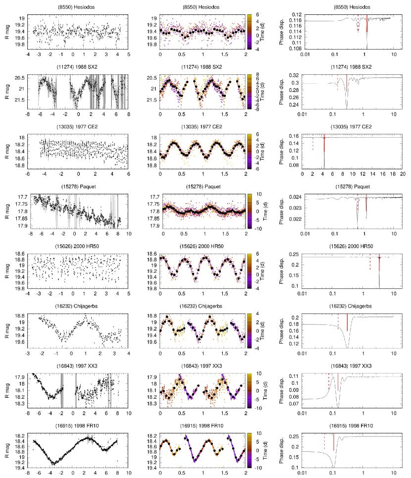
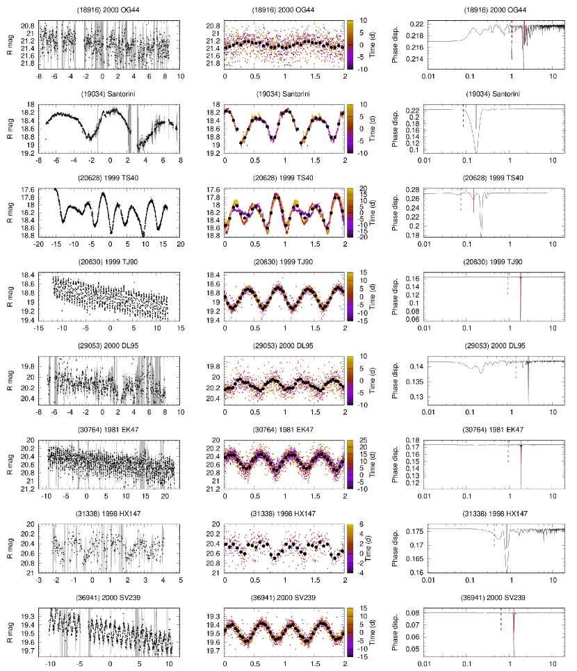
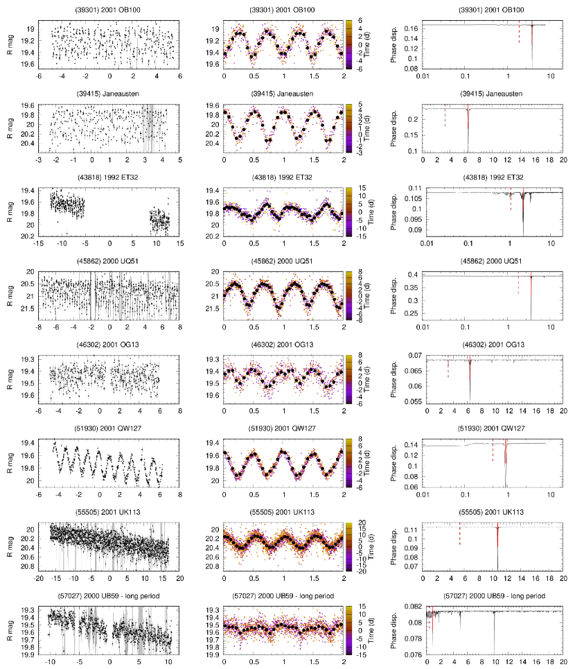
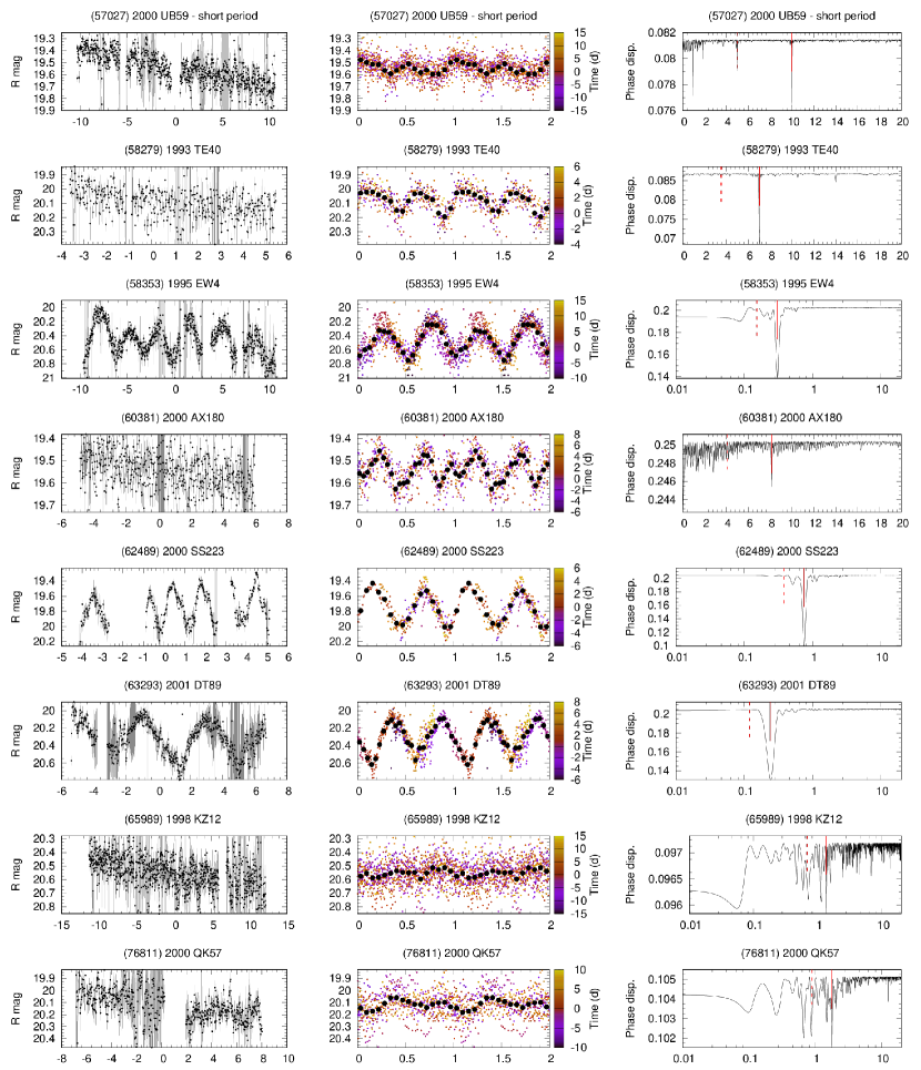
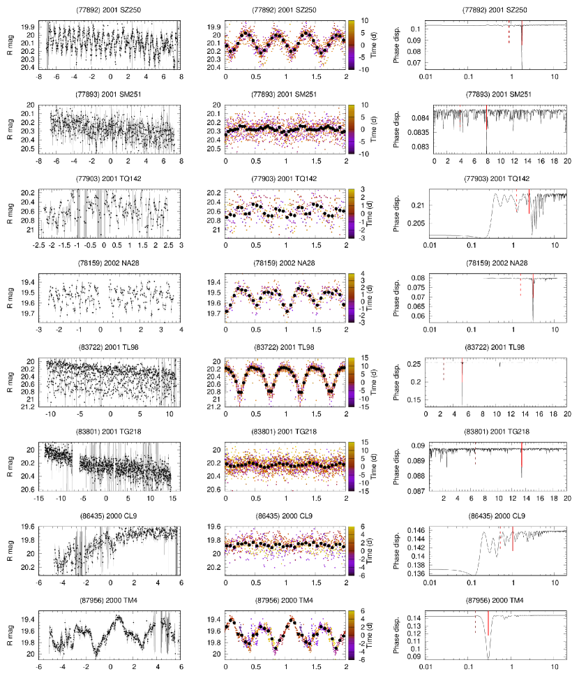
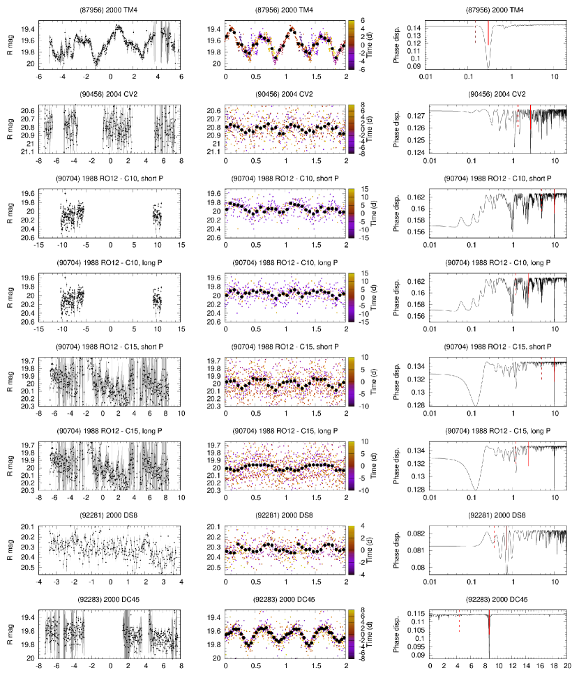
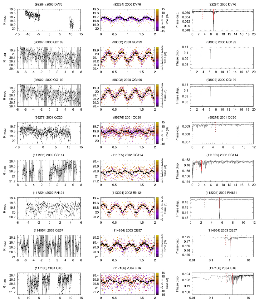
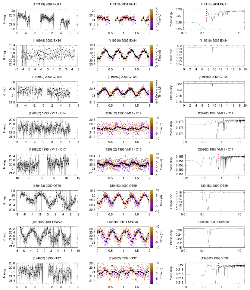
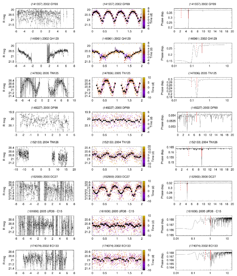
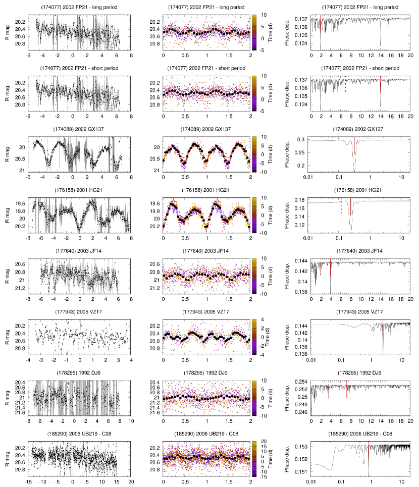
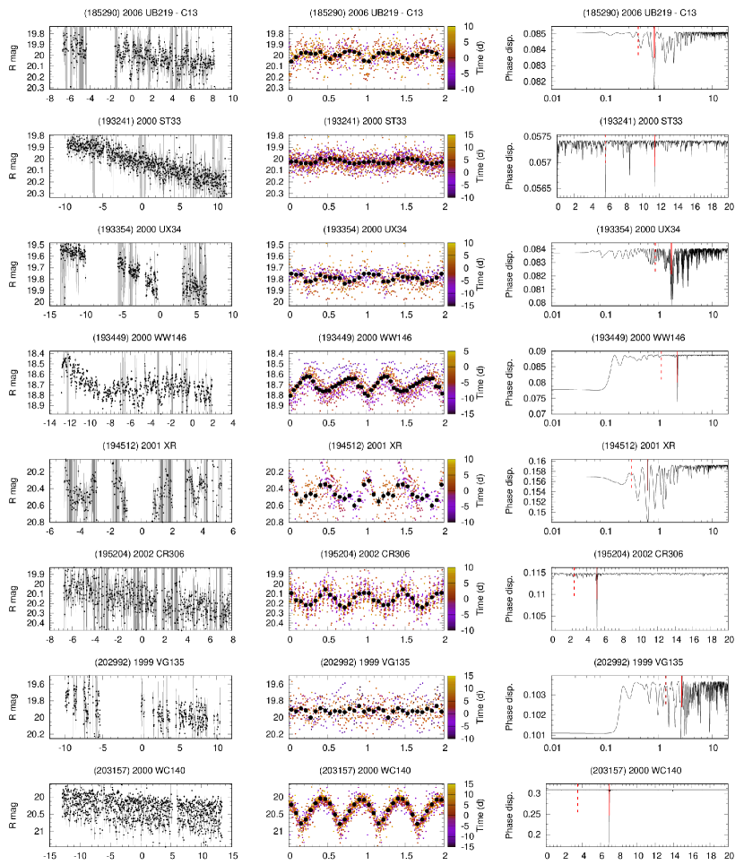
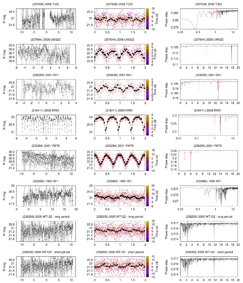
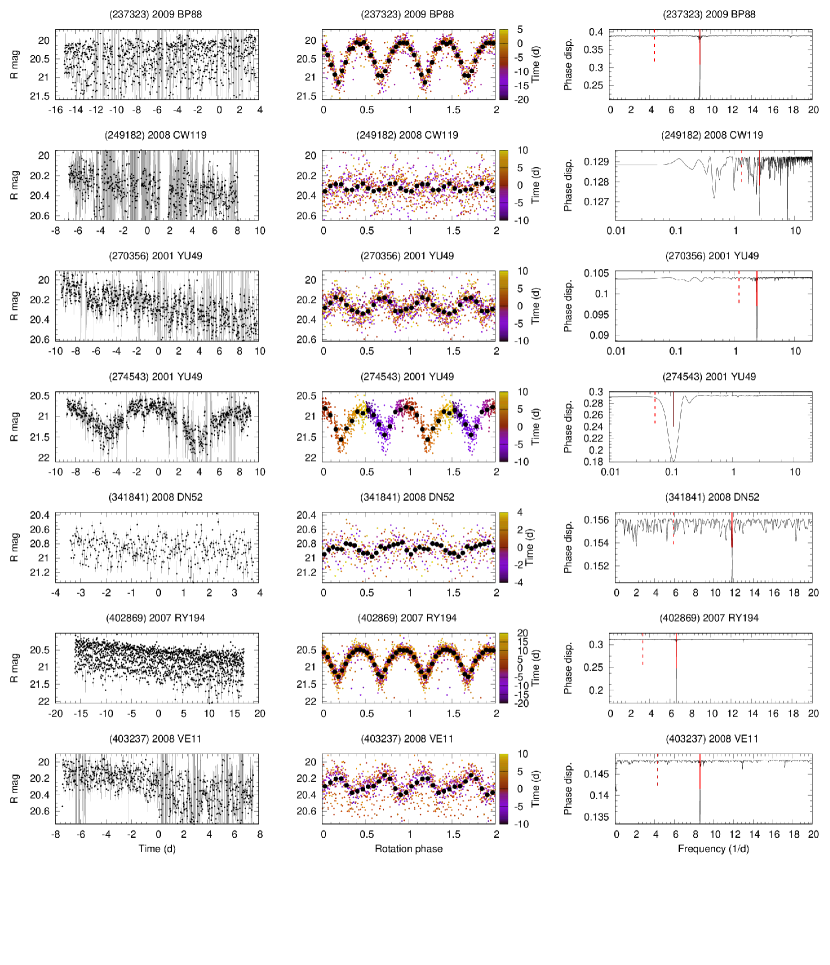
Figure 6: Light curves of Hildas observed by K2. Left: raw light curves. Middle: rectified and folded phase curves. Dots are phase-binned points, color shows time. Right: residual dispersion frequency spectra. Red solid and dashed lines mark frequencies for the single- and double-peak solutions.

Figure 6: Light curves of Hildas observed by K2. Left: raw light curves. Middle: rectified and folded phase curves. Dots are phase-binned points, color shows time. Right: residual dispersion frequency spectra. Red solid and dashed lines mark frequencies for the single- and double-peak solutions.

Figure 6: Light curves of Hildas observed by K2. Left: raw light curves. Middle: rectified and folded phase curves. Dots are phase-binned points, color shows time. Right: residual dispersion frequency spectra. Red solid and dashed lines mark frequencies for the single- and double-peak solutions.

Figure 6: Light curves of Hildas observed by K2. Left: raw light curves. Middle: rectified and folded phase curves. Dots are phase-binned points, color shows time. Right: residual dispersion frequency spectra. Red solid and dashed lines mark frequencies for the single- and double-peak solutions.

Figure 6: Light curves of Hildas observed by K2. Left: raw light curves. Middle: rectified and folded phase curves. Dots are phase-binned points, color shows time. Right: residual dispersion frequency spectra. Red solid and dashed lines mark frequencies for the single- and double-peak solutions.

Figure 6: Light curves of Hildas observed by K2. Left: raw light curves. Middle: rectified and folded phase curves. Dots are phase-binned points, color shows time. Right: residual dispersion frequency spectra. Red solid and dashed lines mark frequencies for the single- and double-peak solutions.

Figure 6: Light curves of Hildas observed by K2. Left: raw light curves. Middle: rectified and folded phase curves. Dots are phase-binned points, color shows time. Right: residual dispersion frequency spectra. Red solid and dashed lines mark frequencies for the single- and double-peak solutions.

Figure 6: Light curves of Hildas observed by K2. Left: raw light curves. Middle: rectified and folded phase curves. Dots are phase-binned points, color shows time. Right: residual dispersion frequency spectra. Red solid and dashed lines mark frequencies for the single- and double-peak solutions.

Figure 6: Light curves of Hildas observed by K2. Left: raw light curves. Middle: rectified and folded phase curves. Dots are phase-binned points, color shows time. Right: residual dispersion frequency spectra. Red solid and dashed lines mark frequencies for the single- and double-peak solutions.

Figure 6: Light curves of Hildas observed by K2. Left: raw light curves. Middle: rectified and folded phase curves. Dots are phase-binned points, color shows time. Right: residual dispersion frequency spectra. Red solid and dashed lines mark frequencies for the single- and double-peak solutions.

Figure 6: Light curves of Hildas observed by K2. Left: raw light curves. Middle: rectified and folded phase curves. Dots are phase-binned points, color shows time. Right: residual dispersion frequency spectra. Red solid and dashed lines mark frequencies for the single- and double-peak solutions.

Figure 6: Light curves of Hildas observed by K2. Left: raw light curves. Middle: rectified and folded phase curves. Dots are phase-binned points, color shows time. Right: residual dispersion frequency spectra. Red solid and dashed lines mark frequencies for the single- and double-peak solutions.

Figure 6: Light curves of Hildas observed by K2. Left: raw light curves. Middle: rectified and folded phase curves. Dots are phase-binned points, color shows time. Right: residual dispersion frequency spectra. Red solid and dashed lines mark frequencies for the single- and double-peak solutions.

References

- Alvarez-Candal (2013) Alvarez-Candal, A. 2013, A&A, 549, A34
- Brož & Vokrouhlický (2008) Brož, M., & Vokrouhlický, D. 2008, MNRAS, 390, 715
- Dahlgren et al. (1998) Dahlgren, M., Lahulla, J. F., Lagerkvist, C.-I., et al. 1998, Icarus, 133, 247
- DeMeo & Carry (2013) DeMeo, F. E., & Carry, B. 2013, AAS/Division for Planetary Sciences Meeting Abstracts #45, 45, 205.05
- De Prá et al. (2018) De Prá, M. N., Pinilla-Alonso, N., Carvano, J. M., et al. 2018, Icarus, 311, 35
- Durech et al. (2016) Durech, J., Hanus, J., Oszkiewsicz, D., et al. 2016, A&A, 587, A48
- Fraley et al. (2018) Fraley, C., et al., 2018, Package ’mclust’, version Novermber 17, 2018
- Franklin et al. (2004) Franklin, F. A., Lewis, N. K., Soper, P. R., Holman, M. J. 2004, AJ, 128, 1391