Deep Metric Structured Learning For Facial Expression Recognition

Abstract

We propose a deep metric learning model to create embedded sub–spaces with a well defined structure. A new loss function that imposes Gaussian structures on the output space is introduced to create these sub–spaces thus shaping the distribution of the data. Having a mixture of Gaussians solution space is advantageous given its simplified and well established structure. It allows fast discovering of classes within classes and the identification of mean representatives at the centroids of individual classes. We also propose a new semi–supervised method to create sub–classes. We illustrate our methods on the facial expression recognition problem and validate results on the FER+, AffectNet, Extended Cohn-Kanade (CK+), BU-3DFE, and JAFFE datasets. We experimentally demonstrate that the learned embedding can be successfully used for various applications including expression retrieval and emotion recognition.

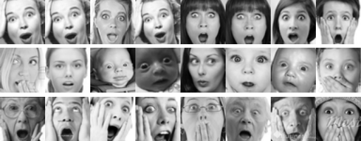
Figure 1: Classes within classes. The figure depicts some faces in the FER+ dataset classified by our method as having a surprise expression. Our method further separates these faces into other sub–classes, as shown in the three examples above. Each row contains the top eight images identified to be the closest ones to the centroid of their respective sub–class, and each represented by its own Gaussian. One could tentatively visually describe the top row as faces with strong eye and mouth expressions of surprise, the middle row with mostly mildly surprised eyes, and the bottom row faces with strong surprise expressed with wide open eyes and mouth, and hands on face. Observe the face similarities in each sub–class.

 

1 Introduction

Classical distance metrics like Euclidean distance and cosine similarity are limited and do not always perform well when computing distances between images or their parts. Recently, end–to–end methods [25, 1, 28, 31] have shown much progress in learning an intrinsic distance metric. They train a network to discriminatively learn embeddings so that similar images are close to each other and images from different classes are far away in the feature space. These methods are shown to outperform others adopting manually crafted features such as SIFT and binary descriptors [8, 27]. Feedforward networks trained by supervised learning can be seen as performing representation learning, where the last layer of the network is typically a linear classifier, e.g. a softmax regression classifier.

Representation learning is of great interest as a tool to enable semi-supervised and unsupervised learning. It is often the case that datasets are comprised of vast training data but with relatively little labeled training data. Training with supervised learning techniques on a reduced labeled subset generally results in severe overfitting. Semi-supervised learning is an alternative to resolve the overfitting problem by learning from the vast unlabeled data. Specifically, it is possible to learn good representations for the unlabeled data and use them to solve the supervised learning task.

The adoption of a particular cost function in learning methods imposes constraints on the solution space, whose shape can take any form satisfying the underlying properties induced by the loss function. For example, in the case of triplet loss [25], the optimization of the cost function leads to the creation of a solution space where every object has the nearest neighbors within the same class. Unfortunately, it does not generate a much desired probability distribution function, which is achieved by our formulation.

In theory, we would like to have the solution manifold to be a continuous function representing the true original information, because, as in the case of the facial expression recognition problem, face expressions are points in the continuous facial action space resulting from the smooth activation of facial muscles [9]. The transition from one expression to another is represented as the trajectory between the embedded vectors on the manifold surface.

The objective of this work is to offer a formulation for the creation of separable sub–spaces each with a defined structure and with a fixed data distribution. We propose a new loss function that imposes Gaussian structures in the creation of these sub-spaces. In addition, we also propose a new semi-supervised method to create sub–classes within each facial expression class, as exemplified in Figure 1.

2 Related Work

Siamese networks applied to signature verification showed the ability of neural networks to learn compact embedding [5]. OASIS [6] and local distance learning [10] learn fine-grained image similarity ranking models using hand-crafted features that are not based on deep-learning. Recent methods such as [25, 1, 28, 31] approaches the problem of learning a distance metric by discriminatively training a neural network. Features generated by those approaches are shown to outperform manually crafted features [1], such as SIFT and various binary descriptors [8, 27].

Distance Metric Learning (DML) can be broadly divided into contrastive loss based methods, triplet networks, and approaches that go beyond triplets such as quadruplets, or even batch-wise loss. Contrastive embedding is trained on paired data, and it tries to minimize the distance between pairs of examples with the same class label while penalizing examples with different class labels that are closer than a margin $\alpha$ [11]. Triplet embedding is trained on triplets of data with anchor points, a positive that belongs to the same class, and a negative that belongs to a different class [33, 14]. Triplet networks use a loss over triplets to push the anchor and positive closer, while penalizing triplets where the distance between the anchor and negative is less than the distance between the anchor and positive, plus a margin $\alpha$. Contrastive embedding has been used for learning visual similarity for products [4], while triplet networks have been used for face verification, person re-identification, patch matching, for learning similarity between images and for fine-grained visual categorization [25, 26, 31, 7, 1].

Several works are based on triplet-based loss functions for learning image representations. However, the majority of them use category label-based triplets [36, 32, 23]. Some existing works such as [6, 31] have focused on learning fine-grained representations. In addition, [36] used a similarity measure computing several existing feature representations to generate ground truth annotations for the triplets, while [31] used text image relevance, based on Google image search to annotate the triplets. Unlike those approaches, we use human raters to annotate the triplets. None of those works focus on facial expressions, only recently [30] proposed a system of facial expression recognition based on triplet loss.

3 Methodology

3.1 Structured Gaussian Manifold Loss

Let $S=\{x_{i}|x_{i}\in\mbox{$\mathbbm{R}^{D}$}\}$ be a collection of i.i.d. samples $x_{i}$ to be classified into $c$ classes, and let $w_{j}$ represent the $j$–th class, for $j=1,\ldots,c$. The computed class function $l(x)=\arg\max p(w|f_{\Theta}(x))$ returns the class $w_{j}$ of sample $x$ – maximum a posteriori probability estimate – for the neural net function $f_{\Theta}:\mbox{$\mathbbm{R}^{D}$}\to\mbox{$\mathbbm{R}^{d}$}$ drawn independently according to probability $p(x|w_{j})$ for input $x$. Suppose we separate $S$ in an embedded space such that each set $C_{j}=\{x|x\in S,l(x)=w_{j}\}$ contains the samples belonging to class $w_{j}$. Our goal is to find a Gaussian representation for each $C_{j}$ which would allow a clear separation of $S$ in a reduced space, $d\ll D$.

We assume that $p(f_{\Theta}(x)|w_{j})$ has a known parametric form, and it is therefore determined uniquely by the value of a parameter vector $\theta_{j}$. For example, we might have $p(f_{\Theta}(x)|w_{j})\sim N(\mu_{j},\Sigma_{j})$, where $\theta_{j}=(\mu_{j},\Sigma_{j})$, for $N(.,.)$ the normal distribution with mean $\mu_{j}$ and variance $\Sigma_{j}$. To show the dependence of $p(f_{\Theta}(x)|w_{j})$ on $\theta_{j}$ explicitly, we write $p(f_{\Theta}(x)|w_{j})$ as $p(f_{\Theta}(x)|w_{j},\theta_{j})$. Our problem is to use the information provided by the training samples to obtain a good transformation function $f_{\Theta}(x_{j})$ that generates embedded spaces with a known distribution associated with each category. Then the a posteriori probability $P(w_{j}|f_{\Theta}(x))$ can be computed from $p(f_{\Theta}(x)|w_{j})$ by the Bayes’ formula:

$$P(w_{j}|f_{\Theta}(x))=\frac{p(w_{j})p(f_{\Theta}(x)|w_{j},\theta_{i})}{\sum_{i}^{c}p(w_{i})p(f_{\Theta}(x)|w_{i},\theta_{i})}$$ (1)

We use the normal density function for $p(x|w_{j},\theta_{j})$. The objective is to generate embedded sub-spaces with defined structure. Thus, using the Gaussian structures:

$$p(f_{\Theta}(x)|w_{j},\mu_{j},\Sigma_{j})=\frac{1}{(2\pi)^{n/2}|\Sigma_{j}|^{1/2}}\exp(-\frac{1}{2}X^{T}\Sigma_{j}^{-1}X)$$ (2)

where $X=(f_{\Theta}(x)-\mu_{j})$. For the case $\Sigma_{j}=\sigma^{2}I$, where $I$ is the identity matrix:

$$p(x|w_{j},\mu_{j},\sigma_{j})=\frac{1}{\sqrt[]{(2\pi)^{n}}\sigma_{j}}\exp(-\frac{||f_{\Theta}(x)-\mu_{j}||^{2}}{2\sigma_{j}^{2}})$$ (3)

In a supervised problem, we know the a posteriori probability $P(w_{j}|x)$ for the input set. From this, we can define our structured loss function as the mean square error between the a posteriori probability of the input set and the a posteriori probability estimated for the embedded space:

$$\mathcal{L}_{rep}=\mathbb{E}\left\{||P(w_{j}|f_{\Theta}(x_{i}))-P(w_{j}|x_{i})||^{2}_{2}\right\}$$ (4)

We applied the steps described in Algorithm 1 to train the system. The batch size is given by $n\times c$ where $c$ is the number of classes, and $n$ is the sample size. In this work, we use $n=30$, thus for eight classes the batch size is 240, which was used for the estimation of the parameters in Equation 4.

Algorithm 1 Structured Gaussian Manifold Learning. $f_{\Theta}$: Neural Network; $S$: dataset; $C_{j}$ are the subset of the elements of class $w_{j}$; $N$: number of updates;

1:  $k\leftarrow 0$

2:  while  $k<N$  do

3:     {Sample$(x_{i},w_{i})\}\sim S$, get current batch.

4:     $z\leftarrow f_{\Theta}(x_{i}),$ representation.

5:     $\theta_{j}\leftarrow\{\mu_{j},\sigma{j}\}$ where $\sigma$ is a parameters ($\sigma=0.5$ in this work) and $\mu_{j}$ is the mean of the elements of the class $w_{j}$:

$$\mu_{j}=\frac{1}{|C_{j}|}\sum_{k\in C}z_{k}$$

where $|.|$ denotes set cardinality.

6:     Evaluation of the Loss function. For the explanation of the loss representation see equation 4:

$$\mathcal{L}\leftarrow\mathcal{L}_{rep}(z_{i},w_{i},\mu,\sigma)+\frac{1}{|\Omega|}\sum_{k}||f_{\Theta}(x_{k})||_{2}$$

where $x_{k}\in\Omega$

7:     $\Theta^{t+1}=\Theta^{t}-\nabla\mathcal{L}$, backward and optimization steps.

8:  end while

We define the accuracy of the model as the ability of the parameter vector $\theta$ to represent the test dataset in the embedded space.

3.2 Deep Gaussian Mixture Sub-space

The same facial expression may possess a different set of global features. For example, ethnicity can determine specific color and shape, while age provides physiological differences of facial characteristics; moreover, gender, weight, and other features can determine different facial characteristics, while having the same expression. Our proposal can group and extract these characteristics automatically. We propose to represent each facial expression class as a Gaussians Mixture. These Gaussian parameters are obtained in an unsupervised way as part of the learning processes. We start from a representation space given by Algorithm 1. Subsequently, a clustering algorithm is applied to separate each class into a new class subset. This process is repeated until reaching the desired granularity level. Algorithm 2 shows the set of steps to obtain the new sub-classes.

Algorithm 2 Deep Gaussian Mixture Sub-space Learning. $L$: Maximum level of subdivisions for the class; $f_{\Theta}$: Neural Network; $StructureGaussianManifold$: Structure Gaussian Manifold Algorithm 1; $EM$: Expectation Maximization Algorithm; $S$: dataset; $C_{j}$ are the subset of the elements of class $w_{j}$; $N$: number of updates;

1:  $l\leftarrow 1$

2:  $X,Y\sim S$

3:  $\hat{Y}\leftarrow Y$

4:  while  $l<L$  do

5:     $\Theta\leftarrow$StructureGaussianManifold$(\{X,\hat{Y}\},N)$

6:     $Z=f_{\Theta}(X)$

7:     $\hat{Y}\leftarrow\{\oslash\}$

8:     $k\leftarrow 0$

9:     for all  class $w_{j}$  do

10:        $Z_{c}=\{z~{}|~{}\forall z\in C_{j}\}$

11:        $g\leftarrow EM(l,Z_{c})$

12:        $\hat{Y}=\{\hat{Y},g+k\}$

13:        $k+=l$

14:     end for

15:  end while

4 Experiments

4.1 Protocol

For the evaluation of the clustering task, we use the F1-measure and Normalized Mutual Information (NMI) measures. The F1-measure computes the harmonic mean of the precision and recall, $F1=\frac{2PR}{P+R}$. The NMI measure take as input a set of clusters $\Omega=\{o_{1},\ldots,o_{k}\}$ and a set of ground truth classes $\mathcal{G}=\{g_{1},\ldots,g_{k}\}$, $o_{i}$ indicates the set of examples with cluster assignment $i$ and $g_{j}$ indicates the set of examples with the ground truth class label $j$. Normalized mutual information is defined by the ratio of mutual information and the average entropy of the clusters and the entropy of the labels, $NMI(\Omega,\mathcal{G})=\frac{I(\Omega;\mathcal{G})}{2(H(\Omega)+H(\mathcal{G}))}$, for complete details see [21]. For the retrieval task, we use the Recall@K [15] measure. Each test image (query) first retrieves K Nearest Neighbour (KNN) from the test set and receives score $1$ if an image of the same class is retrieved among the KNN, and $0$ otherwise. Recall@K averages those score over all the images. Moreover, we also evaluate accuracy, i.e. the fraction of results that are the same class as queried image, averaged over all queries. While the classification task is evaluated using KNN.

For the training process, we use the Adam method [16] with a learning rate of 0.0001 and batch size of 256 (samples of size 32 to estimate the parameters in each iteration). In the TripletLoss case, we used 128 triplets in each batch. The neural networks were initialized with the same weights in all cases.

4.2 Result

4.2.1 Representation and Recover

The groups used for the evaluation of the measures are obtained using $K$-means, whereas $K$ equals the number of classes (8 in the case of the FER+ [2], AffectNet [24], CK+ [19] datasets, and 7 for JAFFE [20] and BU-3DFE [34] datasets).

The results obtained for the clustering task show that the proposed method presents good group quality (see table 1) in similar domains. As can be observed, the results are degraded for different domains. In general, we observe that the TripletLoss is most robust to the change of domains on all models. However, the best result is achieved using the proposed method for the RestNet18 [12] model in FER+, CK+, and BU-3DFE.

Method	Arch.	FER+†	AffectNet‡	JAFFE	CK+	BU-3DFE
TripletLoss	FMPNet[35]	55.257	10.627	19.528	71.129	34.901
	CVGG13[3]	67.384	9.103	28.295	68.303	27.275
	AlexNet[17]	67.035	12.945	30.241	68.800	27.039
	ResNet18[12]	64.457	15.588	31.046	74.028	36.708
	PreActResNet18[13]	57.904	8.452	20.699	70.079	27.580
SGMLoss	FMPNet[35]	57.880	10.469	26.196	77.839	36.559
	CVGG13[3]	65.139	10.355	24.293	66.062	27.233
	AlexNet[17]	62.091	10.582	24.560	65.230	28.115
	ResNet18[12]	68.840	12.333	30.382	77.902	37.545
	PreActResNet18[13]	51.425	6.886	23.216	61.413	26.104

Table 1: The NMI (%) of the clustering task for all datasets applying the TripletLoss and SGMLoss models trained on FER+. SGMLoss: Structured Gaussian Manifold Loss, Arch: Architecture, FER+^†: FER+ test dataset, AffectNet^‡: validation dataset. JAFFE CK+ and BU3DFE datasets are used as test set.

 

Figure 2 shows a 2D t-SNE [29] visualization of the learned SGMLoss embedding space using the FER+ training set. The amount of overlap between the two categories in this figure roughly demonstrates the extent of the visual similarity between them. For example, happy and neutral have some objects overlap, indicating that these cases could be confused easily, and both of them have a very low overlap with fear indicating that they are visually very distinct from fear. Also, the spread of a category in this figure indicates the visual diversity within that category. For example, happiness category maps to some distinct regions indicating that there are some visually distinct modes within this category.

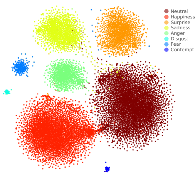
Figure 2: Barnes-Hut t-SNE visualization [29] of the SGMLoss for the FER+ database. Each color represents one of the eight emotions including neutral.

 

Figure 3 shows the results obtained in the recovery task (Recall@K and Acc@K measures) for $K=\{1,2,4,8,16,32\}$. TripletLoss obtains better recovery results for all K but to the detriment of accuracy. Our method manages to increase its recovery value while preserving quality. It means that most neighbors are of the same class. Figure 4 shows the top-5 retrieved images for some of the queries on CelebA dataset [18]. The overall results of the proposed SGMLoss embedding are clearly better than the results of TripletLoss embedding.

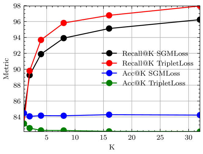
Figure 3: Recall@K and Acc@K measures for the test split FER+ dataset. The applied model was the ResNet18 having $K=\{1,2,4,8,16,32\}$.

 

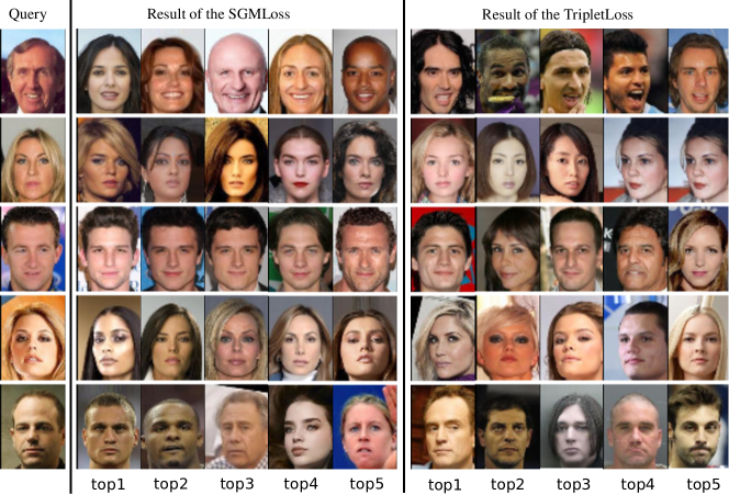
Figure 4: Top-5 images retrieved using SGMLoss (left) and TripletLoss (right) embeddings. The overall results of the SGMLoss match the query set apparently better when compared to TripletLoss.

 

4.2.2 Classification

The proposed SGMLoss method can be used for FER by combining it with the KNN classifier. Figure 5 shows the average F1-score of the SGMLoss and TripletLoss on the FER+ validation set as a function of the number of neighbors used. F1-score is maximized for K=11.

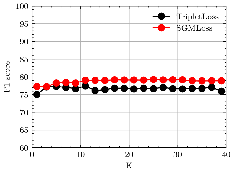
Figure 5: Classification performance of the SGMLoss and TripletLoss on the FER+ validation set when combined with KNN classifier.

 

Table 2 compares the classification performance of the SGMLoss embedding (using 11 neighbors) with TripletLoss and CNN models. In general, our method obtains the best classification results for all architectures. ResNet18 CNN model does not obtains a significant higher accuracy. Moreover, our results surpass the accuracy 84.99 presented in [2].

Method	Arch.	Acc.	Prec.	Rec.	F1
CNN	FMPNet[35]	79.535	66.697	68.582	67.627
	CVGG13[3]	84.316	75.151	67.425	71.079
	AlexNet[17]	86.038	77.658	68.657	72.881
	ResNet18[12]	87.695	85.956	69.659	76.954
	PreActResNet18[13]	82.372	76.915	65.238	70.597
TripletLoss	FMPNet[35]	82.563	79.554	62.406	69.944
	CVGG13[3]	85.974	82.034	68.112	74.428
	AlexNet[17]	86.038	80.598	67.895	73.703
	ResNet18[12]	87.121	78.543	68.378	73.109
	PreActResNet18[13]	83.519	74.081	64.856	69.162
SGMLoss	FMPNet[35]	83.360	78.806	66.520	72.143
	CVGG13[3]	86.261	86.321	67.341	75.659
	AlexNet[17]	86.643	86.182	67.673	75.814
	ResNet18[12]	87.631	88.614	68.724	77.412
	PreActResNet18[13]	84.316	89.008	66.519	76.138

Table 2: Classification results of the CNN, TripletLoss and SGMLoss models trained on FER+. SGMLoss: Structured Gaussian Manifold Loss, Arch: Architecture, FER+^†: FER+ test dataset, AffectNet^‡ validation dataset.

 

The Facial Expression dataset constitute a great challenge due to the subjectivity of the emotions [22]. The labeling process requires the effort of a group of specialists to make the annotations. FER+ and AffectNet datasets contains many problems in the labels. In [2] an effort was made to improve the quality of the labels of the FER+ (dataset used in our experiments) by re-tagging the dataset using crowd sourcing. Figure 6 shows some mislabeled images retrieved by our method. The scale, position, and context could influence the decision of a non-expert tagger such as those in crowd sourcing.

Experimental results show the quality of the embedded representation obtained by SGMLoss in the classification problems. Our representation improves the representation obtained by TripletLoss, which is the method most used in the identification and representation problems.

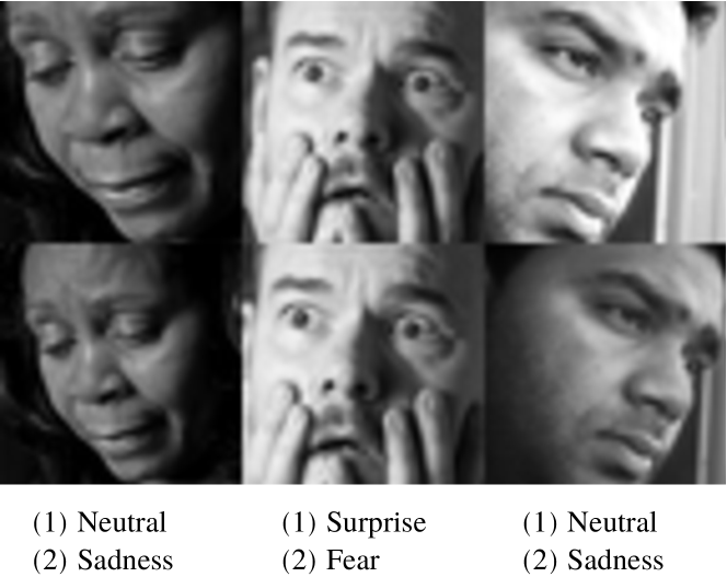
Figure 6: Examples of mislabeled images on the FER+ dataset that were recovery using SGMLoss. The first row show the result of the query (1) and the second row the result (2). We can clearly observer that two very similar images have different labels in the dataset.

 

4.2.3 Clustering

For the training process, we use the Adam method [16] with a learning rate of 0.0001, a batch size of 640 and 500 epoch. The maximum level of subdivision used is L=5 (this value guarantee that the batch for a subclass in this level to be 128). The ResNet18 architecture is selected to train the FER+ dataset. The objective of this experiment is to visually analyse the clustering obtained by this approach.

The results shown in Figure 7 present 64-dimensional embedded space using the Barnes-Hut t-SNE visualization scheme [29] using the Deep Gaussian Mixture Sub-space model for the FER+ dataset. The method created five Gaussian sub-spaces for the unsupervised case for each class.

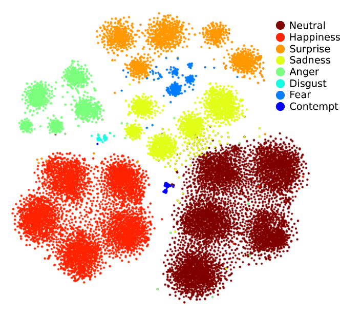
Figure 7: Barnes-Hut t-SNE visualization [29] of the Deep Gaussian Mixture Sub-space for the FER+ database. Each color represents one of the eight emotions including neutral.

 

For the clustering task, all embedded vectors are calculated and EM method is applied creating 40 groups. For each group, the medoid is calculated. The medoid is the object in the group closest to the centroid (mean to the sample). The Top-k of a group contains the k-objects nearer to the medoid of the group.

Figure 8 shows the Top-16 images obtained for the happiness category. The first group (Figure 8 (a) ) shows an expression of happiness closer to surprise (raised eyebrows and open mouth) with the shape of the eyes similar to each other. The second group (Figure 8 (b)) represents an expression closer to contempt. The third group (Figure 8 (c)) shows an expression of more intense happiness (the teeth are shown in all cases) with the shape of the mouth very similar to each other. In the fourth case (Figure 8 (d) ) shows a subcategory that is present in all facial expressions. Babies are a typically expected subset due to the intensity of expression and the physiognomical formation. Generally babies and children from 1 to 4 years old present facial expressions of greater intensity. The last group (Figure 8 (f) ) represents people with glasses and large eyes.

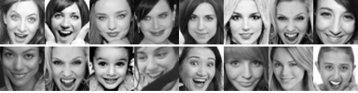
(a)

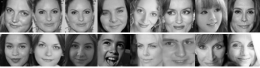
(b)

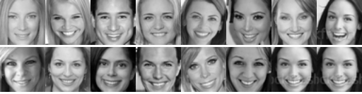
(c)

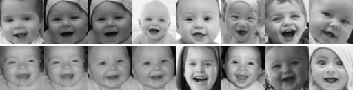
(d)

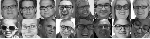
(f)

Figure 8: Top-16 images of the clustering obtained from the class happiness on the FER+ dataset.

 

The presented method is a powerful tool for tasks such as photo album summarization. In this task, we are interested in summarizing the diverse expression content present in a given photo album using a fixed number of images. Figure 9 shows 5 of the 40 groups obtained on AffectNet dataset. The obtained groups show great similarity in terms of FER. These results demonstrate the generalization capacity of the proposed method and its applicability to problems of FER clustering.

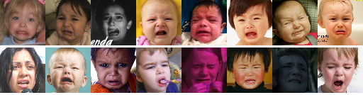
(a)

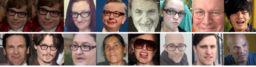
(b)

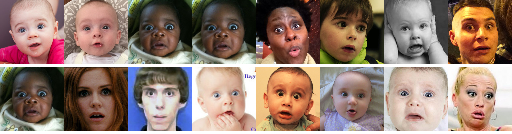
(c)

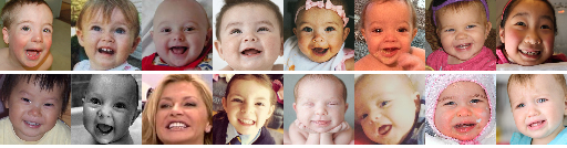
(d)

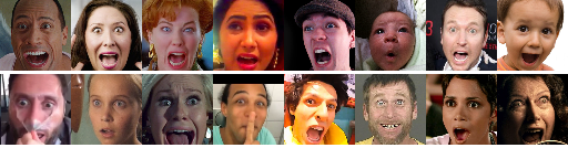
(f)

Figure 9: Top-16 images of the 5 clustering obtained from the AffectNet dataset.

 

5 Conclusions

We introduced two new metric learning representation models in this work, namely Deep Gaussian Mixture Subspace Learning and Structured Gaussian Manifold Learning. In the first model, we build a Gaussian representation of expressions leading to a robust classification and grouping of facial expressions. We illustrate through many examples, the high quality of the vectors obtained in recovery tasks, thus demonstrating the effectiveness of the proposed representation. In the second case, we provide a semi-supervised method for grouping facial expressions. We were able to obtain embedded subgroups sharing the same facial expression group. These subgroups emerged due to shared specific characteristics other than the general appearance. For example, individuals with glasses expressing a happy appearance.

References

- [1] Vassileios Balntas, Edgar Riba, Daniel Ponsa, and Krystian Mikolajczyk. Learning local feature descriptors with triplets and shallow convolutional neural networks. In BMVC, volume 1, page 3, 2016.
- [2] Emad Barsoum, Cha Zhang, Cristian Canton Ferrer, and Zhengyou Zhang. Training deep networks for facial expression recognition with crowd-sourced label distribution. In ACM International Conference on Multimodal Interaction (ICMI), 2016.
- [3] Emad Barsoum, Cha Zhang, Cristian Canton Ferrer, and Zhengyou Zhang. Training deep networks for facial expression recognition with crowd-sourced label distribution. In ACM International Conference on Multimodal Interaction (ICMI), 2016.
- [4] Sean Bell and Kavita Bala. Learning visual similarity for product design with convolutional neural networks. ACM Transactions on Graphics (TOG), 34(4):98, 2015.
- [5] Jane Bromley, Isabelle Guyon, Yann LeCun, Eduard Säckinger, and Roopak Shah. Signature verification using a” siamese” time delay neural network. In Advances in Neural Information Processing Systems, pages 737–744, 1994.
- [6] Gal Chechik, Varun Sharma, Uri Shalit, and Samy Bengio. Large scale online learning of image similarity through ranking. Journal of Machine Learning Research, 11(Mar):1109–1135, 2010.
- [7] Yin Cui, Feng Zhou, Yuanqing Lin, and Serge Belongie. Fine-grained categorization and dataset bootstrapping using deep metric learning with humans in the loop. In Proceedings of the IEEE Conference on Computer Vision and Pattern Recognition, pages 1153–1162, 2016.
- [8] Alexey Dosovitskiy, Philipp Fischer, Jost Tobias Springenberg, Martin Riedmiller, and Thomas Brox. Discriminative unsupervised feature learning with exemplar convolutional neural networks. IEEE transactions on pattern analysis and machine intelligence, 38(9):1734–1747, 2016.
- [9] Paul Ekman, Wallace V Friesen, and Joseph C Hager. Facial action coding system. A Human Face, 2002.
- [10] Andrea Frome, Yoram Singer, and Jitendra Malik. Image retrieval and classification using local distance functions. In Advances in neural information processing systems, pages 417–424, 2007.
- [11] Raia Hadsell, Sumit Chopra, and Yann LeCun. Dimensionality reduction by learning an invariant mapping. In Computer vision and pattern recognition, 2006 IEEE computer society conference on, volume 2, pages 1735–1742. IEEE, 2006.
- [12] Kaiming He, Xiangyu Zhang, Shaoqing Ren, and Jian Sun. Deep residual learning for image recognition. CoRR, abs/1512.03385, 2015.
- [13] Kaiming He, Xiangyu Zhang, Shaoqing Ren, and Jian Sun. Identity mappings in deep residual networks. In European conference on computer vision, pages 630–645. Springer, 2016.
- [14] Elad Hoffer and Nir Ailon. Deep metric learning using triplet network. In International Workshop on Similarity-Based Pattern Recognition, pages 84–92. Springer, 2015.
- [15] Herve Jegou, Matthijs Douze, and Cordelia Schmid. Product quantization for nearest neighbor search. IEEE transactions on pattern analysis and machine intelligence, 33(1):117–128, 2011.
- [16] Diederik P. Kingma and Jimmy Ba. Adam: A method for stochastic optimization. CoRR, abs/1412.6980, 2014.
- [17] Alex Krizhevsky. One weird trick for parallelizing convolutional neural networks. CoRR, abs/1404.5997, 2014.
- [18] Ziwei Liu, Ping Luo, Xiaogang Wang, and Xiaoou Tang. Deep learning face attributes in the wild. In Proceedings of the IEEE international conference on computer vision, pages 3730–3738, 2015.
- [19] Patrick Lucey, Jeffrey F Cohn, Takeo Kanade, Jason Saragih, Zara Ambadar, and Iain Matthews. The Extended Cohn-Kanade Dataset (CK+): A complete dataset for action unit and emotion-specified expression. In Computer Vision and Pattern Recognition Workshops (CVPRW), 2010 IEEE Computer Society Conference on, pages 94–101. IEEE, 2010.
- [20] Michael Lyons, Shigeru Akamatsu, Miyuki Kamachi, and Jiro Gyoba. Coding facial expressions with gabor wavelets. In Automatic Face and Gesture Recognition, 1998. Proceedings. Third IEEE International Conference on, pages 200–205. IEEE, 1998.
- [21] Christopher D Manning, Prabhakar Raghavan, Hinrich Schütze, et al. Introduction to information retrieval, volume 1. Cambridge university press Cambridge, 2008.
- [22] Pedro Marrero-Fernández, Arquímedes Montoya-Padrón, Antoni Jaume-I-Capó, and Jose Maria Buades Rubio. Evaluating the research in automatic emotion recognition. IETE Technical Review (Institution of Electronics and Telecommunication Engineers, India), 31(3):220–232, 2014.
- [23] Hyun Oh Song, Yu Xiang, Stefanie Jegelka, and Silvio Savarese. Deep metric learning via lifted structured feature embedding. In Proceedings of the IEEE Conference on Computer Vision and Pattern Recognition, pages 4004–4012, 2016.
- [24] R.W. Picard. Affective Computing. MIT Press, 2000.
- [25] Florian Schroff, Dmitry Kalenichenko, and James Philbin. Facenet: A unified embedding for face recognition and clustering. In Proceedings of the IEEE conference on computer vision and pattern recognition, pages 815–823, 2015.
- [26] Hailin Shi, Yang Yang, Xiangyu Zhu, Shengcai Liao, Zhen Lei, Weishi Zheng, and Stan Z Li. Embedding deep metric for person re-identification: A study against large variations. In European Conference on Computer Vision, pages 732–748. Springer, 2016.
- [27] Edgar Simo-Serra, Eduard Trulls, Luis Ferraz, Iasonas Kokkinos, Pascal Fua, and Francesc Moreno-Noguer. Discriminative learning of deep convolutional feature point descriptors. In Computer Vision (ICCV), 2015 IEEE International Conference on, pages 118–126. IEEE, 2015.
- [28] Hyun Oh Song, Yu Xiang, Stefanie Jegelka, and Silvio Savarese. Deep metric learning via lifted structured feature embedding. In Computer Vision and Pattern Recognition (CVPR), 2016 IEEE Conference on, pages 4004–4012. IEEE, 2016.
- [29] Laurens Van Der Maaten. Accelerating t-sne using tree-based algorithms. Journal of machine learning research, 15(1):3221–3245, 2014.
- [30] Raviteja Vemulapalli and Aseem Agarwala. A compact embedding for facial expression similarity. In Proceedings of the IEEE Conference on Computer Vision and Pattern Recognition, pages 5683–5692, 2019.
- [31] Jiang Wang, Thomas Leung, Chuck Rosenberg, Jinbin Wang, James Philbin, Bo Chen, Ying Wu, et al. Learning fine-grained image similarity with deep ranking. arXiv preprint arXiv:1404.4661, 2014.
- [32] Jian Wang, Feng Zhou, Shilei Wen, Xiao Liu, and Yuanqing Lin. Deep metric learning with angular loss. In Proceedings of the IEEE International Conference on Computer Vision, pages 2593–2601, 2017.
- [33] Kilian Q Weinberger and Lawrence K Saul. Distance metric learning for large margin nearest neighbor classification. Journal of Machine Learning Research, 10(Feb):207–244, 2009.
- [34] Lijun Yin, Xiaozhou Wei, Yi Sun, Jun Wang, and Matthew J Rosato. A 3D facial expression database for facial behavior research. In Automatic face and gesture recognition, 2006. FGR 2006. 7th international conference on, pages 211–216. IEEE, 2006.
- [35] Zhiding Yu and Cha Zhang. Image based static facial expression recognition with multiple deep network learning. In Proceedings of the 2015 ACM on International Conference on Multimodal Interaction, ICMI ’15, pages 435–442, New York, NY, USA, 2015. ACM.
- [36] Bohan Zhuang, Guosheng Lin, Chunhua Shen, and Ian Reid. Fast training of triplet-based deep binary embedding networks. In Proceedings of the IEEE Conference on Computer Vision and Pattern Recognition, pages 5955–5964, 2016.