Corroborating pseudoscalar probing model with pulsar polarisation datasets

Abstract.

Recently, we have used, pulsar polarisation datasets, on circular polarisation degree [1] & linear polarisation position angle [2], to relate with well established theories, on ellipticity parameter and linear polarisation position angles, accrued by unpolarised photons, while undergoing photon-ALP oscillations, inside a magnetised medium. This has given us parameter values such as ALP mass and its coupling to photons [3]. To further test this, we now switch to different wavebands, other than earlier 21 cm wavelength, and check for the validity of our model. Here we use two data sets [4] on circular polarisation degree of identical pulsars observed in two different wavebands. We show, correlation between these two new sets of data and our model using the composite product variable of ALP mass and its coupling to photons, exist. We also check whether our model hypothesis that one physical effect, namely ALP-photon mixing is sufficient to, estimate ALP parameters, faithfully, or not. We conclude by describing other pertinent physical effects that may be included into our model to explain the circular polarisation degree of pulsars,independent of its operating wavelength of observation.

1. Introduction

Generic pseudoscalars [5, 6, 7, 8, 9, 10] or Axion-like particles (ALPs) are well motivated by many throeries beyond standard model of particle physics [11, 12]. The proposed interconversion of photon to ALPs mediated by a background magnetic field has been explored for more than two[13, 14, 15, 16] decades to extract the mass & couling strength to photons, of ALPs. This field has been traversed by both phenomenologically [17, 18, 19, 20, 21, 22, 23, 24, 25, 26, 27, 28, 29, 30, 31, 32] and observationally [33, 34, 35, 36, 37, 38, 39, 40]. Here we shall turn our attention to the polarisation properties of highly degenerate compact stars [41, 42, 43], commmonly referred to as neutron star. We have recently shown that experimental observation of ellipticity parameters of such objects [44, 45, 46, 47] may also be related to a theoretical ellipticity parameter which assumes a suitable $\gamma$-ALP interconversion model, with the help of correlation and regression we obtained the ALP mass & its coupling to photons, in an earlier work [3]. The composite product of these two pseudoscalar parameters, may now be harnessed in reverse, to estimate waveband frequencies in which the polarisation observations are made. In so doing, we utilise another dataset describing polarisation details of pulsars in two different wavebands, to calculate the observational ellipticity parameter. Putting the composite product pseudoscalar parameters and magnetic field, into the theoretical ellipticity parameter, leaves only one unknown quantity, i.e. the frequency of observations, aside. If our hypothesis is correct about this model of ALP-$\gamma$ mixing, then the slope of regression between theoretical and experimental ellipticity will fit the value of the frequency of of observation, in both the cases. Matches of frequencies shall increase the confidence in our simple model. Otherwise possible improvements may be implemented over it.

2. Data & Model

The following data shown in table no. (3) is obtained from the reference no. [4]. It contains the spin down luminosity ${\rm E}$, pulsar spin period ${\rm P}$ and spin period time derivative ${\rm\dot{P}}$, for one hundred pulsars observed in two frequencies, 333 MHz & 618 MHz. Out of which 86 of them have complete polarisation information, that are used here. However a fraction of the data is only given here, for want of space. Following the basic pulsar model [42] we may derive pulsar magnetic field $\mathfrak{B}$.

(1) $$\mathfrak{B=10^{12}}{\rm\left(\dot{P}\right)_{-15}^{\frac{1}{2}}\left(P\right)_{sec}^{\frac{1}{2}}Gauss}$$

The ellipticity parameter can then be evaluated by the following formula [3, 48, 49]

(2) $$\chi={\rm\frac{1}{96\omega}\left(g_{\phi\gamma\gamma}\mathfrak{B}m_{\phi}\right)^{2}z^{3}}$$

Given that the distance ${\rm z}$ is fixed to 10 kilometres & the magnetic field $\mathfrak{B}$ is calculated from the data, we can calculate a theoretical estimate of the ellipticity parameter. In so doing we use the values of pseudoscalar ALP parameters derived in [3], provided we use employ the ALP parameters as derived therein, and the frequency used in [4]. However, this also entails an unique opportunity to pit the the experimental ellipticity parameter, as given by

(3) $$\chi=\frac{1}{2}\arctan\frac{|\mathbb{V}|}{{\rm\mathbb{P}_{lin}}}$$

with that of the theoretical one (2), modulo the value of the observational frequency, in what is known as a regression analysis. The interceptless slope or the regression coefficient shall then reveal to us the frequency used for the experiment. A close match shall boost our confidence in our model. However, we shall look for other statistical checks and balances such that how our results are self consistent (closely correlated), and whether or not, the result thus obtained is due to serendipitous stroke of luck, such as providential positioning of outliers in the data. We shall repeat this method to chek our model for both the wavebands of observation as given in our data source reference [4]. The goodness of fit for both the cases shall also inspected. Also, possible reasons for the differences shall be attributed to effects that are already known in [50].

3. Result of Regression Analysis

The result of the statistical analysis for the waveband 333 MHz is given in table no. (1)

Coefficients	Mean	Std. Error	F-Statistics	t-value	Pr$\,\left(>|t|\right)$
Slope	2.050e-16	6.627e-17	9.5686	3.093	0.00268 $\ast\ast$

Table 1. Result for 333MHz

This is quite good fit with two stars at $4\sigma$ level. The above result translates into a frequency of ${\rm 311.446\pm 100.68\,MHz}$. Except for the large WSSR error, the fit is quite convincing.

The summary graph containing the prediction limits and confidence intervals (95%) of the fit is given in fig. no. (1)

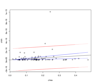
Figure 1. Summary fit graph for 333 MHz with confidence interval in blue and prediction interval in red.

Next, we look for other fitting characteristics for this waveband, before going onto the other waveband. These include (standardized) residues plot, Q-Q plot & cook’s distance plot, given in fig. no. (2), so that we know the fit is not accidental due to fortuitous placements of outliers. We also note the normal nature of the distribution of the data points from Q-Q plot.

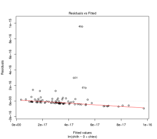
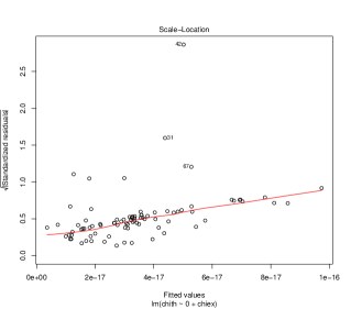
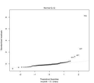
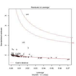
Figure 2. The fit characteristic curves for 333 MHz

Now result of the statistical analysis for the waveband 618 MHz is given in table no. (2)

Coefficients	Mean	Std. Error	F-Statistics	t-value	Pr$\,\left(>|t|\right)$
Slope	1.763e-16	6.692e-17	6.9422	2.635	0.01$\ast$

Table 2. Result for 618MHz

As compared to the earlier wavebands case, this is a poor fit, with single star and at $3\sigma$ level. This result translates into $267.843\pm 101.67{\rm MHz}$. This, even with the large associated WSSR errorbars fails, quite markedly, to reproduce the observational frequency. We shall discuss briefly, the reasons behind this, in the next section.

The summary graph containing the prediction limits and confidence intervals (95%) of the fit, for this waveband, too, is given in fig. no. (3)

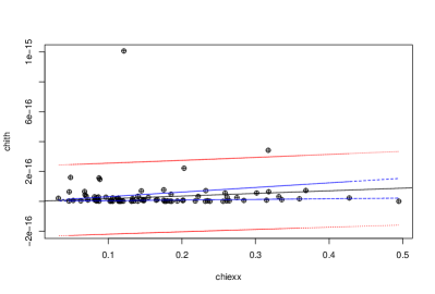
Figure 3. Summary fit graph for 618 MHz with confidence interval in blue and prediction interval in red.

Next, for the sake of completeness, we look for other fitting characteristics for this waveband, too. These include, once again, (standardized) residues plot, Q-Q plot & cook’s distance plot, given in fig. no. (4), so that we know the fit is not accidental due to fortuitous placements of outliers. We also note the normal nature of the distribution of the data points from Q-Q plot.

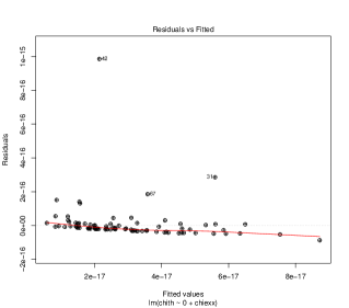
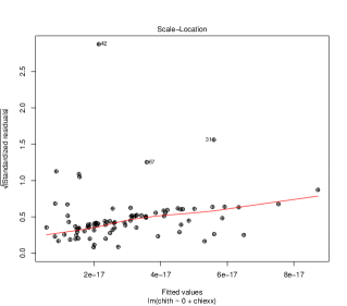
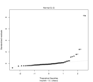
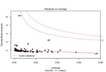
Figure 4. The fit characteristic curves for 618 MHz

4. Discussion

we have been successful in at least reproducing one observational radio frequency, successfully, employing previously calculated values of ALPs parameters. Also, the estimate veered off course for the other observational frequency. The reason for this discrepancy requires deeper investigation, whereupon we shall only underscore some tell tale signature. We note that 618 MHz roughly translates to $4.067\times 10^{-7}{\rm eV}.$ In case the limitting frequency as given in [50] evaluates to this value, near the pulsar polar cap surroundings, as shown in fig. no. (5) then we may have to take into account the Faraday effect, along side the mixing effect. Then we have to redo all our calculation done previously in [3] to accomodate for borderline frequencies. The limmiting frquency is given by:

(4) $${\rm\omega_{L}=\left|\frac{\omega_{B}\omega_{P}\left(\omega_{p}^{2}-m_{\phi}^{2}\right)}{g_{\phi\gamma\gamma}^{2}\mathfrak{B}^{2}}\right|}^{\frac{1}{3}}$$

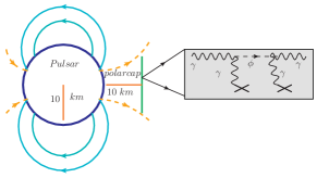
Figure 5. ALPs-$\gamma$ interconversion in the polar cap region

Assuming, the secondary plasma frequency as given by [51] we can actually compute this value quite accurately. The limitting frequency indeed ${\rm\omega_{L}}$evaluates to $\sim{\rm 10^{-7\,}eV}$. There are also other geometrical effects that may be important here. As per the emission height to frequency mapping of pulsar radiation [52], high frequency radio beams are generated parallel to the magnetic axis [53] whereas low frequency beams are generated perpendicularly. Hence it is the intermediate frequency radio beam that will more prone to exhibit Faraday type mixing between two photon polarisations. It is also a known fact, that, Faraday effect is also more pronounced at intermediate regions of frequency as given in by the stokes parameter in ref. [50], vide fig. no. 1 & 2 therein.

5. Conclusion & Outlook

The present analysis has proven to be insightful. On one hand it boosts our confidence in the simple model that leads us to the ALPs parameters. It also points to us the shortcoming of this simple model that may creep up in borderline cases, on the other hand. We shall carefully study and incorporate these effects and shall aspire to plug the theoretical gaps in the ALPs parameter extraction model.

	333MHz		618 Mhz						Unitless
Jname	%L	%IVI	%L	%IVI	Period(s)	${\rm\dot{P}}$ -15(ss-1)	$\mathfrak{B}$ (GeV2)	$\chi_{th}$(GeV)	$\chi_{Ex@333\,Hz}$	$\chi_{Ex@6218\,Hz}$
J0034-0721	19.7	15.9	20.4	7.7	0.942	0.408	2.7405656827334E-08	2.84620291587993E-18	0.339529618702371	0.180458870791069
J0134-2937	70.7	11	69.5	16.6	0.136	0.0784	4.56469923870566E-09	7.89604772133709E-20	0.077174732446713	0.117228154393456
J0151-0635	33.9	11	38.9	11.9	1.464	0.4436	3.56246814269074E-08	4.80936133524069E-18	0.15688246056648	0.148436164504233
J0152-1637	15.5	12.7	14.4	10.5	0.832	1.3	4.59746065840699E-08	8.009796307959E-18	0.34321587899093	0.315016954772958
J0304+1932	39.5	12	37.6	11.2	1.387	1.3	5.93600952236433E-08	1.3352869566273E-17	0.147468529424404	0.144751835980694
J0452-1759	24.3	4.5	15.8	3.4	0.548	5.75	7.84709452064903E-08	2.33347523727615E-17	0.091555408631242	0.10597881862131
J0525+1115	23.1	9.6	25.8	14.5	0.354	0.0736	7.13551330788753E-09	1.92946040057403E-19	0.196934305368181	0.256010669791881
J0543+2329	74.7	5.3	61.7	12.1	0.245	15.4	8.58673548957926E-08	2.79409776903932E-17	0.03541588634456	0.096826297710216
J0614+2229	74.9	13.3	68.7	12.3	0.334	59.4	1.96902458246107E-07	1.46922295517181E-16	0.087869148342684	0.088581116851283
J0629+2415	29.9	14.7	30.9	11.3	0.476	2	4.31323535550751E-08	7.05004260833669E-18	0.228468150184742	0.175294355633881
J0630-2834	27.7	5.1	55.7	7.6	1.244	7.12	1.31563333598872E-07	6.5592648523076E-17	0.091038212022324	0.067803914675729
J0659+1414	78.1	9.7	69.6	12.3	0.384	55	2.03156928978561E-07	1.56404306605116E-16	0.06178348632263	0.087459040244205
J0729-1836	25.8	10	29.7	14.9	0.51	19	1.37608915060035E-07	7.1759362263427E-17	0.184884267396709	0.232496751604164
J0738-4042	11.9	4.3	13.2	6.7	0.374	1.62	3.44094705772699E-08	4.48684854573428E-18	0.173372674007781	0.234844915770753
J0742-2822	71.2	2.5	90	5.8	0.166	16.8	7.38232850940677E-08	2.06524777585392E-17	0.017548970232895	0.032177725823632
J0758-1528	22.7	7	17.8	4.1	0.682	1.62	4.64659025065047E-08	8.18190028928016E-18	0.149558967455819	0.113194253747117
J0837+0610	12.8	4.1	8.4	6.2	1.273	6.8	1.30062872220477E-07	6.41050302886615E-17	0.154993195623442	0.317919211761873
J0905-5127	81.7	9.2	81.8	7.7	0.346	24.9	1.29754493042206E-07	6.38014045040587E-17	0.056067360888871	0.04692773430486
J0908-1739	23.5	5.1	20.6	5.7	0.401	0.669	2.28965436044482E-08	1.98666794169735E-18	0.106853663344035	0.134972548802821
J0922+0638	38.6	6.4	46.5	6.4	0.43	13.7	1.07294928238011E-07	4.3625841392554E-17	0.082154170738989	0.068387537344781
J0944-1354	31.7	24.1	18.6	28.3	0.57	0.0453	7.1034808026488E-09	1.9121759473725E-19	0.325015199113481	0.49467281802259
J0953+0755	33.1	5.3	17	8.5	0.253	0.23	1.06637231351906E-08	4.30926448927639E-19	0.079386544725543	0.231823804500403
J1034-3224	6.8	9.5	20.8	9.7	1.15	0.23	2.27351341144054E-08	1.95875658603472E-18	0.474775908132418	0.218181966327288
J1116-4122	5.1	1.4	6.5	3.7	0.943	7.95	1.21038656077139E-07	5.55179747146102E-17	0.13395521121167	0.258743870487054
J1136+1551	31.8	14.4	25	11.9	1.187	3.73	9.30174560285111E-08	3.27879560386941E-17	0.212602509489809	0.222131965199621
J1239+2453	46.6	14.6	46.8	7.7	1.382	0.96	5.09183498038968E-08	9.82503416946686E-18	0.151808913476855	0.081534478854709
J1257-1027	25	8.2	25.7	7.4	0.617	0.363	2.09209102706742E-08	1.65861879520145E-18	0.158471449564976	0.140177049423554
J1328-4357	34.7	19.8	29.2	10.1	0.532	3.01	5.59401654101237E-08	1.1858586375611E-17	0.259262594573903	0.166504517338386
J1328-4921	23.2	11.8	21.6	9.2	1.478	0.61	4.19746242214031E-08	6.67665694834474E-18	0.235260176510989	0.201327326775936
J1507-4352	50.2	17	34.9	8.4	0.286	1.6	2.990389025127E-08	3.38875997644419E-18	0.163261893917659	0.118097552618243
J1527-3931	32	14.6	27.3	20.1	2.417	19.1	3.00358336996861E-07	3.41873006303656E-16	0.21401962844742	0.317325891138513
J1555-3134	16.9	5.6	15.7	3.7	0.518	0.0622	7.93496023123998E-09	2.38602471453324E-19	0.159987178665129	0.115722827378211
J1559-4438	47.1	4.6	53.1	9	0.257	1.02	2.26334797904343E-08	1.94127958965271E-18	0.048677894329502	0.083947961625188
J1603-2531	52.9	14	38.1	4.8	0.283	1.59	2.96535342573529E-08	3.33225595848031E-18	0.129359466557577	0.062661993245773
J1700-3312	43.9	13.8	40.4	15.7	1.358	4.71	1.11800828216467E-07	4.73669553892762E-17	0.152285057190668	0.185326184367988
J1703-3241	43.9	5.1	52.3	5.5	1.211	0.66	3.95210724907106E-08	5.91892547808738E-18	0.057827340409833	0.052388703265948
J1709-1640	27.8	5.5	12.8	2.1	0.653	6.31	8.97337779138269E-08	3.0513872967089E-17	0.097659719132651	0.081306914298975
J1709-4429	63.8	30	82.8	24.7	0.102	93	1.36152695080193E-07	7.02486388473549E-17	0.219770302434653	0.144952430674232
J1720-2933	20.8	16.7	19	11.1	0.62	0.746	3.00642199970663E-08	3.42519507059652E-18	0.338248690349166	0.264364342256138
J1722-3207	7.3	3.4	19.1	7.8	0.477	0.646	2.45391847751143E-08	2.28194771997698E-18	0.217938486203693	0.193853486367456
J1722-3712	44.3	10.2	43.7	10	0.236	10.9	7.0901256659103E-08	1.90499260563921E-17	0.113152103354616	0.112479846397991
J1731-4744	15	8	18.2	4.5	0.829	164	5.15446828227316E-07	1.00682310174267E-15	0.244978663126864	0.121195673389309
J1733-2228	22.5	8.2	25.4	13.1	0.871	0.0427	8.52526126559884E-09	2.75423392517306E-19	0.174742262345038	0.238083258387332
J1735-0724	20.7	6	24.1	5.6	0.419	1.21	3.14763509508964E-08	3.75451796428636E-18	0.141061866071358	0.114156769706462
J1740+1311	26.8	8.9	40.5	5.9	0.803	1.45	4.7700887129696E-08	8.62260200737061E-18	0.16031536701803	0.072330693788357
J1741-0840	39.5	5.5	40.4	5.7	2.043	2.27	9.51988701727914E-08	3.43438530471096E-17	0.069175485088563	0.070081977043168
J1741-3927	12.3	3.4	18.5	3.1	0.512	1.93	4.39438716211487E-08	7.31782573934242E-18	0.134844230870457	0.083012550689768
J1745-3040	27.1	8.9	41.7	7.3	0.367	10.7	8.76011088002886E-08	2.90806852086947E-17	0.15865799683273	0.08665191821248
J1748-1300	21.5	5.7	25	5.3	0.394	1.21	3.05228778260504E-08	3.53050137930508E-18	0.129577188270801	0.104453473491318
J1750-3503	58.5	21.3	46.7	17.2	0.684	0.0381	7.13633486999034E-09	1.92990473099052E-19	0.174591347807496	0.176445575971771
J1751-4657	33.2	11.2	26.7	11.4	0.742	1.29	4.32495397372966E-08	7.08840313429382E-18	0.162680323508321	0.201767467507319
J1752-2806	8.6	3.5	10.4	3	0.562	8.13	9.44926683002232E-08	3.38362055462677E-17	0.19325315255696	0.140418862310602
J1801-0357	16	16.2	19.4	22.3	0.921	3.31	7.71842154822863E-08	2.2575761966324E-17	0.395804631825157	0.427415368453832
J1801-2920	34.5	10.4	37	11.8	1.081	3.29	8.33672504547439E-08	2.63376113824825E-17	0.146392936985865	0.154360987829776
J1807-0847	34.1	4.1	18.7	3.9	0.163	0.0288	3.02882881507688E-09	3.47644117863191E-20	0.059830096679633	0.102804463758326
J1808-0813	30	11.3	32.4	11.1	0.876	1.24	4.60731152190082E-08	8.0441578601677E-18	0.180115528117463	0.165030306204717

Table 3. Pulsar Polarisation Properties

References

- [1] Simon Johnston and Matthew Kerr. Polarimetry of 600 pulsars from observations at 1.4 GHz with the Parkes radio telescope. Mon. Not. R. Astron. Soc., 474(4):4629–4636, March 2018.
- [2] Joanna M. Rankin. TOWARD AN EMPIRICAL THEORY OF PULSAR EMISSION. XI. UNDERSTANDING THE ORIENTATIONS OF PULSAR RADIATION AND SUPERNOVA KICKS. The Astrophysical Journal, 804:112, 2015.
- [3] karam Chand and Subhayan Mandal. Probing pseudoscalars with pulsar polarisation datasets. 2019. arXiv:1811.03572 Nov. 2019.
- [4] Dipanjan Mitra; Rahul Basu; Krzysztof Maciesiak; Anna Skrzypczak; George I. Melikidze; Andrzej Szary and Krzysztof Krzeszowski. Meterwavelength single-pulse polarimetric emission survey. Astrophysical Journal, 833(1), 2016.
- [5] L. Maiani; S. Petrozenio & E. Zavattini. Phys. Lett. B, 175:359, 1986.
- [6] F. Wilczek. Phys. Rev. Lett., 40:279, 1978.
- [7] R. D. Peccei and H. Quinn. Phys. Rev. Lett., 38:1440, 1977.
- [8] S. Weinberg. Phys. Rev. Lett., 40:223, 1978.
- [9] J. E. Kim. Phys. Rev. Lett., 43:103, 1979.
- [10] L. Abbott and P. Sikivie. Phys. Lett. B, 120:133, 1983.
- [11] P. Majumdar & S. Sengupta. Class. Quant. Grav., 16:L89, 1999.
- [12] A. Sen. Int. Jour. Mod. Phys. A, 16:4011, 2001.
- [13] S. Das et. al. Jour. Cosmol. Astropart Phys., 06(002), 2005.
- [14] S. Das et. al. Pramana, 70:439, 2008.
- [15] Jain P.; Panda S. and Sarala S. Phys. Rev. D, 66:085007, 2002.
- [16] Jain P.; Narain G. & Sarala S. MNRAS, 347:394, 2004.
- [17] A. Payez; J.R. Cudell & D. Hutsemékers. Phys.Rev. D, 84:085029, 2011.
- [18] A. Payez. Patras Workshop on Axions, WIMPs and WISPs. In arXiv:1309.6114, 2013.
- [19] Alexandre Payez; Carmelo Evoli; Tobias Fischer; Maurizio Giannotti; Alessandro Mirizzi; Andreas Ringwald. Jour. Cosmol. Astropart Phys., 1502(006), 2014.
- [20] A. Payez; J.R. Cudell & D. Hutsemékers. Jour. Cosmol. Astropart Phys., 1207(041), 2012.
- [21] A. Payez, C. Evoli, T. Fischer, M. Giannotti, and A. Mirizzi. Revisiting the SN1987A gamma-ray limit on ultralight axion-like particles. Jour. Cosmol. Astropart. Phys., 006(02), 2015.
- [22] A. Payez. Phys. Rev, 85:087701, 2012.
- [23] G. Raffelt H. Vogel A. Kartavtsev. JCAP01(2017)024, 01:024, 2017.
- [24] A. Mirizzi and D. Montanino. Stochastic conversions of TeV photons into axion-like particles in extragalactic magnetic fields. JCAP 0912 (2009) 004, 2009.
- [25] A. Mirizzi N. Bassan and M. Roncadell. Axion-like particle effects on the polarization of cosmic high-energy gamma sources. JCAP 1005 (2010) 010, 2010.
- [26] Nishant Agarwal; Pavan K. Aluri; Pankaj Jain; Udit Khanna & Prabhakar Tiwari. The European Physical Journal C, 72:1928, 2012.
- [27] Prabhakar Tiwari & Pankaj Jain. International Journal of Modern Physics D, 22:50089, 2013.
- [28] Vincent Pelgrims & Damien Hutsemekers. arxiv:1503.03482.
- [29] Vincent Pelgrims & Damien Hutsemekers. arxiv:1604.03937.
- [30] KI-Y CHOI; S MANDAL & C-SUB SHIN. Pramana, 86(1):169–183, 2016.
- [31] Prabhakar Tiwari. Phys. Rev. D, 86:115025, 2012.
- [32] Pankaj Jain & Prabhakar Tiwari. Mon. Not. R. Astron. Soc., 460(3):2698–2705, 2016.
- [33] Hutsemekers D. Astronomy & Astrophysics, 332:410, 1998.
- [34] D. Hutsemékers & H. Lamy. arXiv:astro-ph/0012182, December 2000.
- [35] Hutsemekers D.; Lamy H. Astronomy & Astrophysics, 367:381, 2001.
- [36] D. Hutsemekers; R. Cabanac; H. Lamy; D. Sluse. Astron.Astrophys., 441:915, 2005.
- [37] D. Hutsemekers; B. Borguet; D. Sluse; R. Cabanac and H. Lamy. Astron. Astrophys., 520(L7), 2010.
- [38] N. Jackson; R. A. Battye; I. W. A. Browne; S. Joshi; T. W. B. Muxlow and P. N. Wilkinson. Mon. Not. R. Astron. Soc., 376:371–377, 2007.
- [39] S. A. Joshi; R. A. Battye; I. W. A. Browne; N. Jackson; T. W. B. Muxlow and P. N. Wilkinson. Mon. Not. Roy. Astron. Soc., 380:162, 2007.
- [40] A. R.; Jagannathan P. Taylor. Mon. Not. R. Astron. Soc., 459(1):L36–L40, 2016.
- [41] A. Hewish; S. J. Bell; J. D. H. Pilkington; P. F. Scott; & R. A. Collins. Observation of a Rapidly Pulsating Radio Source. Nature, 217:709, 1968.
- [42] Duncan Ross Lorimar and Michael Kramer. Handbook of Pulsar Astronomy. Cambridge University Press, 2005.
- [43] Vasily Beskin. Pulsar Magnetospheres and Pulsar Winds, 2016. arXiv:1610.03365.
- [44] Mark M. McKinnon. Statistical modeling of the circular polarization in pulsar radio emission and detection statistics of radio polarimetry. 568:302–311, 2002.
- [45] R. T. Gangadhara. The Astrophysical Journal, 710:29–44, 2010.
- [46] Houshang Ardavan, Arzhang Ardavan, Joseph Fasel, John Middleditch, Mario Perez, Andrea Schmidt, and John Singleton. A new mechanism for generating broadband pulsar-like polarization. Number 78, page 16. Sissa, 2008.
- [47] Phrudth Jaroenjittichai. Pulsar Polarization As A Diagnostic Tool. PhD thesis, Physics & Astronomy(UoM), 2013.
- [48] Avijit K. Ganguly. Introduction to Axion Photon Interaction in Particle Physics and Photon Dispersion in Magnetized Media. In Eugene Kennedy, editor, Particle Physics, chapter 3, pages 49–74. InTech, April 2012.
- [49] R. Cameron et al. Search for nearly massless, weakly coupled particles by optical systems. Phys. Rev. D, 47(9):3707–3725, 1993.
- [50] Avijit K. Ganguly; Pankaj Jain & Subhayan Mandal. Phys.Rev.D, 79:115014, 2009.
- [51] Dipanjan Mitra. Nature of coherent radio emission from pulsars. J. Astrophys. Astr., 38:52, 2017.
- [52] J. Kijak and J. Gil. Radio emission altitude in pulsars. Astron. Astrophys., 397:969–972, 2003.
- [53] Yogesh Maan. Tomographic Studies of Pulsar Radio Emission Cones And Searches for Radio Counterparts of Gamma-ray Pulsars. phdthesis, Astronomy & Astrophysics, Indian Institute of Science, Bangalore - 560012 INDIA, July 2013. vide Fig. 1.8.