Speed inhomogeneity accelerates the information transfer in polar flock

Abstract

A collection of self-propelled particles (SPPs) shows coherent motion and exhibits a true long range ordered (LRO) state in two dimensions. Various studies show that the presence of spatial inhomogeneities can destroy the usual long range ordering in the system. However, effects of inhomogeneity due to the intrinsic properties of the particles are barely addressed. In this paper we consider a collection of polar SPPs moving with inhomogeneous speed (IS) on a two dimensional substrate, which can arise due to varying physical strength of the individual particle. To our surprise the IS not only preserves the usual long range ordering present in the homogeneous speed models, but also induces faster ordering in the system. Furthermore, The response of the flock to an external perturbation is also faster, compared to Vicsek like model systems, due to the frequent update of neighbors of each SPP in the presence of the IS. Therefore, our study shows that the IS can help in faster information transfer in the moving flock.

Collective motion of self-propelled particles (SPPs) or flocking is an ubiquitous phenomena in the nature where each constituent of the system shows a systematic motion at the cost of its internal energy Feder2007 ; Couzin2005 ; Couzin2013 ; Couzin2013PNAS ; Read2016 . The flocks can vary in size from a few micrometers e.g., actin and tubulin filaments, molecular motors Nedelec1997 ; Yokota1986 , unicellular organisms such as amoebae and bacteria Bonner1998 , to several meters e.g., bird flock Chen2019 , fish school Parrish1997 and human crowd Helbing2000 etc. The Vicsek model Vicsek1995 is one of the most celebrated minimal model to understand the collective behavior of SPPs Vicsek1995 , and unlike its equilibrium counter part Mermin-Wagner , the Vicsek model and other variants of this model exhibit the existence of a true long-range ordered (LRO) state in two dimensions (2D) Vicsek1995 ; Chateprl2004 ; Chatepre2008 ; Toner1995 ; Toner1998 .
Majority of studies on these systems are performed with a clean substrate or in a homogeneous environment, however, natural systems are in general comprised of various kind of inhomogeneities Morin2017 ; Chepizhko2013 ; Yllanes2017 ; Quint2015 ; Sandor2017 ; Reichhardt2017 . The recent studies show that the presence of spatial inhomogeneities breaks the true long range ordering in system Morin2017 ; Chepizhko2013 ; Yllanes2017 ; Quint2015 ; Sandor2017 ; Reichhardt2017 ; Rakesh2018 ; Toner2018E ; Toner2018L . The studies of spatial inhomogeneities can help us to understand the escape dynamics and evacuation efficiency of crowd, e.g. the impact of obstacle on the efficient evacuation Lin2018 ; Dorso2011 or effective obstacle positioning near a narrow escaping door Zuriguel2016 ; ZuriguelJSM ; Zuriguel2011 . All these studies are focused on the effects of spatially or external inhomogeneities, however, individual particles in a system may have different strength of energy extraction or physical strength which may act as intrinsic inhomogeneity. For example in a human crowd like the Kumbh Mela in India Kumbh or the Hajj in Arabia Hajj and in a group of migrating animals each individual member has its self-propulsion speed depending on their physical strength. However, the effect of the inhomogeneous speed (IS) amongst the SPPs has not been studied to the best of our knowledge, except in few recent experiments Lisicki2019 ; Goldstein2011 which show the existence of the inhomogeneity in speed of SPPs .
In this letter, we introduce a collection of SPPs where each of the SPP moves with a different self-propulsion speed or the IS. Surprisingly, we note that the presence of the IS accelerates the kinetics of ordering, and also the ordered state is long-range in presence of the IS. More importantly, the response of the flock to an external perturbation is faster for larger IS among the SPPs, since neighbors of each SPP are updated more frequently which leads to the faster information transfer inside the system.
Model:- We consider a collection of $N$ polar SPPs moving on a two dimensional (2D) substrate of size $L\times L$ with periodic boundary condition (PBC). Each particle is defined by its position ${\bf r}_{i}(t)$ and orientation $\theta_{i}(t)$ and it moves with velocity $v_{0}^{i}{\bf n}_{i}(t)$, where ${\bf n}_{i}(t)=(\cos(\theta_{i}(t)),\sin(\theta_{i}(t))$ is the unit direction vector at time $t$ and $v_{0}^{i}$ is speed of the $i^{th}$ SPP. Unlike the previous studies Vicsek1995 ; Chateprl2004 ; Chatepre2008 , speed of the each particle is chosen from a Gaussian distribution and it remains fixed during the motion. SPPs try to follow their neighbors during the motion and interact among themselves through a short-range velocity alignment (ferromagnetic like) interaction Vicsek1995 . We express the position and orientation update equations of the SPPs as:

$${\bf r}_{i}(t+1)={\bf r}_{i}(t)+v_{0}^{i}{\bf n}_{i}(t),$$ (1)

$${\bf n}_{i}(t+1)=\dfrac{1}{W_{i}(t)}\bigg{[}\sum_{j\in R}{\bf n}_{j}(t)+N_{R}^{i}\eta_{0}\bm{\eta}_{i}\bigg{]},$$ (2)

The IS $v_{0}^{i}$ is obtained from a Gaussian distribution $P(v_{0})=\frac{1}{\sigma\sqrt{2\pi}}\exp[-\frac{1}{2}(\frac{v_{0}-\mu}{\sigma})^{2}]$, where $\mu$ is the mean and $\sigma$ is the standard deviation of the distribution. In our simulations, we consider $\mu=0.3$ and $\sigma$ is varied from $0.0$ to $0.05$. The direction of motion of $i^{th}$ particle is calculated from the previous direction vectors of all particles inside its interaction range $R=1$. $N_{R}^{i}$ is the number of neighbors within the interaction range $R$ of the $i^{th}$ particle. $\bm{\eta}$ is the random unit vector (noise) to incorporate the error made by the particle to follow its neighbors, and $\eta_{0}$ defines the strength of the noise. $W_{i}(t)$ is the normalization factor, which is norm of the vector inside the square bracket on R. H. S. of Eq. 2.
To investigate the information transfer and response to an external perturbation, we introduce a small number of $N_{a}$ external agents in the steady state of the system. External agents are immobile and placed randomly on the substrate with fixed orientation $\theta_{a}$. The SPPs interact with the external agents through the same short range alignment interaction defined in Eq. 2. Due to the quenched orientation, these external agents act like a small external field in the plane of the moving flock. The density of the external agents $\rho_{a}=\frac{N_{a}}{N}$ is one of the tunable parameter.
We study the response of the flock to the external agents for various values of $\sigma$ of the IS distribution and density of external agents $\rho_{a}$. The strength of the random noise $\eta_{0}$ is chosen to be $0.2$, such that the steady is an ordered state, and the density of SPPs $\rho_{s}=\frac{N}{L\times L}$ is kept fixed to $1.0$. $10^{5}$ simulation steps are used to obtain the steady state, and observables are averaged over $10-30$ independent realizations for better statistics. Each simulation step includes the updation of two update equations, Eq. 1 and 2, for all particles in the system. Total number of particles in the system is varied from $N=10^{4}$ to $10^{5}$.

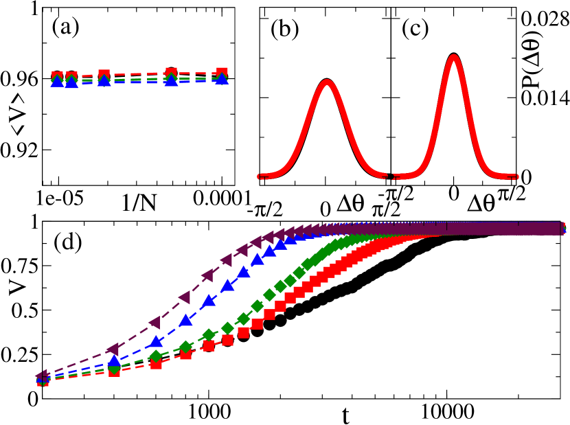
Figure 1: (Color online) (a) Plot of average global order parameter $\langle V\rangle$ vs. $1/N$ is shown for different $\sigma$. Black circles, red squares, green diamonds, and blue triangles are for $\sigma=0.0,0.001,0.01,$ and $0.05$, respectively. Error bars are less than symbol sizes. Plot of $P(\Delta\theta)$ of the SPPs at steady state for $\sigma=0.0$ and $0.05$ are shown in (b) and (c), respectively. Black and red circles are for $N=50000$ and $100000$, respectively. (d) The time series of $V$ is shown for different $\sigma$. Black circles, red squares, green diamonds, blue triangles up and maroon triangles down are for $\sigma=0.0,0.005,0.01,0.03$ and $0.05$ respectively. $N=50000$.

Ordered steady state:- In constant speed models or Vicsek like models Vicsek1995 ; Chateprl2004 ; Chatepre2008 ordered state exhibits a true long-range order in 2D. In general the ordering in the system is measured by calculating the global order parameter which is defined as

$$V(t)=\dfrac{1}{N}|\sum_{i=1}^{N}{\bf n}_{i}(t)|.$$ (3)

$V\sim 0$ for disordered state and it is close to 1 for completely ordered state. We start the simulation with random position and orientation of the SPPs, and with time, the system slowly evolves to the ordered state $V\sim 1$ for $\eta_{0}=0.2$. The $\langle V\rangle$ vs. $1/N$ plot is shown in Fig. 1 (a), where $\langle..\rangle$ denotes averaging over steady state time $5\times 10^{4}$ to $10^{5}$ and $10$ independent realizations. We note that $\langle V\rangle$ remains independent of system size $N$, therefore, one can safely show the LRO state even for finite value of $\sigma$. Furthermore, we calculate the probability distribution function (PDF) of the orientation of the particles $P(\Delta\theta)$ for different $\sigma$, where $\Delta\theta$ is the deviation in the orientation of the particles from the mean orientation direction. The width of $P(\Delta\theta)$ for non-zero $\sigma$ does not change with the system size $N$, as shown in Fig. 1(c). It further confirms the LRO state of the system in presence of the IS similar to the constant speed models as shown in Fig. 1(b). The plot of $V(t)$ vs. time $t$ is shown in Fig. 1(d) for four different values of $\sigma$ among the SPPs. The system takes less time to achieve the steady state with increasing $\sigma$. This behaviour of the system suggests that the IS among the SPPs accelerates the ordering in the system.

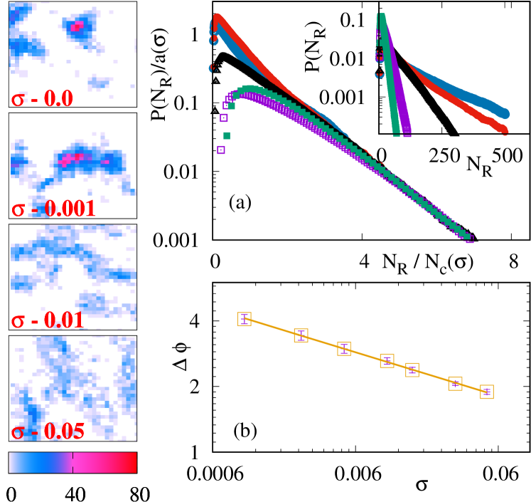
Figure 2: (Color online) Left column: Snapshots of the system in the steady state is shown for different $\sigma$. $N=20000$ and time $t=100000$. Color bar represents the number of particles in unit area. (a) Plot of $P(N_{R}/a(\sigma))$ vs. $N_{R}/N_{c}(\sigma)$ and $P(N_{R})$ vs. $N_{R}$ (inset) for different $\sigma$ is shown. Acme blue, red, black, violet, and teal color is for $\sigma=0.0,0.0005,0.001,0.01$ and $0.05$, respectively. $N=100000$. (b) Variation of $\Delta\phi$ vs. $\sigma$ is shown. Squares are numerical data, and solid line is the power law fitting of the numerical data with exponent $\sim-0.2$. Vertical lines shows the error bar. $N=50000$.

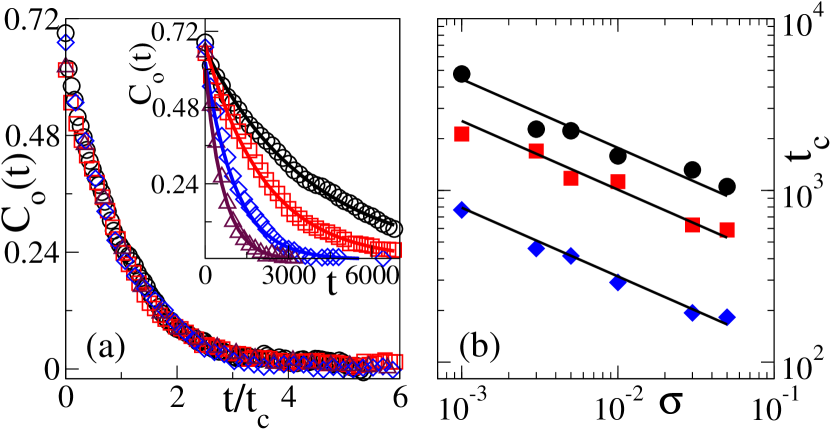
Figure 3: (Color online) (a) Plot of $C_{o}(t)$ vs. $t/t_{c}$ is shown for different $\sigma$. Inset: Variation of $C_{o}(t)$ with time $t$ is shown for different $\sigma$. Black circles, red squares, blue diamonds, and maroon triangles up, are for $\sigma=0.0,0.001,0.01$ and $0.05$, respectively. Solid lines in the inset are exponential fitting of the numerical data. Density of external agents $\rho_{a}=0.005$. (b) The variation of $t_{c}$ vs. $\sigma$ is shown for three different values of $\rho_{a}$. Black circles, red squares, and blue diamonds are numerical data points for $\rho_{a}=0.005,0.01$ and $0.05$, respectively. Black solid line is power law fitting with exponent $-0.4$ of the numerical data points. Error bars are less than the symbol size. $N=20000$.

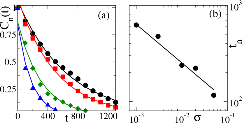
Figure 4: (Color online) (a) Plot $C_{n}(t)$ is shown for four different $\sigma$. Black circles, red squares, green diamonds, and blue triangles are for $\sigma=0.0,0.001,0.01,$ and $0.05$, respectively. Solid lines are the exponential fitting of the numerical data. (b) Plot of $t_{n}$ vs. $\sigma$ is shown. Black solid circles are numerical data and black solid line is the power law fitting of the numerical data with exponent $\sim-0.4$. Error bars are less than the symbol size. $N=50000$.

Properties of the flock state:- We have already seen that the system with IS exhibits a LRO state. However, the steady state features of the ordered state changes with increasing $\sigma$. In Fig. 2, we show the real space snapshots of the system for four different values of $\sigma(=0.0,0.001,0.01$ and $0.05$) at time $t=10^{5}$. In the constant speed model $\sigma=0.0$, particles form isolated clusters which move coherently in one direction. But these isolated clusters break down and the system becomes homogeneous with increasing $\sigma$. In the inset of Fig. 2(a), we plot the PDF of number of neighbors $P(N_{R})$ for different $\sigma$. $P(N_{R})$ vs. $N_{R}$ for $\sigma=0.0$ decays with a long tail, but the tail sharpens with increasing $\sigma$. Hence, average number of neighbors for each SPP decreases with $\sigma$. The plot of $P(N_{R})/a(\sigma)$ vs. $N_{R}/N_{c}(\sigma)$ is shown in Fig. 2(a) (main), where $N_{c}(\sigma)$ is obtained from the exponential fitting $a(\sigma)\times exp(-N_{R}/N_{c})$ of the tail of $P(N_{R})$ and $a(\sigma)$ is the pre-factor of the fitting function. To further confirm the effect of the IS on density clustering we calculate the density phase separation order parameter $\Delta\phi$ (the standard deviation of particles among the sub-cells). We calculate $\Delta\phi$ by dividing the whole $L\times L$ system into unit sized sub-cells. $\Delta\phi$ of the system is defined as:

$$\Delta\phi=\big{\langle}\sqrt{\dfrac{1}{L^{2}}\sum_{j=1}^{L^{2}}(\phi_{j})^{2}-(\dfrac{1}{L^{2}}\sum_{j=1}^{L^{2}}\phi_{j})^{2}}\big{\rangle},$$ (4)

where $\phi_{j}$ is the number of particles in each sub-cell and $\langle..\rangle$ represents averaging over $20$ realizations. We note that $\Delta\phi$ decreases with increasing $\sigma$ with a power $0.2$ as shown in Fig. 2(b). Hence, the system becomes homogeneous with increasing IS among the particles.
Inhomogeneous speed helps in faster information transfer:- We claim that the inhomogeneous speed distribution enhances the information transfer inside the flock, and a small number of quenched external agents are introduced in the system to characterize this behavior. In the presence of the external perturbation the SPPs slowly reorient themselves along the direction of the perturbation. Response of the flock to external agents is measured by direction auto-correlation function $C_{o}(t)$ of the SPPs:

$$C_{o}(t)=\langle cos(\theta_{i}(t)-\theta_{i}(0))\rangle,$$ (5)

where $\theta_{i}(t)$ and $\theta_{i}(0)$ are the directions of the $i^{th}$ particle at time $t$ and at the reference time $t=0$ (when the external agents are introduced). $\langle..\rangle$ denotes averaging over all the SPPs and $30$ different realizations. $C_{o}(t)$ shows an exponential decay $e^{-t/t_{c}}$ with time, as shown in Fig. 3(a)(inset). $t_{c}$ is the measure of time of a moving flock to reorient its direction along the external perturbation. Furthermore, we also note that the auto-correlation function shows an excellent scaling behaviour for different $\sigma$, as shown in the main Fig. 3(a). The correlation time $t_{c}$ decays with a power $\sim 0.4$ with increasing $\sigma$, as shown in Fig. 3(b). Therefore, the response of the flock to an external perturbation becomes faster for IS distribution. We also show that value of exponent remains invariant for different density of the external agents $\rho_{a}=0.005,0.01$ and $0.05$ in Fig3 (b).
Furthermore, we claim that the accelerated response is due to the more frequent update of neighbors for large IS. We calculate the change in neighbor list $Y(t)$ with time $t$ as defined in supplementary material (SM). We note that the neighbours list is updated more frequently for large IS. Furthermore, we calculate the time lag $t$ neighbor auto-correlation function

$$C_{n}(t)=\bigg{\langle}\dfrac{\sum_{t^{\prime}=1}^{T-t}(Y(t^{\prime})-\bar{Y})(Y(t^{\prime}+t)-\bar{Y})}{\sum_{t^{\prime}=1}^{T}(Y(t^{\prime})-\bar{Y})^{2}}\bigg{\rangle},$$ (6)

where $\bar{Y}$ is the mean value of $Y(t)$ over the total time $T$ and $t<T$ Box1976 . $\langle..\rangle$ represents averaging over $15$ independent realizations. Faster decay of $C_{n}(t)$ means more frequent update of neighbour list. We note that $C_{n}(t)$ decays exponentially $e^{-t/t_{n}}$ with time $t$ as shown in Fig. 4(a). In Fig. 4(b), the algebraic decay of $t_{n}$ (with a power $\sim 0.4$) is shown as a function of $\sigma$, which is similar to the variation of $t_{c}$ with $\sigma$, as shown in Fig. 3(b). The frequent update of neighbors of each SPP leads to the quicker information transfer. To confirm that the two quantities, $t_{n}$ and $t_{c}$, are related, we show the movies of the change in the neighbors list for a tagged particle and the response of the SPPs to the external perturbation for $\sigma=0.0,0.001$ and $0.01$ in sigma0 , sigma0.001 and sigma0.01 , respectively. The movies show that the SPPs slowly reorient along the direction of the external perturbation. The time required by the SPPs to orient along the external perturbation decreases on increasing $\sigma$. Also the neighbors of the particles change more frequently for large $\sigma$, therefore, both $t_{c}$ and $t_{n}$ decrease with the IS.
Conclusion:- We introduce a model for the collection of SPPs moving with the IS on a two-dimensional substrate, and such inhomogeneous systems are abundant in the nature. However, effect of such inhomogeneity is rarely studied in theory and simulations. In general the spatial inhomogeneity into Vicsek like models destroy the long-range ordering Chepizhko2013 ; Morin2017 . Surprisingly, our model with the IS preserves the macroscopic LRO state found in the homogeneous or the constant speed modelsVicsek1995 ; Chateprl2004 ; Chatepre2008 ; Toner1995 ; Toner1998 . Instead of destroying the LRO state, existence of the IS helps the system to reach the LRO state faster compared to the constant speed models or the Vicsek like models Vicsek1995 ; Chateprl2004 ; Chatepre2008 . Response of the flock to an external perturbation is measured by introducing a few orientationally and spatially quenched external agents.
We note that the IS of the SPPs enhances the response of the flock to the external perturbation. The flock state becomes homogeneous with increasing the strength of the IS ($\sigma$), and it is easier to bend the homogeneous cluster along the external perturbation. We show that the $t_{c}$ and $t_{n}$ decrease with increasing $\sigma$, larger $\sigma$ enhances the update in the neighbors and which in turn helps faster exchange of information inside the system.
Our model may be useful to understand the effect of the IS on collective behavior in natural systems like migrating birds or animals. Recently the experimental study by Lisicki et al. on unicellular eukaryotes, e.g., flagellates and ciliates, find that the probability distribution of swimming speed of the eukaryotes does not follow the constant speed model Lisicki2019 . We hope this work will convince more scientists to consider intrinsic inhomogeneity which helps in formation of flock state in active systems.
Acknowledgement:- We thank TUE computational facility at S.N.B.N.C.B.S.. S. Pattanayak thanks Sriram Ramaswamy for useful discussions and also thanks Department of Physics IIT (BHU), Varanasi for kind hospitality during the visit. S. Mishra thanks DST, SERB(INDIA), project no. ECR/2017/000659 for partial financial support.

References

- (1) T. Feder, Physics Today 60, 10, 28 (2007).
- (2) I. D. Couzin,, J. Krause, N. R. Franks, and S. A. Levin, Nature 433, 513–516 (2005).
- (3) A. Strandburg-Peshkin, C. R. Twomey, N. W. Bode, A. B. Kao, Y. Katz, C. C. Ioannou, S. B. Rosenthal, C. J. Torney, H. Wu, S. A. Levin, I. D. Couzin, Current Biology 23 (17), R709-711 (2013).
- (4) N. Miller, S. Garnier, A. T. Hartnett, and I. D. Couzin, PNAS 110 (13) 5263-5268 (2013).
- (5) J. E. Herbert-Read, Journal of Experimental Biology 219 2971-2983 (2016).
- (6) F. Ndlec, Ph.D. thesis, Universit Paris 11, 1998; F. Ndlec, T. Surrey, A. C. Maggs, and S. Leibler, Nature (London) 389, 305 (1997).
- (7) H. Yokota (private communication); Y. Harada, A. Noguchi, A. Kishino, and T. Yanagida, Nature (London) 326, 805 (1987); Y. Toyoshima et al., Nature (London) 328, 536 (1987); S. J. Kron and J. A. Spudich, Proc. Natl. Acad. Sci. U.S.A. 83, 6272 (1986).
- (8) J. T. Bonner, Proc. Natl. Acad. Sci. U.S.A. 95, 9355 (1998); M. T. Laub and W. F. Loomis, Mol. Biol. Cell 9, 3521 (1998).
- (9) D. Chen , Y. Wang, G. Wu, M. Kang, Y. Sun, and W. Yu, Chaos 29, 113118 (2019).
- (10) D. Helbing, I. Farkas, and T. Vicsek, Nature (London) 407, 487 (2000); Phys. Rev. Lett. 84, 1240 (2000).
- (11) Three Dimensional Animals Groups, edited by J. K. Parrish and W. M. Hamner (Cambridge University Press, Cambridge, England, 1997).
- (12) D. Helbing, I. Farkas, and T. Vicsek, Nature (London) 407, 487 (2000).
- (13) T. Vicsek, A. Czirk, E. Ben-Jacob, I. Cohen, and O. Shochet, Phys. Rev. Lett. 75, 1226 (1995); A. Czirk, H. E. Stanley, and T. Vicsek, J. Phys. A 30, 1375 (1997).
- (14) N. D. Mermin, and H. Wagner, Phys. Rev. Lett. 17, 1133–1136 (1966).
- (15) G. Grgoire and H. Chat, Phys. Rev. Lett. 92, 025702 (2004).
- (16) H. Chat, F. Ginelli, Guillaume Grgoire, and F. Raynaud Phys. Rev. E 77, 046113 (2008).
- (17) J. Toner and Y. Tu, Phys. Rev. Lett. 75, 4326 (1995).
- (18) J. Toner and Y. Tu, Phys. Rev. E 58, 4828 (1998).
- (19) A. Morin, N. Desreumaux, J. Caussin, and D. Bartolo, Nature Physics 13, 63–67 (2017).
- (20) O. Chepizhko, E. G. Altmann, and F. Peruani, Phys. Rev. Lett. 110, 238101 (2013).
- (21) D. Yllanes, M. Leoni, and M. C. Marchetti, New Journal of Physics 19, 103026 (2017).
- (22) D. A. Quint and A. Gopinathan, Phys. Biol. 12, 046008 (2015).
- (23) C. Sndor, A. Libl, C. Reichhardt, and C. J. Olson Reichhardt, Phys. Rev. E 95, 032606 (2017).
- (24) C. J. O. Reichhardt and C. Reichhardt, Nat. Phys. 13, 10 (2017).
- (25) R. Das, M. Kumar, and S. Mishra, Phys. R. E. 98, 060602(R) (2018).
- (26) J. Toner, N. Guttenberg, and Y. Tu, Phys. Rev. E 98, 062604 (2018).
- (27) J. Toner, N. Guttenberg, and Y. Tu, Phys. Rev. Lett. 121, 248002 (2018).
- (28) Guo-yuanWang, Fan-yu Wu, You-liang Si, Q. Zeng, and P. Lin, Procedia Engineering 211, 699 (2018).
- (29) G. A. Frank and C. O. Dorso, Physica A (Amsterdam, Neth.) 390, 2135 (2011).
- (30) A. Garcimartín, D. R. Parisi, J. M. Pastor, C. Martín-Gmez, and I. Zuriguel, J. Stat. Mech. 4, 043402 (2016).
- (31) I. Zuriguel, J. Olivares, J. M. Pastor, C. Martn-Gmez, L. M. Ferrer, J. J. Ramos, and A. Garcimartín, Phys. Rev. E 94, 032302 (2016).
- (32) I. Zuriguel, A. Janda, A. Garcimartín, C. Lozano, R. Arvalo, and D. Maza Phys. Rev. Lett. 107, 278001 (2011).
- (33) J. Hebner and D. Osborn, Kumbha Mela: The World’s Largest Act of Faith, Mandala Publishing Group (1991).
- (34) M. Specia, Hajj Begins as Muslims Flock to Mecca, The New York Times, Aug. 09, (2019).
- (35) M. Lisicki, M. F. V. Rodrigues, R. E. Goldstein, and E. Lauga1, eLife 8, e44907 (2019).
- (36) L. H. Cisneros, J. O. Kessler, S. Ganguly, and R. E. Goldstein, Phys. Rev. E. 83, 061907 (2011).
- (37) G. E. P. Box, and G. Jenkins, Time Series Analysis: Forecasting and Control, Holden-Day (1976).
- (38) Movie of a part of the system for is shown in the presence of external perturbation. Time is the reference time, when the external agents are introduced in the steady state. The orientation of the external agents is radians which is shown by a green arrow. The time span of the movie is after the external perturbation is applied to the system at the steady state. Time difference between two consecutive snapshots is . Cyan color represents the tagged particle. Circle represents the interaction radius of the tagged particle, and arrows indicate the direction of motion of the SPPs. Initially, the tagged particle is surrounded by the red particles and with time new neighbors appear (black particles). Also the direction of motion of the SPPs gradually changes along the external field ( radians). and .
- (39) Movie of a part of the system for is shown in the presence of external perturbation. Time is the reference time when the external agents are introduced in the steady state and orientation of the external agents is radians which is shown by a green arrow. The time span of the movie is after the external perturbation is applied to the system at the steady state. Time difference between two consecutive snapshots is . Colors, circle and arrows represent same as in sigma0 . Systems parameters are same as in sigma0 .
- (40) Movie of a part of the system for is shown in the presence of external perturbation. Time is the reference time when the external agents are introduced in the steady state and orientation of the external agents is radians which is shown by a green arrow. The time span of the movie is after the external perturbation is applied to the system at the steady state. Time difference between two consecutive snapshots is . Colors, circle and arrows represent same as in sigma0 . Systems parameters are same as in sigma0 .