Optical follow-up of gravitational wave triggers with DECam during the first two LIGO/VIRGO observing runs

Abstract

Gravitational wave (GW) events detectable by LIGO and Virgo have several possible progenitors, including black hole mergers, neutron star mergers, black hole–neutron star mergers, supernovae, and cosmic string cusps. A subset of GW events are expected to produce electromagnetic (EM) emission that, once detected, will provide complementary information about their astrophysical context. To that end, the LIGO–Virgo Collaboration (LVC) sends GW candidate alerts to the astronomical community so that searches for their EM counterparts can be pursued. The DESGW group, consisting of members of the Dark Energy Survey (DES), the LVC, and other members of the astronomical community, uses the Dark Energy Camera (DECam) to perform a search and discovery program for optical signatures of LVC GW events. DESGW aims to use a sample of GW events as standard sirens for cosmology. Due to the short decay timescale of the expected EM counterparts and the need to quickly eliminate survey areas with no counterpart candidates, it is critical to complete the initial analysis of each night’s images as quickly as possible. We discuss our search area determination, imaging pipeline, and candidate selection processes. We review results from the DESGW program during the first two LIGO–Virgo observing campaigns and introduce other science applications that our pipeline enables.

1 Introduction

A particular challenge for precision cosmology is the absolute calibration of cosmic distances. Traditionally, it employs a cosmic distance ladder: direct geometrical parallax measurements of nearby stars that calibrate indirect measurements for larger distances, in a series of steps extending to cosmological scales (Riess et al., 2019). This indirect approach introduces systematic uncertainties to measurements from type-Ia supernovae and other probes. Gravitational wave (GW) signals from merging binary objects, however, act as standard sirens, enabling distances to be measured directly to the source without relying on a cosmic distance ladder (Schutz, 1986; Holz and Hughes, 2005; Del Pozzo, 2012). This fact motivates the pursuit of a cosmology program using GW events. The results reported by the LIGO–Virgo Collaboration (LVC) in their first observing run with an advanced interferometer network included detection of binary black hole (BBH) mergers at $440^{+180}_{-190}$ (Abbott et al., 2016a) and $420^{+160}_{-180}$ (Abbott et al., 2016b) Mpc, proving that the current generation of interferometers are sensitive enough to observe mergers at cosmological distances.

Anticipating that such sensitivity would be in reach, the Dark Energy Survey (DES) launched its GW program (DESGW) in the first LVC run (O1, 2015–2016). DESGW is a search and discovery program for electromagnetic (EM) signatures of GW events. While there are multiple reasons to search for GW electromagnetic counterparts, our primary goal is to perform a measurement of the Hubble Constant with the best precision afforded by the available data. The second LVC run (O2, 2016–2017) saw the observation of a binary neutron star (BNS) merger (Abbott et al., 2017a) and DESGW contributed (Soares-Santos et al., 2017) to the discovery of its EM counterpart (Abbott et al., 2017b). The third run (O3, 2019–2020) is ongoing at the time of this writing. The DESGW cosmology program has two different components: 1) If the GW signal has an EM counterpart, the location of the event may be identified to the arcsecond and a redshift for the galaxy obtained. 2) If the GW counterpart is electromagnetically dark, then the redshift must be obtained statistically using all the galaxies in the probable localization volume of the event.

In this article we detail, for the first time, the DESGW observational program to search for EM counterparts of GW events in the optical range using the Dark Energy Camera (DECam). DESGW has been active during all three LVC observing runs to date and we document changes implemented from one run to another. We begin this article with a discussion of cosmology with standard sirens (Section 2), and then describe DECam itself (Section 3), along with how the decision to trigger on a given GW event is made, including the interaction with other telescope users. Section 4 describes the experimental setup, and Section 5 describes our overall observing strategy and construction of a detailed observing plan for each night. Sections 6 though 8 discuss our image processing pipeline and final candidate selection. We conclude with a brief review of DESGW results from the first two observing seasons in Section 9 and a discussion of planned improvements to our program and other science applications in Section 10.

2 Cosmology with standard sirens

2.1 Bright Standard Sirens

Mergers for which both gravitational and electromagnetic emission are detectable, bright standard sirens, can be used to determine cosmological parameters such as $H_{0}$ via the distance-redshift relation: the distance measurement comes from the GW signal and the redshift from identifying the host galaxy of the EM counterpart. Mergers of neutron stars, or of a neutron star and a black hole, have multiple predicted signatures (Metzger et al., 2010; Nissanke et al., 2010; Gaertig et al., 2011; Berger, 2014; Metzger, 2017; Rosswog et al., 2017; Tanaka et al., 2018; Gottlieb et al., 2018; Paschalidis and Ruiz, 2019; Duque et al., 2019): a gravitational wave chirp, a neutrino burst, a gamma-ray burst followed by an afterglow in various wavelengths, and an optical transient referred in the literature as a kilonova, which we aim to detect with DECam. Fainter, redder, and shorter-lived than supernovae, kilonovae are challenging from the observational point of view. They are detectable mostly in red/infra-red wavelengths and only for about 1 or 2 weeks in an instrument such as DECam. With only one kilonova associated to a GW event so far, light-curve models (Metzger and Berger, 2012; Barnes and Kasen, 2013; Tanaka and Hotokezaka, 2013; Grossman et al., 2014; Metzger, 2017; Rosswog et al., 2017; Radice et al., 2018; Gompertz et al., 2018; Fahlman and Fernández, 2018; Bulla, 2019) are still very uncertain. They predict, for example, a wide range of peak magnitudes: e.g. $r$-band (650nm) magnitude 20–22 at a distance of 200 Mpc.

2.2 Precision Cosmology

$H_{0}$ is a powerful tool for precision cosmology which aims at characterizing the Universe as a whole: physics at the early times, history of expansion, and behavior of perturbations. With a distance-based measurement, we probe the history of expansion and are sensitive to dark energy models (often described in terms of the equation of state parameter $w=p/\rho$). Discrepancies between $H_{0}$ values determined from the Cosmic Microwave Background and from distance probes can be reconciled by allowing some of these model parameters to vary.

Uncertainties in $H_{0}$ measurements from standard sirens will depend, in part, on uncertainties achieved by the LVC network for the distance to each merger. According to a study (Nissanke et al., 2013) of simulated binary neutron star mergers, with a distance distribution and detector performance model that are representative of the third and fourth observing runs, an uncertainty of 3–5% on $H_{0}$ is expected for sample sizes of about 15–20 events. Similarly, for dark sirens, or GW events without an identified electromagnetic counterpart where the redshift must be obtained statistically (MacLeod and Hogan, 2008), simulations following the methodology of Soares-Santos & Palmese et al. (2019) estimate that 5% precision is achievable with a sample of 100 events (see also Chen et al. 2018 and Nair et al. 2018 for other estimates of the achievable precision on $H_{0}$ via standard sirens). After approximately 100 dark siren events and 20 bright siren events, we expect that our program can contribute to the $H_{0}$ discrepancy issue with a completely independent measurement at the $2\sigma$ level, a remarkable result for a brand new cosmological tool.

3 The DECam System

We use the Dark Energy Camera (Flaugher et al., 2015). DECam is a 570 Mpixel, 3-square-degree field-of-view camera with an active-pixel fill-factor of 0.8. It consists of 62 red-sensitive CCDs and a wide field of view corrector, all installed on the 4-meter Victor M. Blanco telescope at the Cerro Tololo Inter-American Observatory (CTIO). This sensor system is connected to a data reduction pipeline with computation hardware at the National Center for Supercomputing Applications (NCSA).

3.1 The DES, DECam, and the Community

The Dark Energy Survey Collaboration (DES) designed and constructed DECam with the primary goal of studying the nature of dark energy using four complementary probes: galaxy clusters, weak lensing, Type Ia supernovae, and baryon acoustic oscillations. As we have seen, precision measurements of $H_{0}$ are intricately linked with dark energy itself, thus our GW program complements the main DES probes. The camera was installed in 2012, significantly upgrading the Blanco telescope, completed in 1976. The high level requirements on the DECam design were driven by the need to visit a 5000 sq. deg. wide-survey area (the DES footprint) and a 30 sq. deg. supernova survey area over five years, with excellent image quality, high sensitivity in the near infrared, and low readout noise.

3.2 Template Coverage

Our transient discovery pipeline uses the “image differencing”technique. This technique works by comparing a search image to one or more images previously taken of the same area of sky (these images are called “templates”) and subtracting the template(s) from the search image. The result, known as the “difference image”, should consist only of objects not present in the template images, which are thus potential candidates to be an optical counterpart of the GW trigger. Inside the DES footprint, template images are always available, either from the DES wide-survey program or from other programs with publicly accessible data. Outside the DES footprint we rely on public images taken by other programs using DECam to provide templates. This method results in incomplete sky coverage (e.g. Fig. 1), illustrating the need for programs to complete the southern sky coverage, such as the Blanco Imaging of the Southern Sky (BLISS) survey. We require a minimum exposure time of 30 seconds in our templates, and our standard observing conditions requirements translate to effective magnitudes of 21.23 (20.57) for 30-second $i$ ($z$)-band images. Currently DECam public image coverage to this depth exists over approximately 59% (65%) of the accessible sky in the $i$ ($z$) band. If no template images pass the standard observing criteria we can loosen them as needed (though we retain the 30-second minimum) at the expense of search sensitivity (we are limited by the combined template depth), resulting in increased coverage. If no DECam template image was available at a given location we relied on so-called “late-time” images taken well after the event as templates. Late-time templates are non-optimal for two reasons: first, any residual light from the event in the late-time image systematically affects measured magnitudes of the event at earlier times. Second, the use of late-time template delays complete spectroscopic response until after the template is taken.

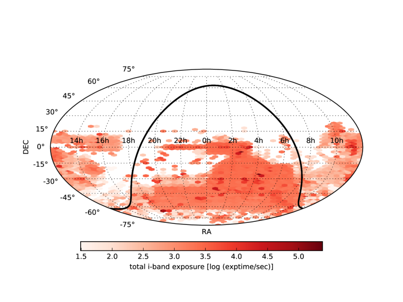
Figure 1: Existing $i$-band coverage of the sky from DECam imaging as of March 2019.

3.3 How the Interrupt Process Worked During DES Time

The first two LIGO observing runs coincided almost exactly with DES observing seasons. The DESGW group, consisting of members of the DES, LVC, and other members of the astronomical community, was awarded $\sim 4$ nights of telescope time per year via the open proposal process. DES and the DESGW entered into an agreement where the DESGW nights were added to the DES observing time allocation. If a trigger occurred, the DESGW and DES management teams consulted and if the event was judged interesting the DESGW interrupted the DES and made observations of the LIGO spatial localization. If the time was not used, the nights counted against the total night allocation of the DES.

4 The Experimental Setup

Figure 2 provides an overview of the experimental setup. The reception of a GCN trigger from LIGO triggered a three-part DESGW process. First, we calculated the possible coverage of the LIGO event with the DECam system for the next night and discussed whether to proceed with observations as previously described. If the decision was to interrupt and observe, we moved to the observation and data preparation phase. The observing team was briefed and provided the observing plan, and the template determination and preparation began. We make an initial determination of possible template overlaps based on our observing plan, discussed in detail in Sec. 5.

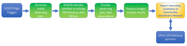
Figure 2: Overview of search program (green boxes are specific to this work). Our automated system continuously listens to the LIGO/Virgo data stream via GCN protocol. For a given trigger, an automated strategy code formulates the observing plan which we send to astronomers at the DES/DECam site to execute. We monitor the DECam data stream for new incoming images and automatically process them through the image differencing

pipeline.

The third phase is data reduction. During O1 and O2, the DESGW program aimed to process and analyze a given night’s observations within 24 hours so that we can report electromagnetic counterpart candidates to other telescopes for followup. We rapidly provision the required computing resources using a mixture of computing resources at Fermilab and a variety of other campus and laboratory sites via the Open Science Grid (OSG;  Pordes et al. 2007), relying on the high throughput of the OSG. As new search images arrive at Fermilab from CTIO via NCSA, the corresponding image processing jobs are sent to all available resources. The results are copied to local disk at Fermilab and summary data recorded in a database for postprocessing and candidate selection.

5 DESGW Observing: Map Making and Observing

Our system listens to the LIGO/Virgo alert stream. The MainInjector code initiates action on triggers by alerting DESGW team members and preparing initial observation maps. The observing scripts are generated by calculating event counterpart visibility probability maps summed inside an all-sky DECam hex layout and choosing the highest-probability hexes for highest priority observations.

We wish to calculate maps of

$$p(\alpha,\delta)=\int p(x|\alpha,\delta)p(y|\alpha,\delta)p(d|m,t,\alpha,\delta)dm\,.$$ (1)

where

• $p(x|\alpha,\delta)$ is the LIGO spatial localization map probability per pixel ($x$),

• $p(y|\alpha,\delta)$ is our ability to recognize the detection given source crowding and is related to a false positive rate,

• $p(d|m,t,\alpha,\delta)$ is the DECam detection probability of a source of magnitude $m$ at time $t$ per pixel, and

• the time dependence of $m$ enters via the source model.

We will discuss each of these items in turn.

(a) DES source probability time slot 1

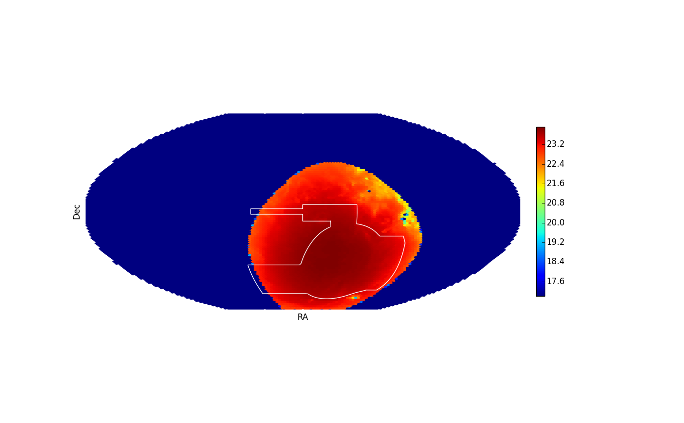
(b) Limiting magnitude map time slot 1

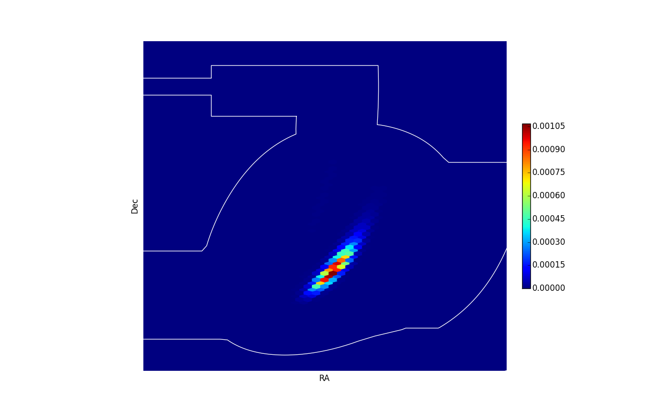
(c) DES $\times$ LIGO probability time slot 1

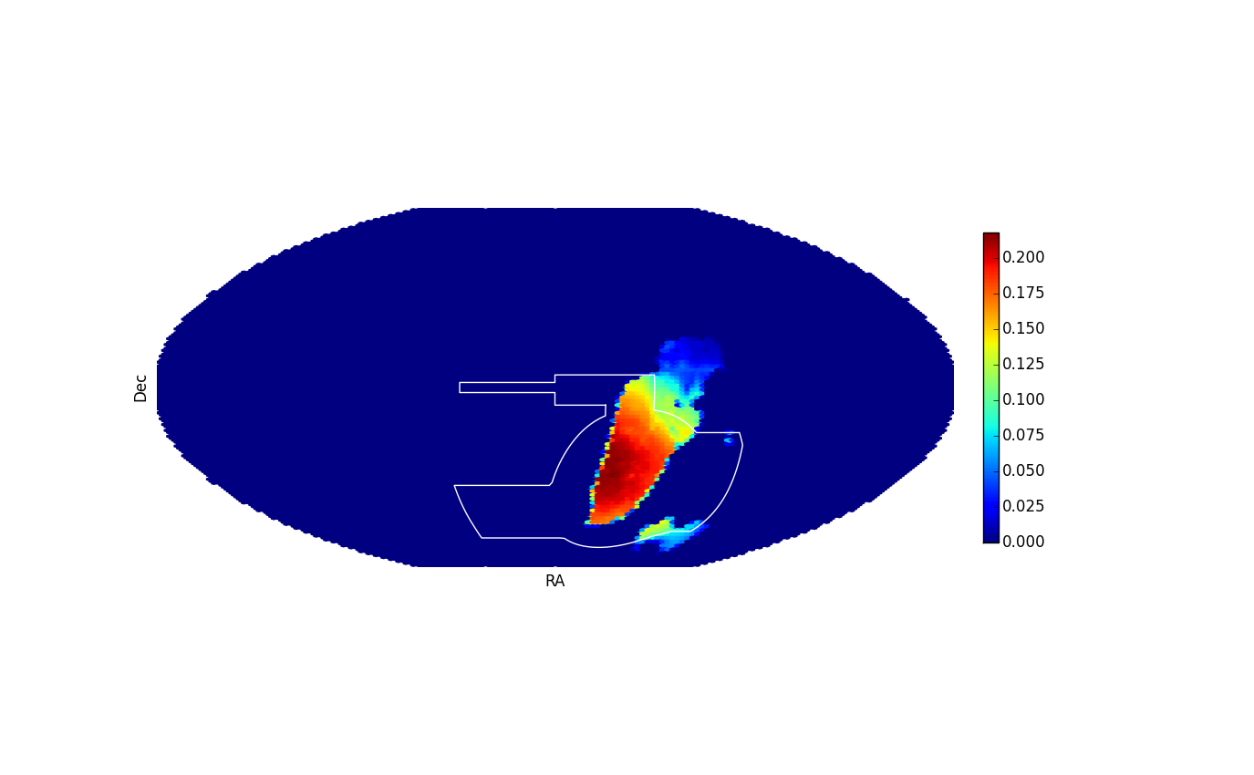
(d) DES source probability time slot 2

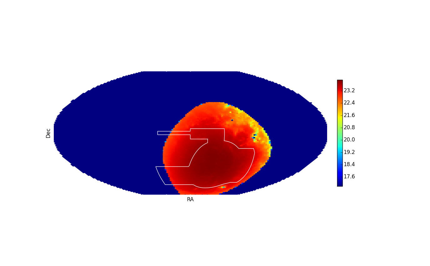
(e) Limiting magnitude map time slot 2

(f) DES $\times$ LIGO probability time slot 2

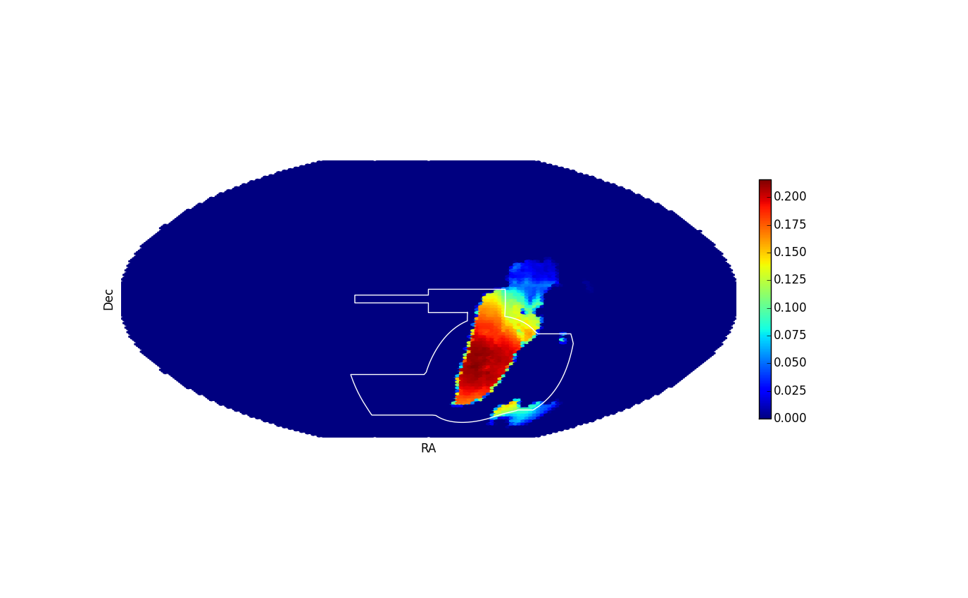
(g) DES source probability time slot 3

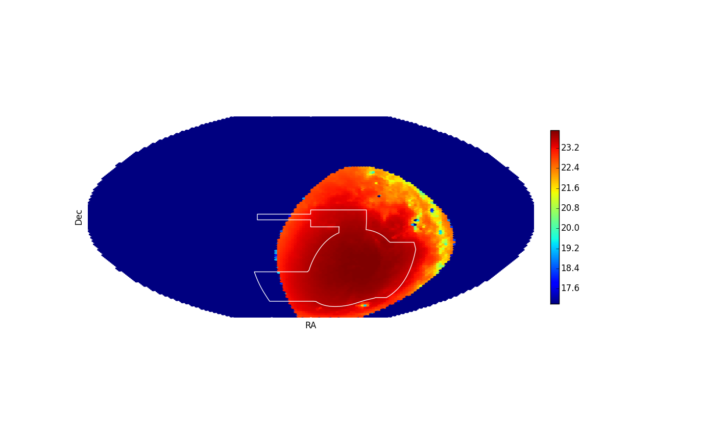
(h) Limiting magnitude map time slot 3

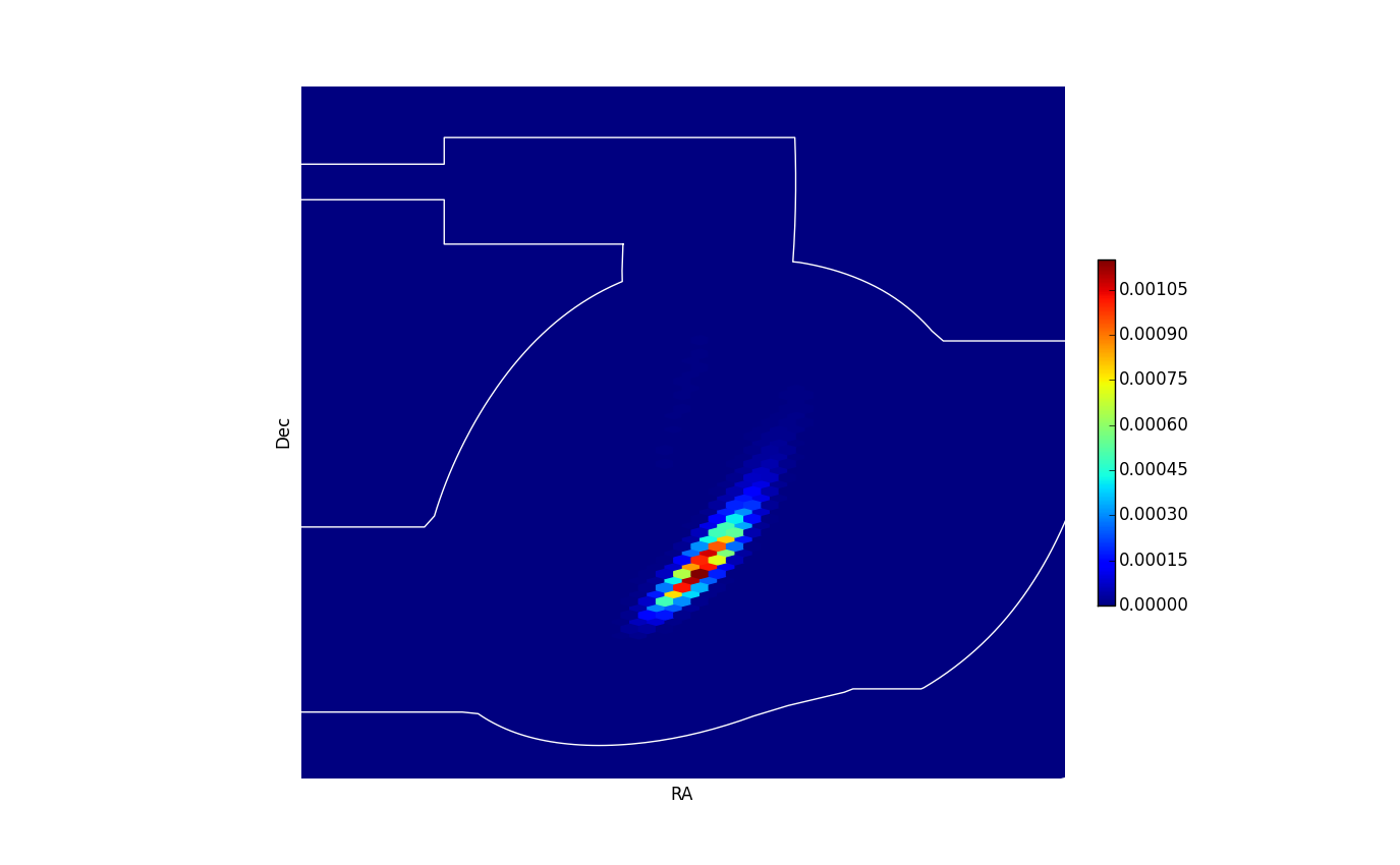
(i) DES $\times$ LIGO probability time slot 3

Figure 3: Source detection probability map construction.. We show the relevant probabilities and maps for three different time periods on a given night. While the source probability map is fixed (3(a),3(d),3(g)), the limiting magnitude map (3(b),3(e),3(h)), and thus the overall source detection probability map (3(c),3(f),3(i)), changes with time due to observing conditions and the Earth’s rotation. The example shown here is for GW170814, a binary black hole merger. The white contour represents the DES footprint.

5.1 Spatial Localization: $p(x|\alpha,\delta)$

LVC triggers include localization maps in HEALPix format (LIGO maps: Singer et al. 2016, HEALPix: Górski et al. 2005). The first of these maps provides the spatial localization probability per pixel, the second provides distance, the third provides a gaussian variance estimate on the distance, and the fourth contains a normalization plane. We take the first map to be $p(x|\alpha,\delta)$. Maps derived from this one have the same resolution as we choose to read this map.

5.2 Detection recognition probability map: $p(y|\alpha,\delta)$

We model $p(y|\alpha,\delta)$, the probability of recognizing a detection $y$ given source crowding, as a false positive rate problem related to the per-pixel stellar density and independent of magnitude. Essentially, if the targeted region is too full of stars then it is likely there will be too many false positives masking possible candidates, resulting in missed detections of real astrophysical transients. Our model is that the recognition probability is taken to be $p(y|\alpha,\delta)$ = 0.0 at or above 610 stars/deg² (roughly that of the Galactic anticenter) and $p(y|\alpha,\delta)$ = 1.0 at or below 10 stars/deg² (roughly that of the south Galactic pole), linear in surface density between. We use the 2MASS J-band star counts in units of stars/deg², cut at $J<16.0$, from the NOMAD catalog (Zacharias et al., 2004). Figures 3(a), 3(d), and 3(g) show example detection recognition probability maps for a given event.

5.3 Limiting magnitude maps

The calculation of $p(d|m,t,\alpha,\delta)$ proceeds through limiting magnitude maps, some examples of which are shown in Figs. 3(b), 3(e), and 3(h). A point source with intrinsic flux $f$ and full width half max $w$ that is faint compared to a sky background flux $s$ has a signal to noise S/N given by

$$S/N\propto\frac{T_{d}T_{a}ft}{w\sqrt{st}}=\frac{T_{d}T_{a}f\sqrt{t}}{w\sqrt{s}}$$ (2)

where $T_{d}$ is the transmission of light through a layer of Galactic dust, and $T_{a}$ is the transmission of light through the Earth’s atmosphere. We demand S/N=10 for a detection as $10\%$ flux uncertainties permit reasonable colors to be formed.

We define a fiducial set of conditions and a 90 sec DECam exposure to calculate the $10\sigma$ $i$-band magnitude, $m_{i}$, and use eq 2 to compute the limiting magnitude $m_{l}$ using $\Delta m$ to account for variations from the fiducial values:

$$\begin{split}m_{l}&=m_{i}+\Delta m\\ \Delta m&=2.5\log\left[\left(\frac{T_{d}}{T_{ncp}}\right)\left(\frac{T_{a}}{T_{1.3}}\right)\left(\frac{0.9^{\prime\prime}}{{\mathrm{F}WHM}}\right)\right]\\ &+\frac{1}{2}(m_{sky}-22.0)\end{split}$$ (3)

where $T_{ncp}$ is the transmission of dust at the North Celestial Pole, and $T_{1.3}$ is the transmission of the atmosphere at an airmass of 1.3, our fiducial value. This quantity is entirely a function of time of the observation: $T_{a}$ depends on zenith distance; the full width of half maximum of the PSF, $\mathrm{FWHM}$, depends on zenith distance; $m_{sky}$ depends on zenith distance, the lunar phase and position, and the solar position.

Transmission due to Galactic dust: The Planck dust map comes as a HEALPix map, with the values of the pixels being the optical depth $\tau$ at 350 $\mu$m multiplied by a normalization to convert to $E(B-V)$, the reddening. This is best understood as $A_{B}-A_{V}$, where the $A$ is the extinction in a given filter. The extinction in the $i$-band, $A_{i}$, is therefore $R_{i}\times E(B-V)$, where $R_{i}$ is the reddening coefficient for the $i$-band. The transmission due to dust, $T_{d}$, is $\log_{10}(T_{d})=0.4\cdot R_{i}\cdot E(B-V)$ so the transmission relative to the fiducial is thus

$$\begin{split}\log_{10}(T_{d})&=0.4\cdot R_{i}\cdot E(B-V)\\ \log_{10}(T_{ncp})&=0.4\cdot R_{i}\cdot E(B-V)_{ncp}\\ \log_{10}\left(\frac{T_{d}}{T_{ncp}}\right)&=0.4R_{i}[E(B-V)-E(B-V)_{ncp}]\end{split}$$ (4)

We take $E(B-V)_{ncp}$ to be 0.0041.

Atmospheric transmission: In a very simple model the transmission due to the atmosphere can be described as

$$\frac{T_{a}}{T_{a,f}}=\frac{10^{-0.4k_{i}X}}{10^{-0.4\cdot 1.3k_{i}}}=10^{-0.4k_{i}\left(X-1.3\right)}$$ (5)

where $k_{i}$ is the (first order) atmospheric extinction in the $i$-band, and $X$ is the airmass. Since zenith distance could be close to $90^{\circ}$ in our case, depending on the target of interest, we do not use the $X=\sec(zd)$ approximation to airmass, but the approximation due to Young (1994), which has a maximum error of 0.004 at $zd=90^{\circ}$.

$$X=\frac{a\cos^{2}(zd)+b\cos(zd)+c}{\cos^{3}(zd)+d\cos^{2}(zd)+e\cos(zd)+f}$$ (6)

where $a=1.002432$, $b=0.148386$, $c=0.0096467$, $d=0.149864$, $e=0.0102963$, and $f=0.000303978$.

The full width half max of the psf: $\mathrm{FWHM}$ is, statistically, a filter-dependent power law in zenith distance.

$$\frac{\mathrm{FWHM}}{\mathrm{FWHM}_{f}}=\left(\frac{\lambda}{\lambda_{f}}\right)^{-0.2}\left(\frac{X}{1.3}\right)^{3/5}$$ (7)

The sky surface brightness: The sky surface brightness model is from Krisciunas and Schaefer (1991), which predicts the sky brightness as a function of the moon’s phase and zenith distance, the zenith distance of the sky position, the angular separation of the moon and sky position, the local extinction coefficient, and the airmass of the sky position. Telescopes have software and hardware limits on their ability to point, which we model as a top hat on sky brightness: outside the pointing range the sky brightness is set arbitrarily high (the brightness of the full moon). We create this brightness map by converting the CTIO-provided Blanco HA,$\delta$ telescope limits into a HA,$\delta$ map.

5.4 Source detection probability: $p(d|m,t,\alpha,\delta)$

The calculation of the map $p(d|m,t,\alpha,\delta)$ uses the limiting magnitude map, the source model, and the LIGO event distance map. Discussion of the source model is in the next subsection and here we assume that model gives us an absolute magnitude $M$ and a model uncertainty dispersion of $\sigma_{M}$. We pursue the following calculation.

We convert the distance estimate from the LIGO trigger into a distance modulus $\mu=5\log r+25$, where the distance $r$ is in Mpc, and the distance uncertainty into an uncertainty on $\mu$:

$$\sigma^{2}=\sigma_{r}^{2}\left(\frac{5}{r\ln 10}\right)^{2}$$ (8)

Then the apparent magnitude of the source, $m_{s}$ is

$$m_{s}=M+\mu$$ (9)

and, as gaussians can be added to form gaussians,

$$\sigma_{m}^{2}=\sigma_{M}^{2}+\left(\frac{5}{r\ln 10}\right)^{2}\sigma_{r}^{2}$$ (10)

The resulting gaussian is normalized: $\int_{0}^{\infty}G(m_{s},\sigma_{m}^{2})dm=1$. The probability that the object could be seen in this pixel given a limiting magnitude of $m_{l}$ is then

$$p(d|m_{l},m_{s},\sigma_{m})=\int_{0}^{m_{l}}G(m_{s},\sigma_{m}^{2})dm$$ (11)

If $m_{s}>m_{l}$, then $p(d)={\mathrm{efc}}(m_{s}-m_{l})/2$. If $m_{s}<m_{l}$, then $p(d)=(1+{\mathrm{efn}}(m_{s}-m_{l}))/2$. The probability is weighted as uniform in volume: $\int p(d)dr=\int G(m_{s},\sigma_{m}^{2})r^{2}dr$. We will need to do the same weighting in apparent magnitude space, by transforming $r^{2}$ into distance modulus

$$r=10^{0.2(m-m_{s})-5}=10^{0.2(m-m_{s})+C}$$ (12)

$$r^{2}dr=C\,10^{0.6(m-m_{s})}dm$$ (13)

where $C$ is a constant. Then

$$\int_{0}^{r}Gr^{2}dr=C\int_{0}^{m_{l}}\exp\left(\frac{(m-m_{s})^{2}}{\sigma_{m}^{2}}\right)10^{0.6(m-m_{s})}dm$$ (14)

where $C$ is a normalization constant. This last equation is the probability that we will see a source given the model uncertainty and distance uncertainty for a known limiting magnitude and thus is $p(d|m,t,\alpha,\delta)$: recall $d$ here is a detection, $m_{l}$ is a function of spatial pixel ($\alpha,\delta$) and time ($t$) as described in Sec. 5.3, and $m_{s}$ depends on $M$, its uncertainty, and time as described in the next subsection.

5.5 The source model

The source model governs the source magnitude and uncertainty as a function of time. We operate with two theoretical source models, one for binary black hole mergers and one for mergers including a neutron star.

Our source model for BBH mergers is relatively arbitrary, as there is no well-motivated theoretical model. We assume simply that the counterpart has a falling $t^{-1}$ lightcurve: the source has an initial $i$-band magnitude of approximately 20 for a day or two, then fades below our typical detection thresholds for 90-sec exposures. Our source model for a merger involving a neutron star is more complicated. In O1 and O2, before detection of the BNS event GW170817, we were following the kilonova model of Barnes and Kasen (2013) and Barnes et al. (2016).

Briefly, as neutron stars merge, tidal tails grow into the equipotential surface and then mostly flow back into the main remnant. Some few percent of matter in the tails are dynamically ejected at speeds $\approx$ 0.1c. The ejected material undergoes r-process nucleosyntheis as the few nuclei in the sea of neutrons grow by neutron absorption. During O1 and O2 the details of our model followed the simulation-based analysis of Grossman et al. (2014). Observationally, we modeled the merger event luminosity, $L$, and temperature, $T$, and assumed the event is an optically thick blackbody of which we observe a photosphere. All the thermal energy available for comes from the the r-process beta-decay episode and we define an energy deposition rate per unit mass, $\epsilon$, so that $L\approx m\epsilon$. At early times ($t<t_{peak}$) $L$ scales as $L\propto t^{2}$ and at late times as ($t>t_{peak}$) $L\propto t^{-1/3}$. The time to peak brightness $t_{p}$ is $\sim m^{-1/2}$. We assume the photosphere is a blackbody $T=\left(\frac{L}{\sigma\left(2\sqrt{\pi}vt\right)^{2}}\right)^{0.25}$, where $vt$ came from the radius of the photosphere. The flux through any filter is then: $f=4.4\times 10^{22}\,\,\int B_{\lambda}{\rm d}\lambda\,\,L_{40}T_{1000}^{-4}d_{100}^{-2}$ where $L_{40}$ is the luminosity in units of $10^{40}$ ergs/sec, $T_{1000}$ is the temperature in units of $1000$ K, and $d_{100}$ is the distance in units of 100 Mpc.

We can break up the model into sub-components, each of which has a different opacity. In our model we use a Barnes and Kasen iron model $(\kappa\approx\ 0.1)$ and an Barnes and Kasen lanthanide model $(\kappa\approx\ 10)$. We use the same energetics as described above; one swaps out the $B_{\lambda}$ for a computed SED as one computes the flux through a filter.

There was a range of uncertainties in the peak absolute magnitudes. For a given time we calculate the model absolute magnitude, $M$ which has a model uncertainty dispersion of $\sigma_{M}$.

During and after the intensive observations of the counterpart to GW170817, better models have been developed, for example the three-component model of Villar et al. (2017). It was unclear whether there would be a blue component before the observations of GW170817; in the work described here we assumed only a red component and a generally fainter absolute magnitude than the counterpart of GW1701817 exhibited. We have updated the kilonova model implementation in our O3 pipeline.

5.6 Observing plan construction

Once we have calculated maps of $p(\alpha,\delta)$ we can construct the observing plan. Each observation is of a hex, so named because the DECam focal plane is roughly hexagonal. An observation may be a single 90s $i$-band exposure, as in BBH sources, or a triplet of 90s each in an $i,z,z$ band sequence, as in events containing NS. The aim is different in each case. For NS we are looking for the week-timescale very red transient that is the signature of kilonova. For BH we are assuming a source similar to a $t^{-1}$ power law and attempting to build light curves that allow us to reject supernovae.

To construct the plan we create slots of time that contain integer numbers of hexes with a total duration of around a half hour; each slot has the full map-making performed. For NS events there are six hexes per slot (three 90s observations per hex), while for BH and bursts, there are 18 hexes per slot (one 90s observation per hex). The detection probability maps (e.g. Figs. 3(c), 3(f), 3(i)) are then “hexelated”: the probabilities are summed inside a fixed pattern of camera pointings. For the night, the hex with the greatest probability is found and assigned to be observed in a time slot. The time slot is chosen to maximize the observability of the hex in question (and probability of actual detection of the transient if it happens to be located in those exposures). That hex is then removed from consideration (removing all probabilities for that hex at different time slots in the night), and we repeat the procedure with the next-highest probability hex until all slots are full. We use a mean overhead time of 30s between hexes to account for the time it takes to move the telescope from one position to another. Now we have a time series that makes full use of observing probabilities, aiming to ensure we observe as many high-probability hexes as possible on a given night, and following an optimal sequence, as shown in Figure 4. We convert this list to a JSON file with the appropriate content to drive DECam and the Blanco telescope. The same JSON files, modified for a later time, are used during the subsequent observing nights.

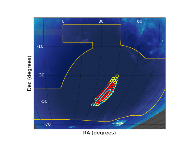
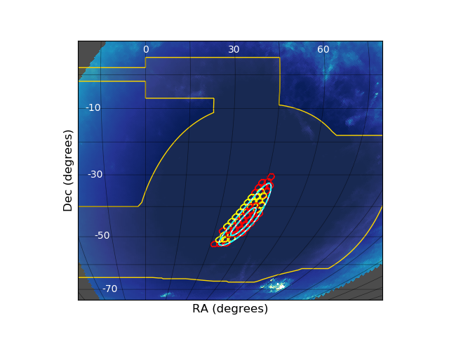
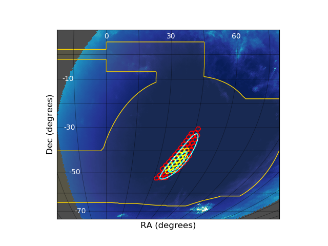
Figure 4: Final observing plan for three time slots based on the source detection probability maps in Figs. 3(c), 3(f), and 3(i)). The red hexagons are all scheduled observations across all slots, while the yellow hexagons are those performed within the given time slot. The solid white lines are the 50% and 90% LIGO probability contours, and the yellow line represents the nominal DES footprint. The example shown here is for GW170814, a binary black hole merger.

6 Image processing pipeline: images to candidates

We build on the existing DES image processing pipelines. For image preparation we use the DES single-epoch (SE) processing pipeline (Morganson et al., 2018). We use a modified version of the DES supernova processing pipeline (DiffImg), described in Kessler et al. (2015), to perform image differencing. This pipeline has a strong track record of discovering rare classes of transient and rapidly fading objects such as in Pan et al. (2017) and Pursiainen et al. (2018). We give a description of both pipelines here, focusing on the modifications made specifically for DESGW.

6.1 Single-epoch processing

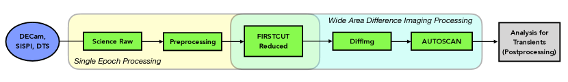
Figure 5: A schematic view of the modules and steps in the DESGW pipeline (shaded area marked “Wide Area Difference Imaging Processing”). Calibration and raw science images are delivered from DECam to NCSA. In single-epoch processing (yellow box), raw science exposures undergo preprocessing before proceeding to the DiffImg stage (blue box). Diagram based on Figure 3 of Morganson et al. (2018).

The first stage of image processing each night is the SE pipeline, which consists of an image correction stage (6.1.1) and an object cataloging stage known as FirstCut (6.1.3), which includes astrometric calibrations (described separately in 6.1.2).

6.1.1 Image Correction

SE begins with a stage to make the raw images science-ready. This stage includes crosstalk corrections, pixel corrections, and bad pixel masking (Bernstein et al., 2018). The pixel corrections include bias subtraction, pixel non-linearity correction, a conversion from DN to electrons, a “brighter-fatter” correction, and finally flat fielding. This stage creates a catalog of the brighter objects in each image with SExtractor (Bertin, 2011), to be used in the astrometric calibration (described in Section 6.1.2).

6.1.2 Astrometric Calibration

The astrometry stage uses SCAMP (Bertin, 2006) with the aforementioned catalog of bright objects, generated by SExtractor during image correction, to calculate an astrometric solution using an initial-guess of third-order polynomial World Coordinate System (WCS; Greisen and Calabretta 2002) distortion terms for each of the 62 CCDs in the DECam array to produce a solution to place CCD pixel positions into a TPV WCS. During O1 and O2 we used the 2MASS point source catalog (Skrutskie et al., 2006) to solve for the entire focal plane solution for every DES pointing. We have typical (RMS) DES-2MASS differences of $0.25^{\prime\prime}$. These errors are dominated by 2MASS which has typical single detection uncertainties of $0.2^{\prime\prime}$ for sources fainter than $K_{S}$ of 14. An improvement during the third observing season is to use the Gaia catalog (Gaia Collaboration et al., 2016; Lindegren et al., 2018) as a reference, allowing both reduction of DES astrometric uncertainties to below $0.03^{\prime\prime}$ per coordinate (dominated by DES uncertainties) and for us to calculate an astrometric solution CCD by CCD rather than over the whole image. Per-CCD calculations can run in parallel and are much faster.

6.1.3 FirstCut

The FirstCut processing calculates an astrometric solution with SCAMP (see 6.1.2), performs bleed trail masking, fits and subtracts the sky background, divides out the star flat, masks cosmic rays and satellite trails, measures and models the point spread function (PSF), performs object detection and measurement using SExtractor, and performs image quality measurements.

To catalog all objects from single-epoch images we run SExtractor using PSF modeling and model-fitting photometry. A PSF model is derived for each CCD image using the PSFEx package (Bertin, 2011). We model PSF variations within each CCD as a $N^{\mathrm{th}}$ degree polynomial expansion in CCD coordinates. For our application we adopt a $26\times 26$ pixel kernel and follow variations to 3^rd order.

In SExtractor (version 2.14.2) we use this PSF model to carry out PSF corrected model fitting photometry over each image. The code proceeds by fitting a PSF model and a galaxy model to every source in the image. The two-dimensional modeling uses a weighted $\chi^{2}$ that captures the goodness of fit between the observed flux distribution and the model and iterates to minimize the $\chi^{2}$. The resulting model parameters are stored and “asymptotic” magnitude estimates are extracted by integrating the model flux.

The advantages of model fitting photometry on single-epoch images that have not been remapped are manifold. First, pixel to pixel noise correlations are not present in the data and do not have to be corrected for in estimating measurement uncertainties. Second, unbiased PSF and galaxy model fitting photometry is available across the image, allowing one to make a more precise correction to aperture magnitudes than those often used to extract galaxy and stellar photometry.

6.2 Image differencing

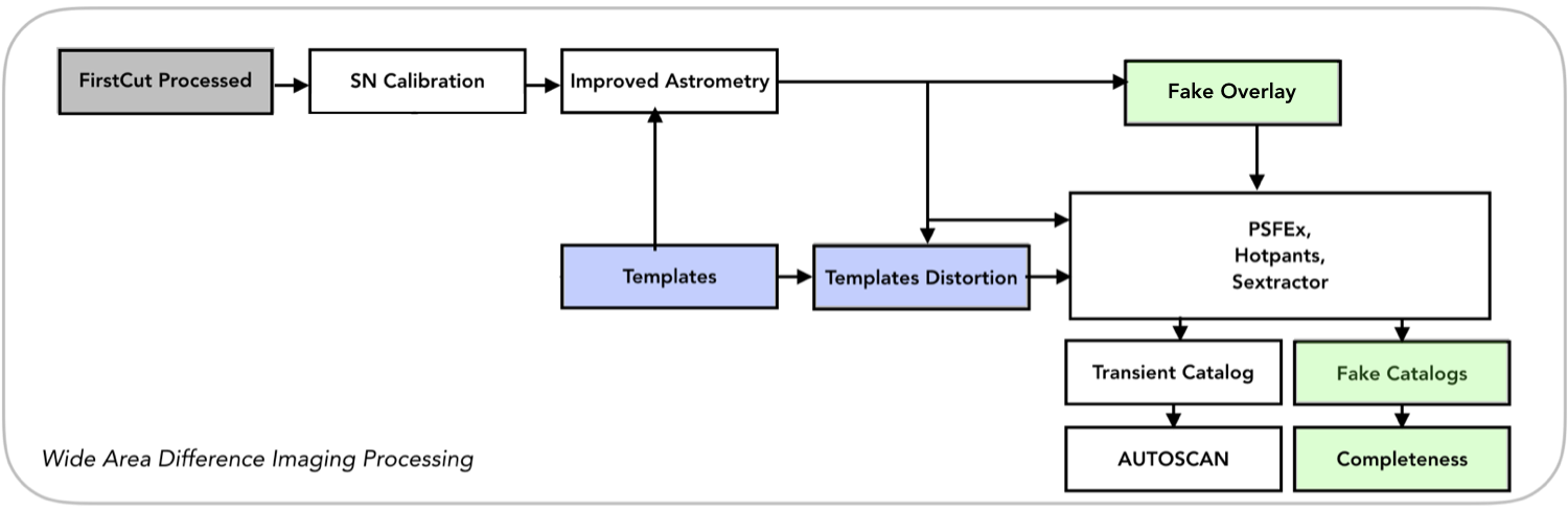
Figure 6: A diagram of the DiffImg processing used to detect transients in the wide area survey and in GW followup fields. Diagram based on Figure 7 of Morganson et al. (2018).

To identify GW EM counterpart candidates within
search images we use the aforementioned DiffImg software, originally developed for supernova searches in DES. Figure 6 illustrates the workflow. Using a feature of SCAMP, we calculate a joint astrometric solution on both the search and template image(s) using the 2MASS (O1 and O2 seasons) or GAIA-DR2 (O3) catalog. We perform the image subtraction via the HOTPANTS package (Becker, 2015). In our case, we perform a separate subtraction between the search image and each template, and then combine the difference images, rather than do a single subtraction on one combined template. While this approach is clearly slower than doing a single subtraction, it avoids potentially large PSF variations that could arise when combining templates taken in potentially very different observing conditions.

6.2.1 Template preparation

The DiffImg software, also sometimes known as the DiffImg “pipeline”, can accept as templates images that only partially overlap with search images, images that may have a relative rotation with respect to the search images, and images from DECam that were not taken on DES time (we only use such images if they have been publicly released). These are our main modifications of the pipeline relative to the DES supernova use case, where the search and template images are always exactly aligned (within telescope pointing errors) with one of a small set of fixed pointings that comprise the supernova survey area. After obtaining template images we apply the SE process to them as described in 6.1, so they are ready in the case of a LIGO event trigger. If the counterpart lies outside the DES footprint and no overlapping template image exists, template images of the appropriate area of the sky must be taken at a later time, after we expect any counterpart to have faded.

6.2.2 Fake injection

During the DiffImg run we inject fake point sources (generated ahead of time) into the search image in each band in random locations away from masked regions. These fakes can either vary in magnitude with time, or be fixed (typically at 20 in that case). Fakes are used for four purposes: to measure the “completeness depth”, or the depth at which we recover a specified fraction (typically 80%) of fakes in all of our search images (completeness depth thus reflects the variation in observing conditions); to monitor the single image detection efficiency; to monitor the multiple epoch detection efficiency; to characterize DiffImg for modeling in a catalog-level MC simulation.

To check our understanding of the efficiency measured with fakes we compare the measured efficiency to a prediction using a simulation from the Supernova Analysis software package, SNANA (Kessler et al., 2009, 2019), that analytically computes light curves without using the detection images, but by using the observed conditions and key properties of the images derived by measuring the fakes. This allows us to determine how well our sample selection criteria recover objects with known light curves. During O1 we measured a fake detection completeness of 80% or better down to magnitudes of 22.7 (21.8) in $i$ ($z$) band for 90-second exposures in good observing conditions (Soares-Santos et al., 2016).

6.2.3 Candidate identification

DiffImg identifies candidate objects by running
SExtractor on the difference images. Objects detected are filtered through a set of selection criteria listed in Table 1. Since the combined difference image includes correlated search image pixels summed over each template, the standard SExtractor flux uncertainties are not valid. We developed a special algorithm to properly account for correlations when determining the flux uncertainties. Surviving objects are referred to as “detections”. These detections then filter through a machine learning code, autoScan(Goldstein et al., 2015), which takes as input the template, search, and difference images and considers such items as 1) the ratio of PSF flux to aperture flux on the template image, 2) the magnitude difference between the detection and the nearest catalog source, and 3) the SExtractor-measured SPREAD_MODEL of the detection. autoScan returns a number between 0, an obvious artifact, and 1, a high-quality detection.

S/N $>3.5$

Object is PSF-like based on SPREAD MODEL

SExtractor A_IMAGE $<1.5\times$ PSF

In a $35\times 35$ box, $<200$ pixels with flux $<-2\sigma$ below $0$

In a $35\times 35$ box, $<20$ pixels with flux $<-4\sigma$ below $0$

In a $35\times 35$ box, $<2$ pixels with flux $<-6\sigma$ below $0$

Not within a mag-dependent radius of a veto catalog object

If coadded, CR rejection via consistency of detected object in each exposure

Table 1: Quality requirements for SExtractor objects detected in search images. From Table 3 of Kessler et al. 2015.

7 Postprocessing

The outputs of DiffImg are the inputs to our post-processing pipeline, illustrated in Fig. 7, which matches detections of the same objects across different exposures and applies quality assurance requirements. It also analyzes fakes injected into the images to assess the performance of DiffImg. This is in preparation for the final sample selection step.

Post-processing takes as input the collection of “raw” candidates from DiffImg, defined as when two or more detections have measured positions matching to within 1 arcsec. The two detections can be in the same band or different bands, or on the same night or different nights. All raw candidates are saved, which includes moving objects such as asteroids. Requiring detections on separate nights, or with a minimum time separation on the same night, helps to reject moving objects. In O1 and O2, we always took images in $i$ and/or $z$ bands in the initial search.

At this point, we also apply a minimum machine learning score requirement, typically 0.7, based on the autoScan score obtained during DiffImg. It is a choice to apply the autoScan requirement in post-processing rather than earlier in the process as it facilitates other detection completeness studies with looser requirements.

“Science candidates” are those raw candidates that pass the machine learning score requirement. For each science candidate we perform forced PSF photometry at the positions of the science candidates in all difference images that cover the location. Forced photometry provides flux measurements in all observations, regardless of the S/N.

There exists a “surface brightness anomaly” described in both Kessler et al. (2015) and Doctor et al. (2017) which degrades DiffImg search efficiency near large galaxies. The latter reports two effects: 1) excess missed detections of point sources in areas of high surface brightness as seen in large galaxies and 2) excess flux scatter in these same areas, which affects the selection of objects in analysis. Strategies to mitigate the effects remain an active area of research.

At this stage the science candidates still contain backgrounds, the leading examples of which are supernovae, asteroids, and M dwarf flare stars. We now impose additional selection criteria on the science candidates aimed at exploiting difference between kilonovae and these backgrounds. Below, we give some example criteria:

1. Supernovae: supernovae evolve more slowly than kilonovae or plausible BH counterparts. Example criteria to reject them: $\geq 3\sigma$ decline in both $i$ and $z$ fluxes from the first epoch to the second, and $\geq 2\sigma$ flux measurement in both $i$ and $z$ bands in the second epoch. In the case of a single-band search one can make similar flux requirements in the single band, and add additional requirements such as no increase in the candidate’s flux in any observation more than 48 hours after the GW event.

2. Asteroids: asteroids move on spatially relevant scales on timescales of minutes. Requiring detections separated in time by a sufficient amount, typically 30-60 minutes, eliminates these fast-moving objects. Slow moving asteroids are rare and faint.

3. M dwarf flare stars: While M stars are red, their flares are very blue, essentially 10,000K blackbodies. Example criterion for rejection: $\geq 3\sigma$ decline in $z$-band flux between epochs.

Several other types of objects can mimic a KN signal, as discussed in Cowperthwaite and Berger (2015), though they generally have rates two orders of magnitude or lower below the expected SN Ia rates.

All science candidates undergo a host matching process which identifies nearby galaxies and ranks them by probability of being the candidate’s host galaxy. This matching, implemented only for the latter portion of O2, uses a galaxy catalog consisting of data from the SDSS DR13 (Albareti et al., 2017), DES Y3Q2 (Abbott et al., 2018), and 2MASS photoz (Bilicki et al., 2014) catalogs.

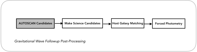
Figure 7: A diagram showing the postprocessing steps. Here the autoScan candidates refer to DiffImg detections or “raw” candidates, prior to the application of the tighter autoScan requirement. The host galaxy matching runs before forced photometry, but is not required. After forced photometry we can apply additional selection criteria as described in section 7.

8 Grid processing

In order to meet the turnaround time requirements we must make extensive use of grid resources. A typical observing night will generate between 100 and 200 new images, depending on the specifics of the observing plan and weather conditions. A typical SE processing job will take around three hours to complete, with DiffImg jobs running on a single CCD taking around one hour. Therefore one night’s worth of images requires between 6,000 and 12,000 CPU hours for the DiffImg stage, and between 300 and 600 additional hours for the SE processing stage. There could be some additional resources required if there are any template images with incomplete SE processing. Our program can effectively use resources at Fermilab and a wide variety of sites on the Open Science Grid, and can augment these capabilities by running on commercial clouds if needed. We use a job submission system (Jobsub; Box 2014) that sends GlideinWMS pilot jobs (Sfiligoi et al., 2009) to OSG sites. These pilots are shared among many Fermilab experiments, so due to the combined workload pressure from several experiments rather than just one, there are essentially always pilot jobs running that our workflow can use. We thus largely avoid a long ramp-up time often seen in pilot-based job submissions from a single experiment.

For a typical observing cadence we expect a new image to be available for processing every three to four minutes. As soon as each new image comes in during followup observations, we run a script that calculates which DECam images overlap with the new image and can be used as templates for DiffImg processing, checks whether SE processing is complete for that image, and then prepares a multi-stage HTCondor Directed Acyclic Graph that includes SE processing for new image and any incomplete templates in the first stage, with the DiffImg processing of the search image in the second stage. In the first stage there is one SE job per search, and in the DiffImg stage there is one job per CCD, for a total of 60 per search image, which run in parallel. The script also prepares a small custom tarball containing the exposure-specific DiffImg pipeline scripts and information about what template images overlaps with the search image. The script finishes by copying the tarball to Fermilab dCache (Fuhrmann and Gülzow, 2006) for use in the corresponding grid jobs, which are then immediately submitted. We distribute our main software stack to worker nodes via the CernVM File System (Blomer et al., 2011) mechanism.

9 Results from O1 and O2

During the first two LIGO observing seasons, we searched for an optical counterpart to a total of four BBH events, two each in O1 and O2, and one BNS event. During O1 we performed two analyses of GW150914 (Soares-Santos et al., 2016; Annis et al., 2016), and one of GW151226 (Cowperthwaite et al., 2016). During O2 we also followed up GW170104 and GW170814 (Doctor et al., 2019), covering 13.6% and 84% of the final LIGO 90% probability regions, respectively. We also performed followup observations of GW170817 (Abbott et al., 2017a), the first confirmed BNS event from LIGO that ushered in the multi-messenger astronomy era (Abbott et al., 2017b). Our analysis (Soares-Santos et al., 2017) resulted in one of several independent discoveries an optical counterpart near the galaxy NGC4993 11.4h post-merger in $i$ and $z$ bands. Our team also performed a GW170817 light curve analysis and made a comparison to KN models in Cowperthwaite et al. (2017). We also studied the GW170817 host galaxy, NGC 4993, and its environment in order to understand more about the formation of the GW source (Palmese et al., 2017). The fact that our pipeline detected the counterpart, and based on its initial magnitude could have detected a similar KN out to 425 Mpc, gives us confidence that we can detect future KNe past the expected LIGO sensitivity ranges in O3 and O4.

10 Future directions

We have used the system described in this paper to follow up LIGO sources from their observing runs O1 and O2. Our infrastructure is also well-suited to several other time-domain programs, including optical followup of high-energy neutrino events from the IceCube detector. IceCube can localize a neutrino event with a median angular resolution of $\leq 1.0$ sq. deg. on the sky, an area contained in a single DECam pointing. This program also aims to rapidly produce candidates for spectroscopic followup by other telescopes and is largely based on the pipeline developed here. The program released results in Morgan et al. (2019).

LIGO & Virgo continue to upgrade their laser interferometers. The full O3 run is expected to produce up to $~{}8$ merger events including neutron stars and dozens of binary black hole events. The expected rates are large enough to improve constraints on $H_{0}$, our primary science goal. These rates also present new challenges for the system described here, and we have implemented several pipeline upgrades for O3. For example we have expanded the available computing resources by running the DiffImg pipeline on commercial cloud resources. As part of the Fermilab HEPCloud project (Holzman et al., 2017) we ran DiffImg processing on Amazon EC2 resources. All tests passed. We are also adding the ability to incorporate non-DECam template images to increase our available sky coverage. Thirdly, we have modified the single-epoch processing steps so that they run on a CCD-by-CCD basis, allowing a single job per CCD to perform both single-epoch processing and image differencing. This change leads to fewer jobs overall and reduce the overhead associated with multiple jobs and eliminate the fact that in the O1/O2 system, image differencing would not proceed on any CCD until SE processing was complete on the entire image. In O3, each CCD can be proceed completely independently, reducing the time to science candidates by as much as a factor of five. Since astrometry is more difficult on a single CCD, we are using the GAIA-DR2 catalog (Gaia Collaboration et al., 2018) for astrometric calibration in O3.

11 Summary

The results from O1 and O2 demonstrate that our infrastructure can quickly get on sky following a ToO trigger, rapidly process new images, and carry out image differencing analysis in a timely manner. The infrastructure is not limited to GW event follow-up, however. It is trivial to apply the same techniques to a wide variety of astrophysical transient searches, including searches for Trans-Neptunian Objects, the hypothetical Planet Nine, and optical signatures from high-energy neutrino events detected by the IceCube experiment.

The DESGW program is a partnership between the Dark Energy Survey and members of the astronomy community. It is designed to search for electromagnetic counterparts to GW events, such as those expected from the merger of two neutron stars. DESGW is sensitive to BNS mergers out to approximately 400 Mpc. 2015 and early 2016 saw a successful first observing season with optical followup of two LVC triggers. The DESGW program was the most complete in terms of area covered and limiting magnitude of all EM counterpart followup programs that studied GW150914. The program completed a series of improvements to the computing infrastructure for followup observation preparation and to the imaging pipeline itself between the first two LIGO observing seasons. Season two started in November 2016, and saw followup of an additional two BBH events and an independent discovery of the EM counterpart to the first LIGO BNS merger. The infrastructure also performs well in a variety of time-domain astronomy programs. DESGW has excellent potential for discovering additional EM counterparts to future GW events, and is eagerly awaiting additional LIGO-Virgo triggers during the third observing season.

References

- Abbott et al. (2016a) Abbott, B.P., Abbott, R., Abbott, T.D., et al., 2016a. GW151226: Observation of Gravitational Waves from a 22-Solar-Mass Binary Black Hole Coalescence. Phys. Rev. Lett. 116, 241103. doi:10.1103/PhysRevLett.116.241103, arXiv:1606.04855.
- Abbott et al. (2016b) Abbott, B.P., Abbott, R., Abbott, T.D., et al., 2016b. Observation of Gravitational Waves from a Binary Black Hole Merger. Phys. Rev. Lett. 116, 061102. doi:10.1103/PhysRevLett.116.061102, arXiv:1602.03837.
- Abbott et al. (2017a) Abbott, B.P., Abbott, R., Abbott, T.D., et al., 2017a. GW170817: Observation of Gravitational Waves from a Binary Neutron Star Inspiral. Phys. Rev. Lett. 119, 161101. doi:10.1103/PhysRevLett.119.161101, arXiv:1710.05832.
- Abbott et al. (2017b) Abbott, B.P., Abbott, R., et al., 2017b. Multi-messenger Observations of a Binary Neutron Star Merger. Astrophys. J. 848, L12. doi:10.3847/2041-8213/aa91c9, arXiv:1710.05833.
- Abbott et al. (2018) Abbott, T.M.C., Abdalla, F.B., Allam, S., et al., 2018. The dark energy survey: Data release 1. Astrophys. J. Suppl. Ser. 239, 18. doi:10.3847/1538-4365/aae9f0.
- Albareti et al. (2017) Albareti, F.D., Allende Prieto, C., Almeida, A., et al., 2017. The 13th Data Release of the Sloan Digital Sky Survey: First Spectroscopic Data from the SDSS-IV Survey Mapping Nearby Galaxies at Apache Point Observatory. ApJs 233, 25. doi:10.3847/1538-4365/aa8992, arXiv:1608.02013.
- Annis et al. (2016) Annis, J., Soares-Santos, M., Berger, E., et al., 2016. A Dark Energy Camera Search for Missing Supergiants in the LMC after the Advanced LIGO Gravitational-wave Event GW150914. Astrophys. J. 823, L34. doi:10.3847/2041-8205/823/2/L34, arXiv:1602.04199.
- Barnes and Kasen (2013) Barnes, J., Kasen, D., 2013. Effect of a High Opacity on the Light Curves of Radioactively Powered Transients from Compact Object Mergers. Astrophys. J. 775, 18. doi:10.1088/0004-637X/775/1/18, arXiv:1303.5787.
- Barnes et al. (2016) Barnes, J., Kasen, D., Wu, M.R., Martínez-Pinedo, G., 2016. Radioactivity and Thermalization in the Ejecta of Compact Object Mergers and Their Impact on Kilonova Light Curves. Astrophys. J. 829, 110. doi:10.3847/0004-637X/829/2/110, arXiv:1605.07218.
- Becker (2015) Becker, A., 2015. HOTPANTS: High Order Transform of PSF ANd Template Subtraction. Astrophysics Source Code Library. URL: https://github.com/acbecker/hotpants, arXiv:1504.004.
- Berger (2014) Berger, E., 2014. Short-Duration Gamma-Ray Bursts. Annu. Rev. Astron. Astrophys. 52, 43–105. doi:10.1146/annurev-astro-081913-035926, arXiv:1311.2603.
- Bernstein et al. (2018) Bernstein, G.M., Abbott, T.M.C., Armstrong, R., et al., 2018. Photometric Characterization of the Dark Energy Camera. Publ. Astron. Soc. Pac. 130, 054501. doi:10.1088/1538-3873/aaa753, arXiv:1710.10943.
- Bertin (2006) Bertin, E., 2006. Automatic Astrometric and Photometric Calibration with SCAMP. volume 351 of Astron. Soc. Pac. Conf. Ser. p. 112.
- Bertin (2011) Bertin, E., 2011. Automated Morphometry with SExtractor and PSFEx, in: Evans, I.N., Accomazzi, A., Mink, D.J., Rots, A.H. (Eds.), Astronomical Data Analysis Software and Systems XX, p. 435.
- Bilicki et al. (2014) Bilicki, M., Jarrett, T.H., Peacock, J.A., et al., 2014. Two Micron All Sky Survey Photometric Redshift Catalog: A Comprehensive Three-dimensional Census of the Whole Sky. Astrophys. J. Suppl. Ser. 210, 9. doi:10.1088/0067-0049/210/1/9, arXiv:1311.5246.
- Blomer et al. (2011) Blomer, J., Aguado-Sánchez, C., Buncic, P., Harutyunyan, A., 2011. Distributing LHC application software and conditions databases using the CernVM file system, in: J. Phys.: Conf. Ser., p. 042003. doi:10.1088/1742-6596/331/4/042003.
- Box (2014) Box, D., 2014. FIFE-Jobsub: a grid submission system for intensity frontier experiments at Fermilab. J. Phys.: Conf. Ser. 513, 032010. doi:10.1088/1742-6596/513/3/032010.
- Bulla (2019) Bulla, M., 2019. POSSIS: predicting spectra, light curves and polarization for multi-dimensional models of supernovae and kilonovae. arXiv e-prints , arXiv:1906.04205arXiv:1906.04205.
- Chen et al. (2018) Chen, H.Y., Fishbach, M., Holz, D.E., 2018. A two per cent Hubble constant measurement from standard sirens within five years. Nature 562, 545–547. doi:10.1038/s41586-018-0606-0, arXiv:1712.06531.
- Cowperthwaite and Berger (2015) Cowperthwaite, P.S., Berger, E., 2015. A Comprehensive Study of Detectability and Contamination in Deep Rapid Optical Searches for Gravitational Wave Counterparts. Astrophys. J. 814, 25. doi:10.1088/0004-637X/814/1/25, arXiv:1503.07869.
- Cowperthwaite et al. (2016) Cowperthwaite, P.S., Berger, E., Soares-Santos, M., et al., 2016. A DECam Search for an Optical Counterpart to the LIGO Gravitational-wave Event GW151226. Astrophys. J. 826, L29. doi:10.3847/2041-8205/826/2/L29, arXiv:1606.04538.
- Cowperthwaite et al. (2017) Cowperthwaite, P.S., Berger, E., Villar, V.A., et al., 2017. The Electromagnetic Counterpart of the Binary Neutron Star Merger LIGO/Virgo GW170817. II. UV, Optical, and Near-infrared Light Curves and Comparison to Kilonova Models. Astrophys. J. 848, L17. doi:10.3847/2041-8213/aa8fc7, arXiv:1710.05840.
- Del Pozzo (2012) Del Pozzo, W., 2012. Inference of cosmological parameters from gravitational waves: Applications to second generation interferometers. Phys. Rev. D 86, 043011. doi:10.1103/PhysRevD.86.043011, arXiv:1108.1317.
- Doctor et al. (2017) Doctor, Z., Kessler, R., Chen, H.Y., et al., 2017. A Search for Kilonovae in the Dark Energy Survey. Astrophys. J. 837, 57. doi:10.3847/1538-4357/aa5d09, arXiv:1611.08052.
- Doctor et al. (2019) Doctor, Z., Kessler, R., Herner, K., et al., 2019. A Search for Optical Emission from Binary Black Hole Merger GW170814 with the Dark Energy Camera. Astrophys. J. Lett. 873, L24. doi:10.3847/2041-8213/ab08a3, arXiv:1812.01579.
- Duque et al. (2019) Duque, R., Daigne, F., Mochkovitch, R., 2019. Predictions for radio afterglows of binary neutron star mergers: a population study for O3 and beyond. arXiv e-prints , arXiv:1905.04495arXiv:1905.04495.
- Fahlman and Fernández (2018) Fahlman, S., Fernández, R., 2018. Hypermassive Neutron Star Disk Outflows and Blue Kilonovae. Astrophys. J. Lett. 869, L3. doi:10.3847/2041-8213/aaf1ab, arXiv:1811.08906.
- Flaugher et al. (2015) Flaugher, B., Diehl, H.T., Honscheid, K., et al., 2015. The Dark Energy Camera. Astron. J. 150, 150. doi:10.1088/0004-6256/150/5/150, arXiv:1504.02900.
- Fuhrmann and Gülzow (2006) Fuhrmann, P., Gülzow, V., 2006. dcache, storage system for the future, in: Nagel, W.E., Walter, W.V., Lehner, W. (Eds.), Euro-Par 2006 Parallel Processing, Springer Berlin Heidelberg, Berlin, Heidelberg. pp. 1106–1113.
- Gaertig et al. (2011) Gaertig, E., Glampedakis, K., Kokkotas, K.D., Zink, B., 2011. f-Mode Instability in Relativistic Neutron Stars. Phys. Rev. Lett. 107, 101102. doi:10.1103/PhysRevLett.107.101102, arXiv:1106.5512.
- Gaia Collaboration et al. (2018) Gaia Collaboration, Brown, A.G.A., Vallenari, A., Prusti, T., et al., 2018. Gaia Data Release 2. Summary of the contents and survey properties. Astron. & Astrophys. 616, A1. doi:10.1051/0004-6361/201833051, arXiv:1804.09365.
- Gaia Collaboration et al. (2016) Gaia Collaboration, Prusti, T., de Bruijne, J.H.J., Brown, A.G.A., et al., 2016. The Gaia mission. Astron. & Astrophys. 595, A1. doi:10.1051/0004-6361/201629272, arXiv:1609.04153.
- Goldstein et al. (2015) Goldstein, D.A., D’Andrea, C.B., Fischer, J.A., et al., 2015. Automated Transient Identification in the Dark Energy Survey. Astron. J. 150, 82. doi:10.1088/0004-6256/150/3/82, arXiv:1504.02936.
- Gompertz et al. (2018) Gompertz, B.P., Levan, A.J., Tanvir, N.R., et al., 2018. The Diversity of Kilonova Emission in Short Gamma-Ray Bursts. Astrophys. J. 860, 62. doi:10.3847/1538-4357/aac206, arXiv:1710.05442.
- Górski et al. (2005) Górski, K.M., Hivon, E., Banday, A.J., et al., 2005. HEALPix: A Framework for High-Resolution Discretization and Fast Analysis of Data Distributed on the Sphere. Astrophys. J. 622, 759–771. doi:10.1086/427976, arXiv:astro-ph/0409513.
- Gottlieb et al. (2018) Gottlieb, O., Nakar, E., Piran, T., 2018. The cocoon emission - an electromagnetic counterpart to gravitational waves from neutron star mergers. Mon. Not. R. Astron. Soc. 473, 576–584. doi:10.1093/mnras/stx2357, arXiv:1705.10797.
- Greisen and Calabretta (2002) Greisen, E.W., Calabretta, M.R., 2002. Representations of world coordinates in FITS. Astron. & Astrophys. 395, 1061–1075. doi:10.1051/0004-6361:20021326, arXiv:astro-ph/0207407.
- Grossman et al. (2014) Grossman, D., Korobkin, O., Rosswog, S., Piran, T., 2014. The long-term evolution of neutron star merger remnants - II. Radioactively powered transients. Mon. Not. R. Astron. Soc. 439, 757–770. doi:10.1093/mnras/stt2503, arXiv:1307.2943.
- Holz and Hughes (2005) Holz, D.E., Hughes, S.A., 2005. Using gravitational-wave standard sirens. Astrophys. J. 629, 15. URL: http://stacks.iop.org/0004-637X/629/i=1/a=15.
- Holzman et al. (2017) Holzman, B., Bauerdick, L.A.T., Bockelman, B., et al., 2017. Hepcloud, a new paradigm for HEP facilities: CMS Amazon Web Services investigation. Comput. and Softw. for Big Sci. 1, 1. URL: https://doi.org/10.1007/s41781-017-0001-9, doi:10.1007/s41781-017-0001-9.
- Kessler et al. (2009) Kessler, R., Bernstein, J.P., Cinabro, D., et al., 2009. SNANA: A Public Software Package for Supernova Analysis. Publ. Astron. Soc. Pac. 121, 1028. doi:10.1086/605984, arXiv:0908.4280.
- Kessler et al. (2019) Kessler, R., Brout, D., D’Andrea, C.B., et al., 2019. First cosmology results using Type Ia supernova from the Dark Energy Survey: simulations to correct supernova distance biases. Mon. Not. R. Astron. Soc. 485, 1171–1187. doi:10.1093/mnras/stz463, arXiv:1811.02379.
- Kessler et al. (2015) Kessler, R., Marriner, J., Childress, M., et al., 2015. The Difference Imaging Pipeline for the Transient Search in the Dark Energy Survey. Astron. J. 150, 172. doi:10.1088/0004-6256/150/6/172, arXiv:1507.05137.
- Krisciunas and Schaefer (1991) Krisciunas, K., Schaefer, B.E., 1991. A model of the brightness of moonlight. Publ. Astron. Soc. Pac. 103, 1033–1039. doi:10.1086/132921.
- Lindegren et al. (2018) Lindegren, L., Hernández, J., Bombrun, A., et al., 2018. Gaia Data Release 2. The astrometric solution. Astron. & Astrophys. 616, A2. doi:10.1051/0004-6361/201832727, arXiv:1804.09366.
- MacLeod and Hogan (2008) MacLeod, C.L., Hogan, C.J., 2008. Precision of Hubble constant derived using black hole binary absolute distances and statistical redshift information. Phys. Rev. D 77, 043512. doi:10.1103/PhysRevD.77.043512, arXiv:0712.0618.
- Metzger (2017) Metzger, B.D., 2017. Kilonovae. Living Reviews in Relativity 20, 3. doi:10.1007/s41114-017-0006-z, arXiv:1610.09381.
- Metzger and Berger (2012) Metzger, B.D., Berger, E., 2012. What is the Most Promising Electromagnetic Counterpart of a Neutron Star Binary Merger? Astrophys. J. 746, 48. doi:10.1088/0004-637X/746/1/48, arXiv:1108.6056.
- Metzger et al. (2010) Metzger, B.D., Martínez-Pinedo, G., Darbha, S., et al., 2010. Electromagnetic counterparts of compact object mergers powered by the radioactive decay of r-process nuclei. Mon. Not. R. Astron. Soc. 406, 2650–2662. doi:10.1111/j.1365-2966.2010.16864.x, arXiv:1001.5029.
- Morgan et al. (2019) Morgan, R., Bechtol, K., Kessler, R., et al., 2019. A DECam Search for Explosive Optical Transients Associated with IceCube Neutrino Alerts. Astrophys. J. 883, 125. doi:10.3847/1538-4357/ab3a45.
- Morganson et al. (2018) Morganson, E., Gruendl, R.A., Menanteau, F., et al., 2018. The Dark Energy Survey Image Processing Pipeline. Publ. Astron. Soc. Pac. 130, 074501. doi:10.1088/1538-3873/aab4ef, arXiv:1801.03177.
- Nair et al. (2018) Nair, R., Bose, S., Saini, T.D., 2018. Measuring the Hubble constant: Gravitational wave observations meet galaxy clustering. Phys. Rev. D 98, 023502. doi:10.1103/PhysRevD.98.023502, arXiv:1804.06085.
- Nissanke et al. (2013) Nissanke, S., Holz, D.E., Dalal, N., et al., 2013. Determining the Hubble constant from gravitational wave observations of merging compact binaries. arXiv e-prints , arXiv:1307.2638arXiv:1307.2638.
- Nissanke et al. (2010) Nissanke, S., Holz, D.E., Hughes, S.A., et al., 2010. Exploring Short Gamma-ray Bursts as Gravitational-wave Standard Sirens. Astrophys. J. 725, 496–514. doi:10.1088/0004-637X/725/1/496, arXiv:0904.1017.
- Palmese et al. (2017) Palmese, A., Hartley, W., Tarsitano, F., et al., 2017. Evidence for Dynamically Driven Formation of the GW170817 Neutron Star Binary in NGC 4993. Astrophys. J. 849, L34. doi:10.3847/2041-8213/aa9660, arXiv:1710.06748.
- Palmese and Kim (2020) Palmese, A., Kim, A.G., 2020. Probing gravity and growth of structure with gravitational waves and galaxies’ peculiar velocity. arXiv e-prints , arXiv:2005.04325arXiv:2005.04325.
- Pan et al. (2017) Pan, Y.C., Foley, R.J., Smith, M., et al. (The DES Collaboration), 2017. DES15E2mlf: a spectroscopically confirmed superluminous supernova that exploded 3.5 Gyr after the big bang. Mon. Not. R. Astron. Soc. 470, 4241–4250. doi:10.1093/mnras/stx1467, arXiv:1707.06649.
- Paschalidis and Ruiz (2019) Paschalidis, V., Ruiz, M., 2019. Are fast radio bursts the most likely electromagnetic counterpart of neutron star mergers resulting in prompt collapse? Phys. Rev. D 100, 043001. URL: https://link.aps.org/doi/10.1103/PhysRevD.100.043001, doi:10.1103/PhysRevD.100.043001.
- Pordes et al. (2007) Pordes, R., Petravick, D., Kramer, B., et al., 2007. The open science grid. J. Phys.: Conf. Ser. 78, 012057. URL: https://doi.org/10.1088%2F1742-6596%2F78%2F1%2F012057, doi:10.1088/1742-6596/78/1/012057.
- Pursiainen et al. (2018) Pursiainen, M., Childress, M., Smith, M., et al. (The DES Collaboration), 2018. Rapidly evolving transients in the Dark Energy Survey. Mon. Not. R. Astron. Soc. 481, 894–917. doi:10.1093/mnras/sty2309.
- Radice et al. (2018) Radice, D., Perego, A., Hotokezaka, K., et al., 2018. Binary Neutron Star Mergers: Mass Ejection, Electromagnetic Counterparts, and Nucleosynthesis. Astrophys. J. 869, 130. doi:10.3847/1538-4357/aaf054, arXiv:1809.11161.
- Riess et al. (2019) Riess, A.G., Casertano, S., Yuan, W., et al., 2019. Large Magellanic Cloud Cepheid Standards Provide a 1% Foundation for the Determination of the Hubble Constant and Stronger Evidence for Physics beyond CDM. Astrophys. J. 876, 85. doi:10.3847/1538-4357/ab1422, arXiv:1903.07603.
- Rosswog et al. (2017) Rosswog, S., Feindt, U., Korobkin, O., et al., 2017. Detectability of compact binary merger macronovae. Class. and Quantum Gravity 34, 104001. doi:10.1088/1361-6382/aa68a9, arXiv:1611.09822.
- Schutz (1986) Schutz, B.F., 1986. Determining the Hubble constant from gravitational wave observations. Nature 323, 310. doi:10.1038/323310a0.
- Sfiligoi et al. (2009) Sfiligoi, I., Bradley, D.C., Holzman, B., et al., 2009. The pilot way to grid resources using glideinwms, in: Proceedings of the 2009 WRI World Congress on Computer Science and Information Engineering - Volume 02, IEEE Computer Society, Washington, DC, USA. pp. 428–432. URL: https://doi.org/10.1109/CSIE.2009.950, doi:10.1109/CSIE.2009.950.
- Singer et al. (2016) Singer, L.P., Chen, H.Y., Holz, D.E., et al., 2016. Supplement: “Going the Distance: Mapping Host Galaxies of LIGO and Virgo Sources in Three Dimensions Using Local Cosmography and Targeted Follow-up” (2016, ApJ, 829, L15). Astrophys. J. s 226, 10. doi:10.3847/0067-0049/226/1/10, arXiv:1605.04242.
- Skrutskie et al. (2006) Skrutskie, M.F., Cutri, R.M., Stiening, R., et al., 2006. The Two Micron All Sky Survey (2MASS). Astron. J. 131, 1163–1183. doi:10.1086/498708.
- Soares-Santos et al. (2017) Soares-Santos, M., Holz, D.E., Annis, J., et al., 2017. The Electromagnetic Counterpart of the Binary Neutron Star Merger LIGO/Virgo GW170817. I. Discovery of the Optical Counterpart Using the Dark Energy Camera. Astrophys. J. 848, L16. doi:10.3847/2041-8213/aa9059, arXiv:1710.05459.
- Soares-Santos et al. (2016) Soares-Santos, M., Kessler, R., Berger, E., et al., 2016. A Dark Energy Camera Search for an Optical Counterpart to the First Advanced LIGO Gravitational Wave Event GW150914. Astrophys. J. 823, L33. doi:10.3847/2041-8205/823/2/L33, arXiv:1602.04198.
- Soares-Santos & Palmese et al. (2019) Soares-Santos & Palmese, Hartley, W., et al., 2019. First measurement of the hubble constant from a dark standard siren using the dark energy survey galaxies and the LIGO/virgo binary–black-hole merger GW170814. Astrophys. J. 876, L7. URL: https://doi.org/10.3847%2F2041-8213%2Fab14f1, doi:10.3847/2041-8213/ab14f1.
- Tanaka and Hotokezaka (2013) Tanaka, M., Hotokezaka, K., 2013. Radiative Transfer Simulations of Neutron Star Merger Ejecta. Astrophys. J. 775, 113. doi:10.1088/0004-637X/775/2/113, arXiv:1306.3742.
- Tanaka et al. (2018) Tanaka, M., Kato, D., Gaigalas, G., et al., 2018. Properties of Kilonovae from Dynamical and Post-merger Ejecta of Neutron Star Mergers. Astrophys. J. 852, 109. doi:10.3847/1538-4357/aaa0cb, arXiv:1708.09101.
- Villar et al. (2017) Villar, V.A., Guillochon, J., Berger, E., et al., 2017. The Combined Ultraviolet, Optical, and Near-infrared Light Curves of the Kilonova Associated with the Binary Neutron Star Merger GW170817: Unified Data Set, Analytic Models, and Physical Implications. Astrophys. J. Lett. 851, L21. doi:10.3847/2041-8213/aa9c84, arXiv:1710.11576.
- Young (1994) Young, A.T., 1994. Air mass and refraction. Appl. Opt. 33, 1108–1110. doi:10.1364/AO.33.001108.
- Zacharias et al. (2004) Zacharias, N., Monet, D.G., Levine, S.E., et al., 2004. The Naval Observatory Merged Astrometric Dataset (NOMAD), in: American Astronomical Society Meeting Abstracts, p. 48.15.