Predictability limit of partially observed systems

Applications from finance to epidemiology and cyber-security require accurate forecasts of dynamic phenomena, which are often only partially observed. We demonstrate that a system’s predictability degrades as a function of temporal sampling, regardless of the adopted forecasting model. We quantify the loss of predictability due to sampling, and show that it cannot be recovered by using external signals. We validate the generality of our theoretical findings in real-world partially observed systems representing infectious disease outbreaks, online discussions, and software development projects. On a variety of prediction tasks—forecasting new infections, the popularity of topics in online discussions, or interest in cryptocurrency projects—predictability irrecoverably decays as a function of sampling, unveiling fundamental predictability limits in partially observed systems.

Introduction

Forecasting complex dynamic phenomena — from influenza outbreaks to public opinions, stock market, and cyberattacks — is central to many policy and national security applications  (?). Prediction is also the standard framework in evaluating models of complex systems learned from data  (?). Time series forecasting, which underpins popular models of dynamic phenomena, represents a process as a sequence of observations (discrete or continuous numbers of events) at regular time intervals. After learning parameters from past observations, the models can be used to predict future observations  (?). Forecasting models based on stochastic and self-exciting point processes, autoregressive and hidden Markov models, have been developed to predict crime  (?, ?), social unrest  (?), terrorism  (?), epidemics  (?), human mobility  (?), personal correspondence  (?), online activity  (?, ?), dynamics of ecological systems  (?, ?) and more  (?).

A fundamental challenge to modeling efforts is the fact that complex systems are seldom fully observed. For example, when estimating opinions in a social system, it is not practical nor feasible to interview every individual in the population; instead, polling is used to elicit responses from a representative sample of a population. When social media is used as a proxy of opinions, it is similarly impractical to collect all relevant posts; instead, a (pseudo-random) sample (e.g., the Twitter Decahose), is often used. Further biases can emerge when data is deliberately manipulated or deleted, e.g., to obfuscate or censor content or activity  (?). In short, the data used to learn predictive models of complex phenomena often represents a highly filtered and incomplete view.

How does data loss due to sampling affect the predictability of complex systems and the accuracy of models learned from the data? Statisticians have developed a number of approaches to compensate for data loss, including data imputation  (?) to fill in missing values and evaluating the representativeness of the sample  (?, ?). Few of these approaches apply to temporal data. To quantify the predictability of dynamic systems, researchers use measures such as autocorrelation and permutation entropy. The former measures similarity between a time series and its own time-lagged versions. Recently, permutation entropy was introduced as a model-free, nonlinear indicator of the complexity of data  (?, ?). Permutation entropy represents the complexity of a time series through statistics of its ordered sub-sequences, also known as motifs, and has been adopted to model predictability of ecological systems  (?, ?) and epidemic outbreaks  (?). However, the impact of sampling on these measures of predictability of complex systems is not known.

As the first step towards addressing this question, we model incomplete observation as a stochastic sampling process that selects events at random with some probability $p$ and drops the remaining events from observations of a system. This allows us to theoretically characterize how sampling decreases the autocorrelation of a time series. We then empirically show that sampling also reduces the predictability of a dynamic process according to both autocorrelation and permutation entropy. Moreover, the loss of predictability cannot be fully recovered from some external signal, even using data highly correlated with the original unsampled process. As a result, forecasts made by autoregressive models may be no better than predictions of simpler, less accurate models that assume independent events. We validate these findings with both synthetic and real-world data representing complex social and techno-social systems. Without any modeling assumptions on the data, we show how sampling systematically degrades the predictability of these systems.

Researchers increasingly predict complex systems and social network dynamics  (?, ?, ?, ?) to learn the principles of human and machine behavior  (?, ?). Practitioners and lawmakers alike often base their decisions on such insights  (?, ?), including for public health  (?, ?) and public policy  (?, ?, ?, ?). As some pointed out  (?, ?), however, caution should be used when drawing conclusions from incomplete data. Sampling, even random sampling, distorts the observed dynamics of a process, reducing its predictability. We formalize and quantify this common, yet understudied, source of bias in partially observed systems.

Results

Model

Consider a dynamic process generating events, for example, social media posts mentioning a particular topic, or newly infected individuals during an epidemic. We can represent the process as a time series of event counts, $X=[X_{1},X_{2},\ldots,X_{T}]$, each entry representing the number of observations of $X$ at time $t$. We refer to this time series as the ground truth signal.

Observers of this process may not see all events. Twitter, for example, makes only a small fraction ($\leq 10\%$) of messages posted on its platform programmatically available. Similarly, hospitals may delay reporting new cases of a disease or under-count them altogether when, for various reasons, people do not seek medical help after getting sick. We refer to the time series of observed events $Y=[Y_{1},Y_{2},\ldots,Y_{T}]$ as the observed signal. Intuitively, $Y$ represents a sample of events present in the ground truth signal $X$.

Figure 1: Sampling paradigm as a representation of a partially observed dynamic process. Here, $X$, the ground truth signal, represents the actual events, e.g., Twitter posts mentioning a particular topic; $Y$ represents the observed subset of events. The funnel illustrates the sampling process. The probability of an event being observed is $p$. The Binomial distribution $B(X,p)$ is used to model the observed signal $Y$.

We model partial observation as a stochastic sampling process, where each event has some probability to be observed, independent of other events. This allows us to formalize how the time series of the ground truth and the observed signals are related. Figure 1 illustrates this paradigm.

Definition 1.

We define sampling rate $p\in[0,1]$ as the percentage of events that are preserved by the observation process. Let $X$ and $Y$ be two time series related by

$$Y\sim B([X],p),$$

where $B([X],p)$ is a Binomial process with $[X]$ trials, each with success probability $p$.

The factors driving the system may also produce some external events that may help predict the observed system. For example, rising temperatures associated with climate change may help better forecast epidemics that are made more virulent by changes in climate. Similarly, news reports may be associated with increased social media posts on specific topics, since both are driven by world events. Temperatures and news reports may provide important signals for predicting future events.

Definition 2.

We define the external signal as the time series $S=S_{1},S_{2},\ldots,S_{T}$ that may provide information about the ground truth signal.

Quantifying the Loss of Predictability

Researchers have devised measures of predictability of complex systems. At the simplest level, autocorrelation captures how well a time series representing a complex system is correlated with its own time-lagged versions. This indicator of predictability is popular in finance  (?). In ecology and physics, permutation entropy is used to measure predictability  (?, ?). Permutation entropy (PE) captures the complexity of a time series through statistics of its ordered sub-sequences, or motifs (see Materials & Methods). The higher the permutation entropy, the more diverse the motifs, which in turn renders the time series less predictable. Permutation entropy was shown to be strongly related to Kolmogorov-Sinai (KS) entropy  (?), a theoretical measure quantifying the complexity of a dynamical system. KS is not easy to reliably estimate from data; however, for one dimensional time-series, KS and permutation entropy are known to be equivalent under a variety of conditions  (?). Using different forecasting models, Garland et al.  (?) demonstrated an empirical correlation between predictability of the models and permutation entropy  (?). Since then, PE has been used as a model-free indicator of predictability of infectious disease outbreaks  (?), human mobility  (?), ecological systems  (?), and anomaly detection in paleoclimate records  (?). Besides autocorrelation and PE, we also use prediction error as a measure of predictability  (?). However, since prediction error depends on the forecasting model, we explore it in detail only with synthetic data (SI, Synthetic Data Experiments).

We show that sampling reduces predictability of a signal, and the more data is filtered out, the less predictable the signal becomes. The loss of predictability cannot be recovered using an informative external signal, even if it is highly correlated with the original ground truth signal. We develop a framework for quantifying predictability loss due to sampling and validate it empirically using all measures of predictability.

Our main theoretical contribution is an analytical characterization of the covariance matrix of the observed signal $Y$ in terms of the ground truth signal $X$ and the sampling rate $p$ (cf., Materials & Methods, Theorem 1). Theorems and their proofs are presented in the SI. Based on this characterization, we derive two results stating the effects of sampling on the predictability of the observed signal $Y$:

Decay of autocorrelation of the observed signal.

The autocorrelation (defined as Pearson correlation between values of the signal at different times) of the observed signal $Y$ decays monotonically at lower sampling rates (Corollary 2, Materials & Methods).

Decay of covariance with the external signal.

The correlation between the observed and external signals degrades linearly at lower sampling rates (Corollary 3, Materials & Methods).

Specifically, to quantify the impact of sampling on the predictability of a signal, we first derive the autocorrelation of the observed signal as a function of the sampling rate $p$ (cf., Corollary 1, Materials & Methods). When $p=1$ (i.e., complete observation), we recover the autocorrelation of the ground truth signal $X$. At lower sampling rates, the autocorrelation decays as postulated above. In parallel, we demonstrate empirically that sampling degrades predictability as measured using permutation entropy.

A forecasting model may compensate for the loss of predictability by leveraging an informative external signal. For example, auto-regressive forecasting models allow for additional covariates to improve predictions  (?). However, according to our second result, predictability cannot be fully recovered with an external signal, even one that is highly correlated with the ground truth signal.

Empirical Results

We show that sampling irreversibly degrades the predictability of real-world complex systems, studying three phenomena: disease outbreaks, online discussions, and software collaborations. Sampling reduces predictability according to both autocorrelation and permutation entropy measures, and the observed decay of autocorrelation agrees with theoretical predictions.

Predictability cannot be fully recovered using an informative external signal. In addition to co-variance, we use mutual information (MI) to measure the shared information between the external and the observed signals  (?). Mutual information quantifies the reduction in uncertainty about one random variable due to the presence of another  (?), and like PE it captures the non-linearities in the data that covariance cannot measure. We empirically find that sampling reduces both the covariance and MI with the external signal.

Epidemics.

Scarpino & Petri  (?) used permutation entropy to show that predictability of disease outbreaks decreases over longer time periods, suggesting changes in the behavior of epidemics over time. Here, we show that the predictability of epidemics is also affected by how partially or fully observed the new infections are.

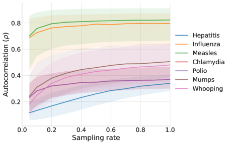
Figure 14: Theoretical and empirical Loss of autocorrelation in outbreaks due to sampling for all diseases. The plot depicts a decrease on the autocorrelation as drop-out rate increase. For each of the eight weekly, state-level diseases, we selected $100$ random points and calculated the entropy and autocorrelation for different drop-out rates over a one year window. The solid line represents the median, shaded region marks the interquartile range.

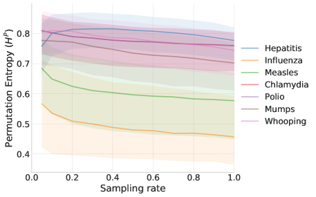
Figure 15: Loss of predictability due to sampling for all diseases. The plot shows and increase on the permutation entropy as drop-out rate increase. For each of the eight weekly, state-level diseases, we selected $100$ random points and calculated the entropy and autocorrelation for different drop-out rates over a one year window. The solid line represents the median, shaded region marks the interquartile range.

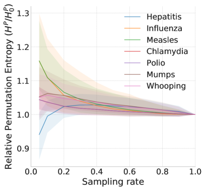
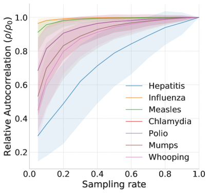
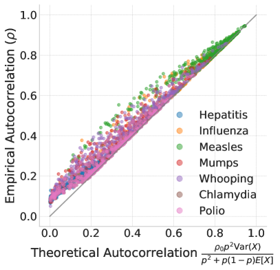
Figure 17: Loss of predictability of disease outbreaks due to sampling. The plots show a decrease in permutation entropy (top-left) and an increase in autocorrelation (top-right) of the outbreak time series for increasing sampling rates. For each of the eight diseases, we selected $100$ random two-year time windows and calculated the relative weighted permutation entropy and autocorrelation for different sampling rates over that window. The solid line represents the median ratio across all states between the original time series and the sampled one; shaded regions mark the inter-quartile ranges. The bottom plot supports our theoretical results by plotting Equation 3 against the empirical autocorrelation of the sampled time series at different sampling rates for each disease.

We study eight diseases (Chlamydia, Gonorrhea, Hepatitis A, Influenza, Measles, Mumps, Polio, and Whooping cough), representing each disease outbreak as a time series of the weekly number of reported infections in each US state. We find that at lower sampling rates, the permutation entropy (PE), over one-year moving windows (although the results are robust to longer windows, see SI Figure 17), of the times series increases (Figure 2 (top-left)) and the autocorrelation decreases (Figure 2 (top-right)). Given that each disease has a different base PE and autocorrelation coefficient (see SI, Figures 14 and 15 for the absolute values), we normalized the predictability measure of the sampled time series by the corresponding measure of the ground truth time series (i.e., with full information, corresponding to sampling rate $p=1$) to capture the relative change. The observed loss of autocorrelation for each disease outbreak at different sampling rates (Figure 2 (bottom)) agrees well with the theoretical predictions derived by Equation 3. Our findings suggest that observing only a subset of the new infections distorts the observed dynamics of the disease, making the outbreak less predictable.

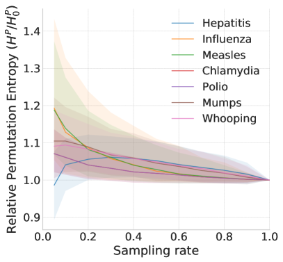
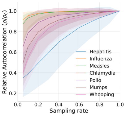
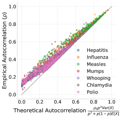
Figure 2: Loss of predictability of disease outbreaks due to sampling. The plots show a decrease in permutation entropy (top-left) and an increase in autocorrelation (top-right) of the outbreak time series for increasing sampling rates. For each of the eight diseases, we selected $100$ random one-year time windows and calculated the relative weighted permutation entropy and autocorrelation for different sampling rates over that window. The solid line represents the median ratio across all states between the original time series and the sampled one; shaded regions mark the inter-quartile ranges. The bottom plot supports our theoretical results by plotting Equation 3 against the empirical autocorrelation of the sampled time series at different sampling rates for each disease.

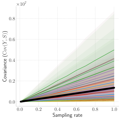
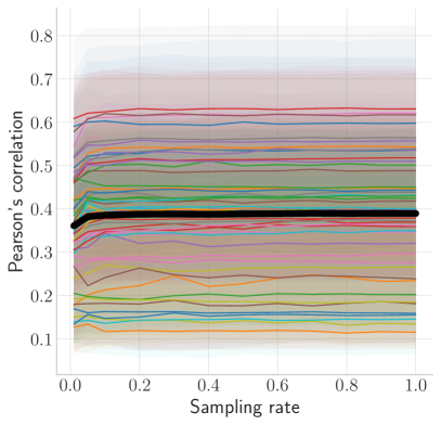
Figure 3: Decay of covariance between ground truth and external signals. For each state, we selected $100$ random one-year time windows and calculated the median covariance (left) and Pearson’s correlation (right) between Google Flu trends and the influenza activity at different sampling rates. Shaded regions mark the inter-quartile ranges for each state; the solid line represents the average coefficient across all states.

Next, we use influenza data to validate Corollary 3, which states that an external signal becomes less informative (i.e., has lower covariance) about the ground truth data at lower sampling rates. As an external signal $S$, we use state-level Google Flu trends  (?), which estimate influenza activity based on search queries. Figure 3 (left) shows a linear growth of covariance for each state’s influenza time series with increasing sampling rate. However, as depicted on the right plot, there is no observed loss of correlation for lower sampling rates. This is due to the large variance relative to the mean exhibited by influenza activity. From Theorem 1, we have that the standard deviation of the observed signal $Y$ is

$$\sigma_{Y}=\sqrt{p^{2}\mathrm{Var}(X)+p(1-p)\mathbb{E}[X]}\approx p\;\sigma_{X}$$

when $\mathrm{Var}(X)\gg\mathbb{E}[X]$. Then, it follows from Corollary 3 and the definition of Pearson’s correlation $\rho$, that

$$\rho_{Y,S}=\frac{\mathrm{Cov}(Y,S)}{\sigma_{Y}\sigma_{S}}\approx\frac{p\;\mathrm{Cov}(X,S)}{p\;\sigma_{X}\sigma_{S}}=\rho_{X,S}.$$

Thus, the linear decrease of covariance is offset by a linear decrease of the standard deviation. However, this is not always the case, as we later show with the cryptocurrency popularity scenario.

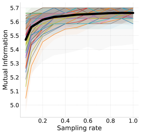
Figure 16: Decay of mutual information with external signal due to sampling of the influenza activity. For each state, we selected $100$ random one-year time windows and calculated the median mutual information  (?) between Google Flu trends and the influenza activity at different sampling rates. Shaded regions mark the inter-quartile ranges for each state; the solid line represents the average coefficient across all states.

Supplementary Figure 16 shows that mutual information between Google Flu Trends and influenza activity also decreases, suggesting that the former becomes less informative about influenza activity the more it is sampled.

Social Media.

Next we consider the problem of predicting social media activity. We analyze the popularity of hashtags on Twitter, defined as the daily number of posts using that hashtag. We focus on the 100 most frequently used hashtags in our data (cf., Material & Methods), and for each hashtag, we sample from all posts mentioning the hashtag several times at different rates to produce multiple sampled time series.

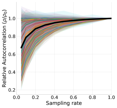
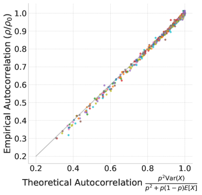
Figure 4: Empirical and theoretical effects of sampling on autocorrelation of hashtag popularity. (left) Median autocorrelation relative to the original time series for 100 most popular hashtags; shaded regions mark the inter-quartile ranges; the black line represents the average autocorrelation across all hashtags. (right) Accuracy of the theoretical prediction according to Equation 3.

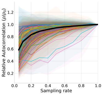
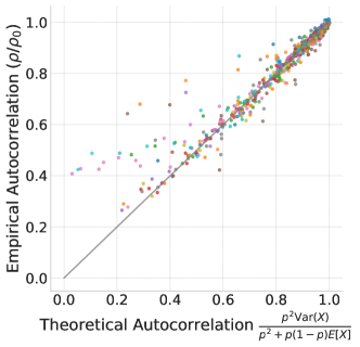
Figure 21: Empirical and theoretical effects of sampling on autocorrelation of user’s activity. The left plot shows the median autocorrelation relative to the original time series for each of the top 100 most active users; shaded region marks the interquartile ranges; the black line represents the average autocorrelation across all users. The right plot shows the accuracy of the theoretical prediction according to Equation 3. The line depicts the identity function to represent an accurate fit to the data.

Figure 4 (left) shows the effects of sampling at different rates on the autocorrelation of hashtags’ popularity. The plot shows the median autocorrelation loss relative to the original time series. For each ground truth signal, we found the most significant autocorrelation time lag, which is kept fixed during the down sampling process to calculate autocorrelation at different sampling rates; then, we plotted the median ratio between the original and sampled autocorrelation. Although the curvatures are different for each hashtag, all time series are accurately characterized by our theoretical results (Equation 3): Figure 4 (right) shows that the empirical loss of autocorrelation fits the theoretical predictions. Figure 21 (SI) reports the results for the sampled time series of Twitter user activity, measured by the daily number of user’s posts.

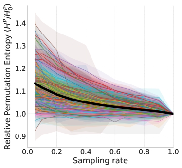
Figure 18: Loss of predictability in social media due to sampling on user’s activity (posts made by the user). The plot shows the median weighted permutation entropy relative to the original time series for each of the top 100 most popular hashtags.

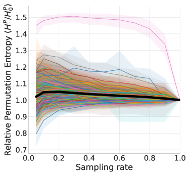
Figure 19: Loss of predictability in social media due to sampling on user’s activity (posts made by the user). The plot shows the median weighted permutation entropy relative to the original time series for each of the top 100 most active users.

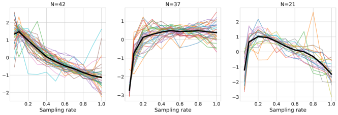
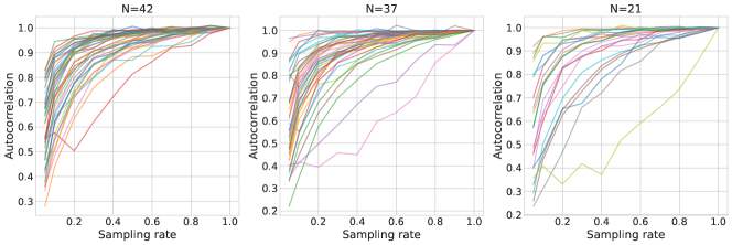
Figure 20: Clustering the permutation entropy behavior from Figure 19. We use, K-means clustering to depict the three most characteristics types of behaviors exhibited when computing predictability in social media as a function of sampling on user’s activity.

The loss of predictability is also seen when using permutation entropy with the same sampling strategy. Figures 18 and 19 (SI) show a clear trend in entropy increase (i.e., decrease of predictability) for both user activity and popularity of hashtags. The loss of predictability for user activity, for instance, happens in 63% of the users, while the rest of the cases comprise of time-series whose PE mostly do not change, except for low sampling rates (see Figure 20 (SI)).

Note that, in many applications, researchers use data from the Twitter Decahose or the streaming API, which capture approximately 10% and 1% sample of tweets, i.e., sampling rates of 0.1 and 0.01 respectively  (?). Considering that, at such low sampling rates, relative autocorrelation may be half of its value using the complete Twitter stream (Firehose), care should be taken when drawing conclusions from the partially observed system.

Cryptocurrency Popularity.

We present additional findings regarding loss of correlation between a sampled time series and an external signal. We study the effect of the price of cryptocurrencies on the adoption of said technology by software developers. To measure interest in the technology behind a cryptocurrency, we track the popularity of Github projects whose description is associated to that cryptocurrency. The four most popular cryptocurrencies during the collection period spanning January 2015 to March 2015 were Bitcoin (BTC), Litecoin (LTC), Monero (XMR) and Ripple (XRP). Some cryptocurencies, like Ethereum, were also popular, but since they were not yet publicly launched, we excluded them from the following analysis.

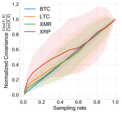
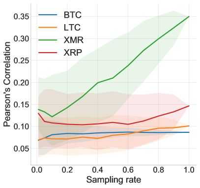
Figure 5: Loss of correlation between cryptocurrencies repository popularity and their prices for different sampling rates. Each point is the median Pearson’s correlation coefficient over $1000$ samples. Error bars show the standard deviation. For each cryptocurrency, we calculated over the $1000$ samples, (left) the median normalized covariance $\frac{\mathrm{Cov}(Y,S)}{\mathrm{Cov}(X,S)}$ and (right) the Pearson’s correlation coefficient between the price and the popularity of related Github repositories at different sampling rates. Shaded regions mark the inter-quartile ranges for each coin.

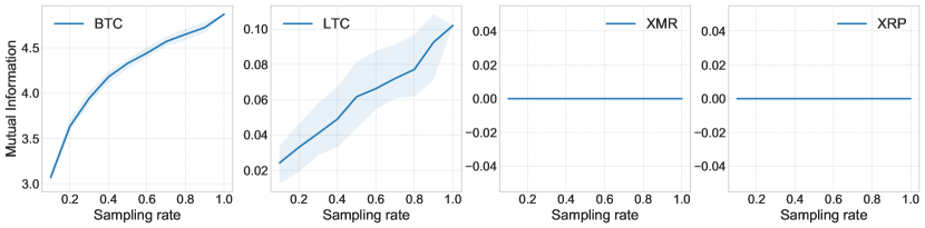
Figure 22: Decay of mutual information between the popularity of cryptocurrencies repositories and their prices for different sampling rates. For each cryptocurrency, and each sampling rate, we obtained $100$ samples, and calculated the median mutual information  (?) between the price and the popularity of related Github repositories. The solid line represents the median mutual information for each coin. Shaded region marks the interquartile ranges for each coin.

Figure 5 explores the effect that sampling has on the correlation. The left plot shows a clear decrease in the relative covariance for lower sampling rates, corroborating our theoretical results. As opposed to the behavior of influenza outbreaks (cf., Fig. 3), in Figure 5 (Right) we can see that a decay of covariance tends to induce a loss of correlation, especially for those coins with low variance relative to their mean. Supplementary Figure 22 depicts a decrease in mutual information for BTC and LTC, while the other two coins are independent of the external signal.

Synthetic Data.

Finally we investigate the impact of sampling on the predictability of synthetic data generated by an auto-regressive process (SI, Synthetic Data Experiments). In addition to autocorrelation and permutation entropy, we measure the error of forecasts made by an auto-regressive model trained on the sampled data. Similar to other metrics that demonstrate a loss of predictability, prediction error grows at lower sampling rates (SI, Figure 7). As a result, the forecasts made by auto-regressive models from data collected at low sampling rates are no more accurate than forecasts made by a Poisson model that assumes independent events. Sampling further distorts the observed dynamics of the auto-regressive process by introducing heteroskedasticity into the sampled time series. The time-varying variance causes predictions to deteriorate (SI, Synthetic Data Experiments, Proposition S2).

Materials and Methods

Permutation Entropy (PE).

We use permutation entropy as a model-free measure of predictability of a time series  (?, ?, ?). Permutation entropy captures the complexity of a time series via statistics of its ordered sub-sequences of the type $s=[x_{t},x_{t+\tau},\ldots,x_{t+(d-1)\tau}]$, given embedding dimension $d$ and a temporal delay $\tau$. Let $\mathcal{S}_{d,\tau}$ be the collection of all $d!$ permutations $\pi$ of size $d$ and temporal delay $\tau$. For each $\pi\in\mathcal{S}_{d,\tau}$, we determine the relative frequency $P(\pi)$ of that permutation occurring in the time series. The permutation entropy of order $d\geq 2$ and delay $\tau\geq 1$ is defined as

$$H^{\mathrm{P}}(d,{\tau})=-\sum_{\pi\in\mathcal{S}_{d,\tau}}P(\pi)\log_{2}P(\pi)$$ (1)

We use weighted permutation entropy  (?) to lessen the influence of observational noise on the ordinal pattern of the signal, in which weights with respect to a sub-sequence with a certain ordinal pattern are introduced to reflect the importance of ordinal changes in large amplitudes. Finally, we normalize weighted permutation entropy by dividing it by $\log_{2}(d!)$, log of the number of possible permutations. See SI, Permutation Entropy Criterion, for a formal definition. To estimate PE of a time series we need to specify the order $d$ and time delay $\tau$. The optimal parameters will depend on the specific properties of the time series, for example, the periodic behavior of the system relates to the delay parameter  (?). Here, we follow the approach described in  (?), which performs a grid search over the pairs $(d,\tau)$, $2\leq d\leq 5$ and $1\leq\tau\leq 7$ searching for the values that minimize $H^{\mathrm{P}}(d,\tau)$. However, for the parameter search, PE is normalized by the number of observed permutations instead of the possible permutations, given that otherwise, $H^{\mathrm{P}}(d,\tau)$ is decreasing as a function of $d$. Finally, the parameters found for each ground truth signal are used to compute the PE of the corresponding sampled time series.

Mutual Information

Mutual information characterizes the amount of information one random variable contains about another, specifically capturing the reduction in the uncertainty of one random variable due to the knowledge of the other. The mutual information between two random variables is defined as $\displaystyle I(X;Y)=\mathbb{E}_{p(x,y)}\ln\frac{p(X,Y)}{p(X)p(Y)}$.

Here we consider the mutual information between two time series. We calculate the mutual information between two time series with PyInform  (?).

Loss of autocorrelation of the Sampled Signal.

Our first theoretical result shows that sampling reduces the auto-covariance of the observed signal, i.e., the covariance of the time series $Y$ and its time-lagged version.

Theorem 1.

The time series $X$, $Y$ are related by $Y\sim B([X],p)$, where $B([X],p)$ is a Bernoulli random process with success rate $p$.

The covariance matrices $\boldsymbol{\Sigma}_{X}$ and $\boldsymbol{\Sigma}_{Y}$ are related as

$$\boldsymbol{\Sigma}_{Y}=p^{2}\boldsymbol{\Sigma}_{X}+p(1-p)\mathbb{E}[X]\boldsymbol{I}$$ (2)

where $\boldsymbol{I}$ is the identity matrix.

We can use the expression in Theorem 1 to approximate the autocorrelation of the sampled time series $Y$ as a function of the ground truth signal $X$. Autocorrelation is defined as Pearson correlation between values of the signal at different times, i.e., $\rho_{X_{i},X_{j}}=\frac{\mathrm{Cov}(X_{i},X_{j})}{\sigma_{X_{i}}\sigma_{X_{j}}}.$ For sake of simplicity, we assume that the ground truth process is stationary.

Corollary 1.

The autocorrelation of sampled time series $Y$ is

$$\rho_{Y_{i},Y_{j}}\approx\frac{p^{2}\mathrm{Cov}(X_{i},X_{j})}{p^{2}\mathrm{Var}(X)+p(1-p)\mathbb{E}[X]}.$$ (3)

Corollary 2.

The magnitude of autocorrelation $|\rho_{Y_{i},Y_{j}}|$ of the observed signal $Y$, increases monotonically as a function of the sampling rate $p$.

Corollary 3.

The covariance between the observed signal $Y$ and an arbitrary external signal $S$ is related to the covariance between the ground truth signal $X$ and the same external signal $S$ by,

$$\mathrm{Cov}(Y,S)=p\,\mathrm{Cov}(X,S).$$ (4)

Epidemics Data.

Weekly state-level data for all diseases was obtained from Scarpino & Petri  (?) and originally compiled by the USA National Notifiable Diseases Surveillance System (see SM, Table 1 for statistics of the data). For the covariance experiment, we used influenza data from 2010-2015 obtained for the US Outpatient Influenza-like Illness Surveillance Network (ILINet) that overlaps with Google Flu Trends Data.

Twitter Data.

The social media data used in this study was collected from Twitter in 2014. Starting with a set of 100 users who were active discussing ballot initiatives during the 2012 California election, we expanded this set by retrieving the accounts of the users they followed, for a total of 5,599 seed users. We collected all posts made by the seed users and their friends (i.e., users they followed on Twitter) over the period of June–November 2014, a total of over 600 thousand users. We extracted time series of the activity for 100 most popular hashtags and 150 most active users in this data (see SM, Tables 2 and 3 for statistics of the data).

GitHub Data.

The GitHub data we analyzed contains anonymized records of user activities over a time period spanning from January 1st, 2015 to March 31st, 2015. The activities represent the actions users performed on the repositories, including watching the repositories to receive notifications about project activity. We used watches, forks, and create event activity as a measure of popularity of a repository in Github. Overall, our dataset captures $43,962$ Github activity events by $5,509$ users on $2,036$ repositories (see Supplementary Information (SI), Table 4 for additional statistics). Cryptocurrencies’ historical prices were obtained from publicly available Kaggle datasets.

Discussion

We presented a framework to analyze the effects of partial observation of a dynamic process, showing that sampling degrades the predictability of the process. Using empirical data from three domains, namely epidemics, social systems, and software collaborations, we highlighted how this fundamental predictability limit affects the forecasting of disease outbreaks, social media content popularity, and emergence of cryptocurrency technologies. We showed that even when events making up the temporal signal are sampled at random, sampling qualitatively changes the observed dynamics of the process, decreasing the autocorrelation and increasing permutation entropy. Moreover, the predictability loss is irreversible: even a highly informative external signal does not help to fully recover predictability lost to sampling. These findings were corroborated by experiments on synthetic data.

Our work is motivated by applications requiring the forecasting of partially observed, or sampled, complex systems. Such situations may occur, for example, when country-wide forecasts of influenza have to be made based on reports by a few hospitals; when longitudinal opinion polls of a population are used to predict an election; or when researchers avail of random samples of social media activity to characterize complex social dynamics. Beyond prediction, models learned from data can also elucidate social behaviors  (?). Scientists developed techniques for temporal data analysis, based on anomaly detection  (?) and regression discontinuity design  (?), to uncover natural experiments that yield insights into the mechanisms of human decision making. As we showed in this paper, however, these techniques may be systematically biased by temporal sampling. It is, therefore, imperative to account for potential sampling biases in the study of social dynamics, so that no results are erroneously attributed to the phenomena under study. Thus, it is important for future research to focus on statistical tools and sampling methods that can correct for these possible biases.

Our work suggests that partial observability not only diminishes the predictability of a dynamic process, but also introduces a source of heterogeneous random noise that can potentially mislead causal inference methods and threaten their validity. For example, interrupted time series (ITS) analyses is one of the most widely applied approaches to evaluate natural experiments in health interventions  (?). ITS consists of a sequence of counts over time, with one or more well-defined change points that correspond to the introduction of an intervention. The effect of the intervention can be estimated by fitting a linear regression model with a dummy variable for the before/after intervention, and additional variables to control for time-varying confounders. Only recently, researches have addressed methodological issues associated with ITS analysis caused by over-dispersion of time series data and autocorrelation  (?). For instance, a study estimating the impact of a ban on the offer of multipurchase discounts by retailers in Scotland, found a 2% decrease in alcohol sales after controlling for seasonal autocorrelation, compared with a previous study’s finding no impact  (?). Our work provides a theoretical framework to understand and quantify new sources of biases that sampling creates that can affect intervention studies.

Code Availability

Codes to generate the results of the paper are available on https://github.com/aabeliuk/Predictability-partially-observed.

Data Availability

This work uses publicly available data. Links to data repositories can be found in the Methods section.

Acknowledgments

The authors thank Linhong Zhu for collecting the Twitter data and America Mazuela for the illustration. Funding: This work was supported by the Office of the Director of National Intelligence (ODNI) and the Intelligence Advanced Research Projects Activity (IARPA) via the Air Force Research Laboratory (AFRL) contract number FA8750-16-C- 0112, and by the Defense Advanced Research Projects Agency (DARPA), contract number W911NF-17-C-0094. The U.S. Government is authorized to reproduce and distribute reprints for Governmental purposes notwithstanding any copyright annotation thereon. Disclaimer: The views and conclusions contained herein are those of the authors and should not be interpreted as necessarily representing the official policies or endorsements, either expressed or implied, of ODNI, IARPA, AFRL, DARPA, or the U.S. Government. Authors contributions: All authors conceptualized the study; ZH carried out formal analysis; AA carried out validations with empirical data; ZH and AA carried out validations with synthetic data; all authors contributed to writing and reviewing the manuscript. Competing interests: Authors declare no competing interests.

Supplementary Information (SI)

Proofs to Propositions and Corollaries

Proof of Theorem 1

Theorem 2 (Restatement of Theorem 1).

The time series $X$, $Y$ are related by $Y\sim B([X],p)$, where $B([X],p)$ is a Bernoulli random process with success rate $p$. The covariance matrices $\boldsymbol{\Sigma}_{X}$ and $\boldsymbol{\Sigma}_{Y}$ are related as

$$\boldsymbol{\Sigma}_{Y}=p^{2}\boldsymbol{\Sigma}_{X}+p(1-p)\mathbb{E}[X]\boldsymbol{I}$$

where $\boldsymbol{I}$ is the identity matrix.

Proof.

First, we compute the off-diagonal elements of covariance matrices $\boldsymbol{\Sigma}_{Y}$ and $\boldsymbol{\Sigma}_{X}$, i.e., the relation between $\mathrm{Cov}(X_{i},X_{j})$ and $\mathrm{Cov}(Y_{i},Y_{j})$.

$$\mathrm{Cov}(Y_{i},Y_{j}) =\mathbb{E}[Y_{i}Y_{j}]-\mathbb{E}[Y_{i}]\mathbb{E}[Y_{j}]$$

$$=\mathbb{E}_{X}\big{[}\mathbb{E}_{Y}[Y_{i}Y_{j}|X_{i},X_{j}]\big{]}-\mathbb{E}_{X}\big{[}\mathbb{E}_{Y}[Y_{i}|X_{i}]\big{]}\mathbb{E}_{X}\big{[}\mathbb{E}_{Y}[Y_{j}|X_{j}]\big{]}$$

$$=\mathbb{E}_{X}\big{[}\mathbb{E}_{Y}[Y_{i}|X_{i}]\mathbb{E}_{Y}[Y_{j}|X_{j}]\big{]}-$$

$$\phantom{{}=1}\mathbb{E}_{X}\big{[}\mathbb{E}_{Y}[Y_{i}|X_{i}]\big{]}\mathbb{E}_{X}\big{[}\mathbb{E}_{Y}[Y_{j}|X_{j}]\big{]}$$

$$=\mathbb{E}_{X}\big{[}p^{2}[X_{i}][X_{j}]\big{]}-\mathbb{E}_{X}\big{[}p[X_{i}]\big{]}\mathbb{E}_{X}\big{[}p[X_{j}]\big{]}$$

$$=p^{2}\big{(}\mathbb{E}\big{[}[X_{i}][X_{j}]\big{]}-\mathbb{E}\big{[}[X_{i}]\big{]}\mathbb{E}\big{[}[X_{j}]\big{]}\big{)}$$

$$\approx p^{2}\mathrm{Cov}(X_{i},X_{j})$$ (5)

Next, we discuss diagonal elements, i.e., the relation between $\mathrm{Var}[Y]$ and $\mathrm{Var}[X]$. Without loss of generality, normal approximation will be used: $Y\sim B([X],p)$ is approximated by $Y\sim\mathcal{N}([X]p,[X]p(1-p))$. Thus, for fixed $X$, $\displaystyle Z\equiv\frac{Y-pX}{\sqrt{p(1-p)X}}\sim\mathcal{N}(0,1)$, then $\displaystyle Z^{2}=\frac{Y^{2}-2pYX+p^{2}X^{2}}{p(1-p)X}\sim\chi^{2}(1)$, i.e.,

$$\mathbb{E}[Z^{2}]=\mathbb{E}\bigg{[}\frac{Y^{2}-2pYX+p^{2}X^{2}}{p(1-p)X}\bigg{]}=1$$

This gives $\mathbb{E}[Y^{2}|X]=p(1-p)X+2p\mathbb{E}[Y|X]X-p^{2}X^{2}=p(1-p)X+p^{2}X^{2}$

$$\mathrm{Var}[Y] =\mathrm{Cov}(Y,Y)=\mathbb{E}[Y^{2}]-\mathbb{E}[Y]^{2}$$

$$=\mathbb{E}_{X}\big{[}\mathbb{E}_{Y}[Y^{2}|X]\big{]}-\mathbb{E}_{X}\big{[}\mathbb{E}_{Y}[Y|X]\big{]}^{2}$$

$$=\mathbb{E}_{X}[p(1-p)X+p^{2}X^{2}]-\mathbb{E}_{X}[pX]^{2}$$

$$=\mathbb{E}_{X}[p(1-p)X+p^{2}X^{2}]-p^{2}\mathbb{E}_{X}[X]^{2}$$

$$=p(1-p)\mathbb{E}[X]+p^{2}\mathrm{Var}[X]$$ (6)

Equations (5) and (6) give the desired result. ∎

Proof of Corollary 1

Proof.

Autocorrelation is defined as Pearson correlation between values of the signal at different times, i.e.,

$$\rho_{X_{i},X_{j}}=\frac{\mathrm{Cov}(X_{i},X_{j})}{\sigma_{X_{i}}\sigma_{X_{j}}}.$$

This yields the following expression for autocorrelation of the time series $Y$:

$$\rho_{Y_{i},Y_{j}}=\frac{\mathrm{Cov}(Y_{i},Y_{j})}{\sigma_{Y_{i}}\sigma_{Y_{j}}}=\frac{p^{2}\mathrm{Cov}(X_{i},X_{j})}{\sqrt{p^{2}\mathrm{Var}(X_{i})+p(1-p)\mathbb{E}[X_{i}]}\sqrt{p^{2}\mathrm{Var}(X_{j})+p(1-p)\mathbb{E}[X_{j}]}}.$$ (7)

The last equality comes from replacing Equation 5 in the numerator and Equation 6 in the denominator. Finally, we assume the ground truth process is stationary, i.e., the process has a time-independent variance ($\mathrm{Var}(X_{j})\approx\mathrm{Var}(X_{j})\;\forall i,j$) and mean ($\mathbb{E}(X_{j})\approx\mathbb{E}(X_{j})\;\forall i,j$), yielding the desired result:

$$\rho_{Y_{i},Y_{j}}\approx\frac{p^{2}\mathrm{Cov}(X_{i},X_{j})}{p^{2}\mathrm{Var}(X)+p(1-p)\mathbb{E}[X]}.$$ (8)

∎

Proof of Corollary 2

Proof.

Based on Corollary 1, the autocorrelation of the sampled signal $Y$ between times $i$ and $j$, which is a function of sampling rate $p$, is defined as

$$R(p)=\rho_{Y_{i},Y_{j}}=\frac{p^{2}\mathrm{Cov}(X_{i},X_{j})}{\sqrt{p^{2}\mathrm{Var}(X_{i})+p(1-p)\mathbb{E}[X_{i}]}\sqrt{p^{2}\mathrm{Var}(X_{j})+p(1-p)\mathbb{E}[X_{j}]}}.$$ (9)

The autocorrelation lies in the range $[-1,1]$, and we want to prove that its magnitude increases as a function of $p$. Hence, next we show that $\frac{\mathrm{d}}{\mathrm{d}p}R^{2}(p)\geq 0,\forall 0\leq p\leq 1$.

$$\frac{\mathrm{d}}{\mathrm{d}p}R^{2}(p)=p\;\mathrm{Cov}(X_{i},X_{j})^{2}\frac{\mathrm{Var}(X_{i})\mathbb{E}[X_{j}]p+\mathbb{E}[X_{i}]\mathrm{Var}(X_{j})p+2\mathbb{E}[X_{i}]\mathbb{E}[X_{j}](1-p)}{\left(\mathrm{Var}(X_{i})p-\mathbb{E}[X_{i}]p+\mathbb{E}[X_{i}]\right)^{2}\left(\mathrm{Var}(X_{j})p-\mathbb{E}[X_{j}]p+\mathbb{E}[X_{j}]\right)^{2}},$$ (10)

where both the numerator and denominator are trivially positive for all values in $0\leq p\leq 1$ given that $\mathbb{E}[X]\geq 0$, and the result follows. ∎

Proof of Corollary 3

Proof.

We compute the covariance between sampled signal $Y$ and external signal $S$ as

$$\mathrm{Cov}(Y,S) =\mathbb{E}(Y-\mathbb{E}Y)(S-\mathbb{E}S)$$

$$=\mathbb{E}[YS]-\mathbb{E}[Y]\mathbb{E}[S]$$

$$=\mathbb{E}_{X,S}\big{[}S\mathbb{E}_{Y}[Y|S,X]\big{]}-\mathbb{E}_{X}\big{[}\mathbb{E}_{Y}[Y|X]\big{]}\mathbb{E}[S]$$

$$=\mathbb{E}_{X,S}[SXp]-\mathbb{E}_{X}[Xp]\mathbb{E}[S]$$

$$=p\big{(}\mathbb{E}[SX]-\mathbb{E}[X]\mathbb{E}[S]\big{)}$$

$$=p\,\mathrm{Cov}(X,S)$$ (11)

∎

Permutation Entropy Criterion

Entropy measures the uncertainty of a random variable, which intuitively serves as an indicator of predictability of a stochastic event. In statistical physics, entropy characterizes the amount of possible microscopic state in a system, thus the more microscopic states exist in a system, the more chaotic a system is, and the harder it becomes to predict its behavior.

Definition 3 (Shannon entropy).

For a random variable, the (Shannon) entropy is defined as

$$\textrm{discrete case: }H(p) =-\sum_{x\in\mathcal{X}}p(x)\ln p(x)$$ (12)

$$\textrm{continuous case: }H(p) =-\int_{S}p(x)\ln p(x)\,\mathrm{d}x$$ (13)

$p(x)$ is the probability distribution of the random variable. In the discrete case, $\mathcal{X}$ is the collection of all possible values of the random variable. In the continuous case, $S$ is the support set of the random variable.

In both discrete and continuous case, the larger the entropy value is, the more uncertain a random variable is, thus rendering the stochastic event a random variable represents harder to predict. A variant form of entropy is the permutation entropy, which depicts the complexity of a time series through the statistics of of the values of its subsequences using ordinal analysis. The complexity can be interpreted as the diversity of the trends among the subsequences of certain length. Therefore, the higher the entropy, the more different trends exist in the time series, which renders its prediction more difficult.

Permutation entropy has been used in various fields to characterize the predictability of time series under interest  (?, ?). Interestingly, this quantity has also been used as a forensic tool to inspect and identify potential corruption in the source data  (?).

Definition 4 (Permutation Entropy).

Given a time series $\{x_{t}\}_{t=1}^{N}$. Let $\mathcal{S}_{d}$ be the collection of all $d!$ permutations $\pi$ of order $d$. For each $\pi\in\mathcal{S}_{d}$, determine the relative frequency of that permutation occurring in $\{x_{t}\}_{t=1}^{N}$:

$$P(\pi)=\frac{\mathrm{Card}[\{t\,|\,t\leq N-d,\phi(x_{t+1},\cdots,x_{t+d})=\pi\}]}{N-d+1}=\sum_{t\leq N-d}\frac{1}{N-d+1}\delta\big{(}\phi(x_{t+1}^{(d)}),\pi\big{)}$$

where $P(\pi)$ quantifies the frequency of an ordinal pattern $\pi$, and $\delta(a,b)=\begin{cases}1,\,&\textrm{if }a=b\\ 0,\,&\textrm{if }a\neq b\end{cases}$.

The permutation entropy of order $d\geq 2$ is defined as

$$H^{\mathrm{P}}(d)=-\sum_{\pi\in\mathcal{S}_{d}}P(\pi)\log_{2}P(\pi)$$ (14)

The ordinal pattern means the relative magnitude relation among successive time series values. As an example, if $x_{1}=3,x_{2}=6,x_{3}=1$, then the ordinal pattern of this subsequence $\{x_{1},x_{2},x_{3}\}$ is $\phi(x_{1},x_{2},x_{3})=(312)$ because $x_{3}\leq x_{1}\leq x_{2}$.

Besides the order $d$, the more general definition of permutation entropy (1) has one more parameter: temporal delay $\tau$. The ordinal pattern can be defined in the same way with respect to the subsequence $x_{t},x_{t+1\tau},x_{t+2\tau},\cdots,x_{t+(d-1)\tau}$, which gives permutation entropy $H^{\mathrm{P}}(d,\tau)$. To facilitate interpretation, we present results from continuous intervals by fixing $\tau=1$.

To lessen the influence of observational noise on the ordinal pattern of the signal, the weight w.r.t. a subsequence with certain ordinal pattern is introduced to reflect the importance of ordinal changes in large amplitude. For a subsequence of length/order $d$ consisting times series values from $x_{t+1}$ to $x_{t+d}$, which is denoted as $x_{t+1}^{(d)}$ with arithmetic mean value $\bar{x}_{t+1}^{(d)}$, its weight is defined  (?) as

$$w(x_{t+1}^{(d)})=\frac{1}{d}\sum_{j=t+1}^{t+d}(x_{j}-\bar{x}_{t+1}^{(d)})^{2}$$

As a result, the weighted frequency of a permutation is defined as

$$P_{w}(\pi)=\sum_{t\leq N-d}\bigg{(}\frac{w(x_{t+1}^{(d)})}{\sum_{t^{\prime}\leq N-d}w(x_{t^{\prime}+1}^{(d)})}\bigg{)}\delta\big{(}\phi(x_{t+1}^{(d)}),\pi\big{)}$$

The weighted permutation entropy is defined as

$$H^{\mathrm{P}}_{(w)}(d)=-\sum_{\pi\in\mathcal{S}_{d}}P_{w}(\pi)\log_{2}P_{w}(\pi)$$ (15)

Here we normalize the weighted permutation entropy by the log-number of the factorial of the observed permutations. Thus, the weighted permutation entropy takes value between 0 and 1.

Synthetic Data Experiments

Here, we validate our findings on synthetically generated time series data. We show that predictability diminishes as data is lost to sampling. We first consider an idealized scenario, where $X$ represents an autoregressive process, from which events are sampled at random to create the observed sampled signal $Y$.

Synthetic Time Series Generation

External Signal

First, we generate an external signal $S$. To assure autocorrelation, we generate it using the autoregressive integrated moving average (ARIMA) model:

$$S+\sum_{i=1}^{k}\alpha_{i}^{\textrm{ES}}S_{t-i}=\varepsilon_{t}+\sum_{j=1}^{l}\beta_{j}^{\textrm{ES}}\varepsilon_{t-j}.$$ (16)

ARIMA coefficients satisfy the stationarity conditions, so that the external signal $S$ is second-order stationary. The stationarity conditions require that all roots of the polynomials $\alpha(x)=1+\alpha_{1}x+\cdots+\alpha_{k}x^{k}$ and $\beta(x)=1+\beta_{1}x+\cdots+b_{l}x^{l}$ satisfy $|z|>1$; i.e., all roots of these two polynomials are located outside the unit disk. We enforce the second order stationarity by determining roots of $\alpha(x)$ and $\beta(x)$ first and then solving for the corresponding regression coefficients $\{\alpha_{i}\}$ and $\{\beta_{j}\}$, which specify the model.

Ground Truth Signal

We generate the ground truth signal $X$ in a similar manner, except that the generation model entails a term for the external signal $S$. This ensures that the ground truth and the external signals are correlated. Specifically, we assume the ground truth signal is defined as:

$$X+\sum_{i=1}^{K}\alpha_{i}^{\textrm{GT}}X_{t_{i}}=\varepsilon_{t}+\sum_{j=1}^{L}\beta_{j}^{\textrm{GT}}\varepsilon_{t-j}+S.$$ (17)

When generating the ground truth signal time series, we require that the autocorrelation of the ground truth signal is strong enough so that it can be distinguished from the random white noise.

Observed signal

We sample the ground truth data $X$ to obtain the time series of observed events, $Y$. The sampling rate $p$ characterizes the probability of sampling an event. Because the count process is described by the ARIMA model, which inevitably gives real-number-valued count instead of integer-valued count, the decimal part of the count $X$ is treated as a separate instance, and if the decision is made to keep it, its original value will be added to the posterior data. In other words, each instance of $Y$ obeys the Binomial distribution $B(X,p)$.

Due to the stochastic nature of sampling, we generate ten different samples $Y$ based on the ground truth signal with the same sampling rate $p$. In each experiment, the sampled signal $Y$ is split into a training and testing data set, with training data used to train a predictor $\hat{Y}$ to predict the test data. The accuracy of the predictor for a given sampling rate is then averaged over the ten experiments.

Model Training

Training an ARIMA model consists of two steps: First, a grid search is performed to find the best hyper-parameters $(k,l)$, where $k$ is the order of the autoregressive model, and $l$ is the order of the moving-average model. For each input signal, we search over the grid for the set of parameters resulting in the lowest AIC score. Next, the corresponding coefficients of the fixed-order ARIMA model are fitted to the data.

After the best ARIMA order parameters are determined, we do step by step prediction over a specified time range. At each prediction step, the data from the previous step is incorporated into the known data as new input signal, and consequently, the model is retrained to find the updated parameters.

Prediction

In order to compare predictions at different sampling rates, we use normalized rooted-mean-square error (NRMSE) to measure how accurately we predict the observable $Y$. Given the predicted values $\hat{y}_{t}$ with respect to time series $Y$, NRMSE is defined as

$$\mathrm{NRMSE}(y_{t},\hat{y}_{t}) =\frac{1}{\bar{y}}\sqrt{\frac{\sum_{i=1}^{T}(y_{i}-\hat{y}_{i})^{2}}{T}}$$

$$=\frac{1}{\frac{1}{T}\sum_{i=1}^{T}y_{i}}\sqrt{\frac{\sum_{i=1}^{T}(y_{i}-\hat{y}_{i})^{2}}{T}}$$ (18)

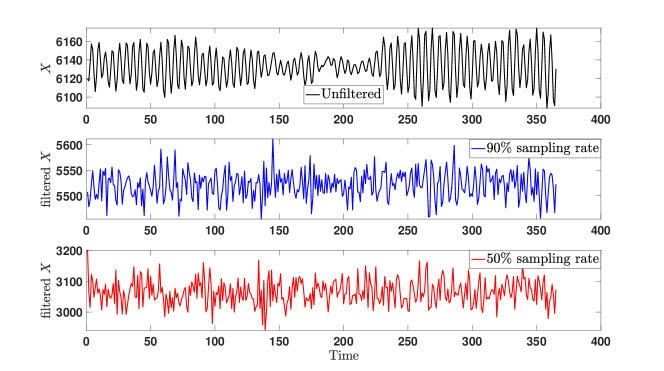
Figure 6: Synthetic time series showing ground truth signal (top) and the observed signal sampled at sampling rates $90\%$ (middle) and $50\%$ (bottom).

Numeric Experiments

First, we illustrate all our theoretical claims using one instance of an ARIMA process generated with an external signal. Second, we present aggregated results of the prediction task, using multiple randomly generated ARIMA time series.

For the first set of results on the synthetic data, we generated an external signal $S$ with the ARIMA of order (3,0,2) and length 365, representing a full year of event counts.

Meanwhile, the ground truth signal $X$ assumes the ARIMA order(5,0,1).

Figure 6 shows the ground truth and the sampled signals. Notice that with a simple visual inspection of the plot, one can observe that many of the temporal patterns present in the unsampled data seem to have disappeared in the sampled signal.

Predictors

We train three predictors for $Y$, each of which can be used with or without an external signal. The predictors are:

Poisson predictor

assumes that events in $Y$ are generated independently of each other at some rate. This predictor estimates the Poisson intensity as the average of counts of all available past data.

$\boldsymbol{\hat{Y}_{t}}$

uses the sampled signal to predict the observable $Y$.

$\boldsymbol{\hat{X}_{t}}$

uses the unsampled signal to predict the observable $Y$. i.e., the ARIMA parameters are fitted to $X$, and then used to predict the future values of $Y$ given its past values.

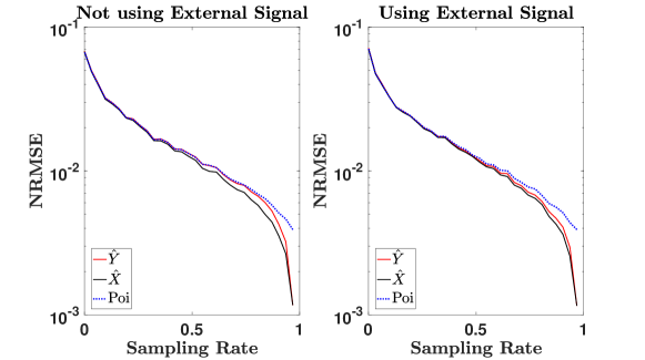
Figure 7: Prediction accuracy in terms of NRMSE, and the difference in prediction performance among different predictors versus Sampling Rate Plot. Here we use three predictors to estimate sampled counting process $Y$.

Prediction Accuracy

Figure 7 shows normalized prediction errors (normalized RMSE) as a function of sampling rate to demonstrate the nonlinear decrease of the prediction error. As sampling rate decreases, prediction error grows. We study the performance of the predictor $\hat{Y}$, which is trained on the history of the observed signal $Y$, as it is often employed in practice.

Performance of the predictor $\hat{X}$, trained on the full signal $X$, is almost always better (lower NRMSE) than performance of predictor $\hat{Y}$ (the plot show difference between predictors on the log scale). This phenomenon reveals that sampling weakens prediction accuracy. Moreover, our results suggest that the sampled process’ increased noise and low autocorrelation obfuscates the underlying dynamic, making it harder to be described by an ARIMA model. Using an informative external signal $S$ in prediction helps recover some of the lost information, shrinking the gap between $\hat{X}$ and $\hat{Y}$ predictors, as well as the overall prediction error.

When little information is lost (i.e., at high sampling rate), predictors $\hat{X}$ and $\hat{Y}$ outperform the Poisson predictor, since they are able to leverage the autocorrelation of the signal with the ARIMA model. In addition, by comparing the gaps between predictors at high sampling rates (note the log scale), we see that adding external signal makes the Poisson predictor less competitive than the other predictors. On the other hand, Poisson predictor performs almost as well as $\hat{Y}$ and $\hat{X}$ when much of the information is lost (i.e., at low sampling rate). This indicates that Poisson predictors are strong baselines for the observable $Y$ at low sampling rates.

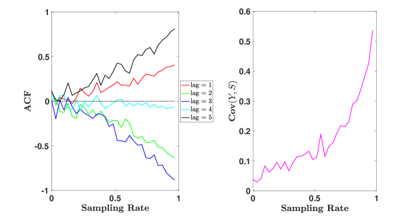
Figure 8: Loss of predictability due to sampling. (left) autocorrelation of sampled time series decreases at low sampling rates. (right) Covariance of the external signal and observed signal decreases at low sampling rates.

Loss of autocorrelation

Figure 8 shows that the autocorrelation of the sampled signal increases with sampling rate, consistent with Corollary 2. This figure shows that sampling at low rate quickly destroys the innate autocorrelation of the signal, fundamentally altering the properties of the signal and rendering the prediction task harder. We also see that the correlation between sampled ground truth signal $Y$ and the external signal gradually increases in agreement with Corollary 3. As a consequence of the loss of autocorrelation and correlation with the external signal, we can observe in Figure 7, that at low sampling rates, the accuracy of the Poisson predictor is competitive to the ARIMA predictors.

Increase in Permutation Entropy

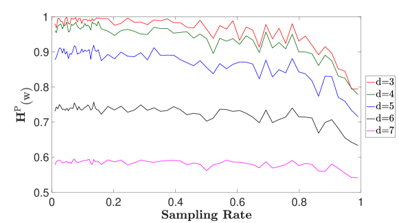
Figure 9: Loss of predictability due to sampling for the synthetic data shown in Figure 6. Normalized weighted permutation entropy with respect to sampling rate increases at low sampling rates, showing the system becomes less predictable. Parameter $d$ is the embedded time dimension used to compute corresponding weighted permutation entropy $H^{\mathrm{P}}_{(\textrm{w})}$. The delay dimension is set to $\tau=1$.

Figure 9 shows that the weighted permutation entropy decreases at high sampling rates, when more of the signal is retained. This shows the loss of predictability of the process at low sampling rates. The trends in the figure imply that even when little of the signal is filtered out, its predictability significantly degrades.

Decrease in Mutual Information

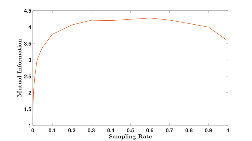
Figure 10: Decay of mutual information between the external signal and the sampled signal. Although the external signal in this illustration is highly correlated with the original (unfiltered) ground truth signal, sampling leads to a sharp loss of information about the original signal.

The loss of predictability cannot be offset using an informative external signal. This is because even if the external signal is highly correlated with the ground truth signal, sampling reduces its utility in predictive tasks. Figure 10 shows this decay in mutual information between the external and observed signals at low sampling rates. The informative external signal does not reduce the uncertainty of the observed signal.

Nonstationarity of Prediction Errors

Another quantity that characterizes the impact of sampling on the predictability of a time series is the covariance of the prediction error at different times, as the prediction error can intuitively reflect how well one can predict the event count. We show that sampling the time-series will introduce an autocorrelation into the prediction error and render it dependent on the evolution of the counting process, with errors growing larger or smaller depending on the type of process. Next, we provide an example to motivate how sampling can induce a correlation between variances of predictions at different times.

Proposition S2.

Consider an auto-regressive (AR) process: $X_{t}=\alpha X_{t-1}+\varepsilon_{t},$ with $\varepsilon_{t}$ white noise. The variance at the next step is given by,

$$\mathrm{Var}(Y_{t}|X_{t})=\alpha\mathrm{Var}(Y_{t-1}|X_{t-1})+\varepsilon^{\prime}_{t}.$$

Proof.

The information filter can be described as a Binomial distribution, $Y\sim B(X,p)$. Hence, $\mathrm{Var}(Y_{t-1}|X_{t-1})=X_{t-1}p(1-p)$ using the fact that $Y_{t-1}|X_{t-1}$ is a Bernoulli random variable. Then, the variance at the next step is given by,

$$\mathrm{Var}(Y_{t}|X_{t})= X_{t}p(1-p)$$

$$= \left(\alpha X_{t-1}+\varepsilon_{t}\right)p(1-p)$$

$$= \alpha X_{t-1}p(1-p)+\varepsilon^{\prime}_{t}$$

$$= \alpha\mathrm{Var}(Y_{t-1}|X_{t-1})+\varepsilon^{\prime}_{t}.$$

∎

Proposition S2 shows that the variances of the sampled process, $Y$, are related by the exact same AR model that generated the process $X$. In other words, the conditional variance of the sampled process is autocorrelated. Notice, that this is not true for the unsampled data, given that $\mathrm{Var}(X_{t}|X_{t-1})=\mathrm{Var}(\varepsilon_{t})=\sigma^{2}$.

Proposition S2 shows that sampling a time series may introduce autoregressive conditional heteroskedasticity (ARCH) of the variance into the time series. This is usually tested by analyzing the residuals of the model. We use Engle’s Langrage Multiplier test to demonstrate the appearance of ARCH effects in the residual signal. Figure 11 shows that sampling does result in the introduction of ARCH effects to the residuals of predictions.

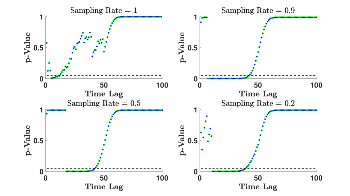
Figure 11: $p$-Value versus time lag

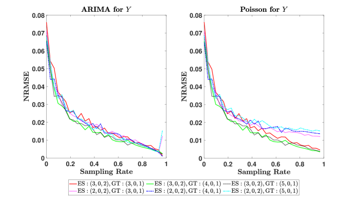
Figure 12: Change of prediction accuracy (RMSE) with respect to sampling rate for various ground truth signals, when the sampled GTs are predicted without knowing external signal $S$.

We have applied Engle’s Lagrange Multiplier (ELM) test  (?) on the residual $\hat{Y}-Y$, which is evaluated at time $t,t-1,\cdots,t-L$ where $L=100$ is the maximum time lag we consider, to examine the existence of ARCH behavior. Under the null hypothesis that there is no ARCH effect, the test statistic used in ELM test has the asymptotic distribution $\chi^{2}(L)$. When $p$-value is less than the significance level $\tilde{\alpha}=0.05$, the ELM test says that we can reject the null hypothesis with 95% confidence.

From Figure 11, we see that for the original time-series (top-left plot) there is no heteroskedasticity, $p$-values are largely over the significant level threshold $0.05$ for most of time lags under consideration. In the case of $q=0$, ELM test does not provide us enough evidence to reject the hypothesis that ARCH effect does not exist. However, when we filter the original signal, as we see in the case $q=0.1,0.5,0.8$ respectively, the $p$-value for time lags from 6 to 40 are mostly below the significance level bar, which, by ELM test, strongly suggests that the null hypothesis be rejected. In other words, ELM test suggests with 95% confidence that ARCH effect exists in the residual of prediction records on the filtered time-series.

Generalizability

So far, we have explored methodically one example where we have validated our theoretical results as well as provided new insights about the unpredictability of sampled time series. Here we show the average loss of predictability across many randomly generated ground truth time series.

We generate multiple external signal–ground truth signal pairs, and apply ARIMA and Poisson models on these data sets to test if the tendencies we have observed previously (i.e. nonlinear decrease of NRMSE with respect to sampling rate) will also appear in signals of different ARIMA orders. We observe in Figure 12 similar behavior across multiple data sets:

1. Increasing prediction error (NMRSE) despite small discrepancy at high sampling rates. This general behavior is partially due to the normalization by sample mean when we evaluate the NRMSE;

2. The autoregressive model outperforms the non-autoregressive Poisson model for higher sampling rates, but, this difference fades out for lower sampling rates as a consequence of sampling.

We further postulate that this decreasing tendency between increasing sampling rate and NRMSE bears generality with respect to any combination of ARIMA orders of external signal–ground truth data pair. When predicting $Y$ with the external signal $S$, we observe a very similar tendency of NRMSE—sampling rate relationship as in Figure 12. Albeit noticeable difference in the high end of sampling rate spectrum, the decreasing tendency, decreasing speed and the amplitude of NRMSE are by large the same as in the not-using-$S$ case.

In the general setting of ARIMA model, we show a decreasing prediction error w.r.t. the sampling rate, and the shrinking of the advantage of autoregressive model in prediction accuracy over Poisson model as sampling rate becomes smaller.

We demonstrated the decoupling of the external signal and the filtered signal as a prevalent phenomenon in the generic ARIMA setting. We observe in Figure 13 that for all ground truth-external signal pairs, the lower the sampling rate is, the smaller mutual information becomes. Therefore, we postulate that the positive correlation between sampling rate and mutual information can always be observed, thus implying that the knowledge of external signal cannot help recover the predictability of the ground truth signal.

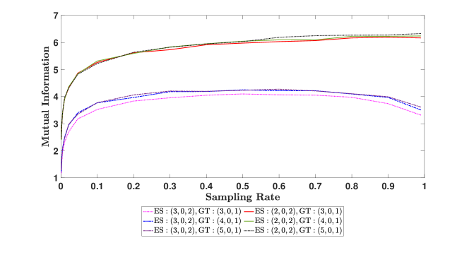
Figure 13: Change of mutual information (MI) with respect to sampling rate for various (ground truth, external signal) pairs.

Supplementary Figures

Epidemics.

Social Media.

Cryptocurrencies.

Supplementary Tables

Disease	Years	Total Infections	Infections/Year (SD)	Infections/week (SD)
Hepatitis	1966-2014	$742,554$	$15,154$ ($18,905$)	$14,011$ ($2,643$)
Influenza	1919-1951	$6,498,817$	$196,934$ ($198,551$)	$122,619$ ($163,348$)
Measles	1909-2001	$18,430,036$	$198,172$ ($247,833$)	$347,737$ ($310,744$)
Chlamydia	2006-2014	$4,882,110$	$542,456$ ($80,216$)	$92,115$ ($18,487$)
Polio	1921-1971	$505,246$	$9,907$ ($13,134$)	$9,532$ ($10,676$)
Gonorrhea	1972-2014	$3,701,913$	$86,091$ ($210,930$)	$69,847$ ($13,426$)
Mumps	1967-2014	$866,965$	$18,061$ ($35,054$)	$16,357$ ($9,180$)
Whooping cough	1909-2014	$2,220,008$	$20,943$ ($47,835$)	$41,887$ ($7,296$)

Table 1: Epidemics data: descriptive statistics.

Hashtags	Users	Tweets	Tweets/hashtag (SD)	Tweets/User (SD)	Tweets/Day (SD)
$100$	$233,108$	$1,269,348$	$12,693$ ($13,561$)	$5.4$ ($12$)	$11,135$ ($6,941$)

Table 2: Twitter hashtag activity descriptive statistics. Top 100 most popular hashtags.

Users	Tweets	Hashtags	Tweets/User (SD)	Tweets/hashtag (SD)	Tweets/Day (SD)
$150$	$167,654$	$20,990$	$1,118$ ($13,561$)	$8.0$ ($41.6$)	$1,552$ ($1,668$)

Table 3: Twitter user activity descriptive statistics. Top 150 most active users.

Cryptocurrency	Events	Repositories	Users	Events/Day (SD)	Events/Repo (SD)
Bitcoin (BTC)	$40,038$	$1,962$	$5,324$	$460$ ($116$)	$20.4$ ($138.4$)
Ripple (XRP)	$2,963$	$7$	$86$	$35.3$ ($27.7$)	$423.2$ ($1,115$)
Litecoin (LTC)	$1,222$	$137$	$302$	$14$ ($11$)	$8.9$ ($19.2$)
Monero (XMR)	$370$	$15$	$54$	$5.7$ ($6.3$)	$24.7$ ($55.8$)

Table 4: Github data: descriptive statistics.

References

- 1. A. Vespignani, Science 325, 425 (2009).
- 2. J. M. Hofman, A. Sharma, D. J. Watts, Science 355, 486 (2017).
- 3. C. Chatfield, Time-series forecasting (Chapman and Hall/CRC, 2000).
- 4. M. B. Short, et al., Mathematical Models and Methods in Applied Sciences 18, 1249 (2008).
- 5. G. O. Mohler, M. B. Short, P. J. Brantingham, F. P. Schoenberg, G. E. Tita, Journal of the American Statistical Association 106, 100 (2011).
- 6. N. Ramakrishnan, et al., Proceedings of the 20th ACM SIGKDD International Conference on Knowledge Discovery and Data Mining (2014), pp. 1799–1808.
- 7. V. Raghavan, A. Galstyan, A. G. Tartakovsky, The Annals of Applied Statistics pp. 2402–2430 (2013).
- 8. S. V. Scarpino, G. Petri, Nature communications 10, 898 (2019).
- 9. C. Song, Z. Qu, N. Blumm, A.-L. Barabási, Science 327, 1018 (2010).
- 10. R. D. Malmgren, D. B. Stouffer, A. S. Campanharo, L. A. N. Amaral, Science 325, 1696 (2009).
- 11. T. Hogg, K. Lerman, EPJ Data Science 1, 5 (2012).
- 12. G. Stoddard, Ninth International AAAI Conference on Web and Social Media (2015).
- 13. J. Garland, R. James, E. Bradley, Physical Review E 90, 052910 (2014).
- 14. J. Garland, et al., Entropy 20, 931 (2018).
- 15. N. I. Sapankevych, R. Sankar, IEEE Computational Intelligence Magazine 4, 24 (2009).
- 16. G. King, J. Pan, M. E. Roberts, Science 345, 1251722 (2014).
- 17. R. J. Little, D. B. Rubin, Statistical analysis with missing data, vol. 793 (Wiley, 2019).
- 18. F. Morstatter, J. Pfeffer, H. Liu, K. M. Carley, Seventh international AAAI conference on weblogs and social media (2013).
- 19. D. Ruths, J. Pfeffer, Science 346, 1063 (2014).
- 20. C. Bandt, G. Keller, B. Pompe, Nonlinearity 15, 1595 (2002).
- 21. B. Fadlallah, B. Chen, A. Keil, J. Príncipe, Physical Review E 87, 022911 (2013).
- 22. F. Pennekamp, et al., bioRxiv p. 350017 (2018).
- 23. D. G. Rand, S. Arbesman, N. A. Christakis, Proceedings of the National Academy of Sciences 108, 19193 (2011).
- 24. V. Sekara, A. Stopczynski, S. Lehmann, Proceedings of the national academy of sciences 113, 9977 (2016).
- 25. D. Lazer, et al., Science 323, 721 (2009).
- 26. I. Rahwan, et al., Nature 568, 477 (2019).
- 27. S. Athey, Science 355, 483 (2017).
- 28. D. J. Watts, Nature Human Behaviour 1, 0015 (2017).
- 29. J. Blumenstock, G. Cadamuro, R. On, Science 350, 1073 (2015).
- 30. A. D. Pananos, et al., Proceedings of the National Academy of Sciences 114, 13762 (2017).
- 31. N. F. Johnson, et al., Science 352, 1459 (2016).
- 32. P. Deville, et al., Proceedings of the National Academy of Sciences 113, 7047 (2016).
- 33. C. A. Bail, et al., Proceedings of the National Academy of Sciences 115, 9216 (2018).
- 34. D. A. Scheufele, N. M. Krause, Proceedings of the National Academy of Sciences 116, 7662 (2019).
- 35. D. Lazer, R. Kennedy, G. King, A. Vespignani, Science 343, 1203 (2014).
- 36. R. M. Shiffrin, Proceedings of the National Academy of Sciences 113, 7308 (2016).
- 37. K.-P. Lim, W. Luo, J. H. Kim, Applied Economics 45, 953 (2013).
- 38. C. Bandt, B. Pompe, Phys. Rev. Lett. 88, 174102 (2002).
- 39. A. Politi, Physical review letters 118, 144101 (2017).
- 40. G. E. Box, G. C. Tiao, Journal of the American Statistical association 70, 70 (1975).
- 41. L.-Y. Leung, G. R. North, Journal of Climate 3, 5 (1990).
- 42. T. DelSole, Journal of the atmospheric sciences 61, 2425 (2004).
- 43. J. Ginsberg, et al., Nature 457, 1012 (2009).
- 44. M. Riedl, A. Müller, N. Wessel, The European Physical Journal Special Topics 222, 249 (2013).
- 45. D. G. Moore, G. Valentini, S. I. Walker, M. Levin, Frontiers in Robotics and AI 5, 60 (2018).
- 46. D. R. Dewhurst, et al., arXiv preprint arXiv:1906.11710 (2019).
- 47. W. Herlands, E. McFowland III, A. G. Wilson, D. B. Neill, Proceedings of the 24th ACM SIGKDD International Conference on Knowledge Discovery & Data Mining (ACM, 2018), pp. 1512–1520.
- 48. P. Craig, S. V. Katikireddi, A. Leyland, F. Popham, Annual review of public health 38, 39 (2017).
- 49. J. L. Bernal, S. Cummins, A. Gasparrini, International journal of epidemiology 46, 348 (2017).
- 50. M. Robinson, et al., Addiction 109, 2035 (2014).
- 51. R. F. Engle, Econometrica: Journal of the Econometric Society pp. 987–1007 (1982).