Finite-size scaling analysis of protein droplet formation

Abstract

The formation of biomolecular condensates inside cells often involve intrinsically disordered proteins (IDPs), and several of these IDPs are also capable of forming droplet-like dense assemblies on their own, through liquid-liquid phase separation. When modeling thermodynamic phase changes, it is well-known that finite-size scaling analysis can be a valuable tool. However, to our knowledge, this approach has not been applied before to the computationally challenging problem of modeling sequence-dependent biomolecular phase separation. Here, we implement finite-size scaling methods to investigate the phase behavior of two 10-bead sequences in a continuous hydrophobic/polar protein model. Combined with reversible explicit-chain Monte Carlo simulations of these sequences, finite-size scaling analysis turns out to be both feasible and rewarding, despite relying on theoretical results for asymptotically large systems. While both sequences form dense clusters at low temperature, this analysis shows that only one of them undergoes liquid-liquid phase separation. Furthermore, the transition temperature at which droplet formation sets in, is observed to converge slowly with system size, so that even for our largest systems the transition is shifted by about 8%. Using finite-size scaling analysis, this shift can be estimated and corrected for.

I Introduction

Advances over the past decade have shown that, in addition to classical membrane-bound organelles, various membraneless liquid-like droplets of proteins and nucleic acids can be found within living cells Brangwynne et al. (2009); Banani et al. (2017). The droplets form through a liquid-liquid phase separation (LLPS) process, also called coacervation, in which intrinsically disordered proteins (IDPs) often play a key role. Furthermore, it has been demonstrated in vitro that several of these IDPs are able to phase separate on their own Nott et al. (2015); Molliex et al. (2015); Burke et al. (2015), depending on the solution conditions. Phase-separating IDPs can be rich in charged residues Nott et al. (2015), but can also be dominated by polar and aromatic residues Burke et al. (2015).

To rationalize the phase behavior of IDPs and its dependence on solution conditions, a variety of theoretical/computational methods have been employed. A widely used method is Flory-Huggins mean field theory Huggins (1941); Flory (1942), and its extension to polyelectrolytes by Voorn and Overbeek Overbeek and Voorn (1957). However, this approach is sensitive only to the overall composition of amino acids, but not to their ordering along the chains. One way to overcome this short-coming without resorting to explicit-chain simulation is offered by the random phase approximation Wittmer et al. (1993), which has been applied to model the phase-separating ability of IDPs with different charge patterns Lin et al. (2016).

By turning to molecular simulation with explicit chains, key approximations made in the above approaches can be removed. In addition, structural properties become readily accessible. Therefore, despite being computationally costly, recent years have seen a growing number of explicit-chain simulation studies of biomolecular LLPS Dignon et al. (2018a, b); Das et al. (2018a, b); Harmon et al. (2017, 2018); Qin and Zhou (2016); Robichaud et al. (2019). In particular, there have been simulations based on coarse-grained lattice or continuous representations to elucidate sequence determinants of phase-separating IDPs Dignon et al. (2018a, b); Das et al. (2018a, b).

Another approach, recently applied for the first time to biomolecular LLPS McCarty et al. (2019); Lin et al. (2019), is to rewrite the original polymer problem as a statistical field theory problem that can be investigated by field-theory simulation. This approach has the potential to open for studies of system sizes that are inaccessible with explicit-chain simulation.

Yet, regardless of whether explicit-chain or field-theory methods are used, the simulated systems are finite and as such there is a need to understand how measured properties depend on system size. Fortunately, tools for this purpose are available, in the form of finite-size scaling theory for droplet formation by phase separation Binder and Kalos (1980); Biskup et al. (2002); Binder (2003); Neuhaus and Hager (2003). These tools have previously been applied to analyze droplet formation in simpler systems such as the lattice gas and the Lennard-Jones fluid Neuhaus and Hager (2003); Schrader et al. (2009); Zierenberg and Janke (2015), but we are not aware of any prior study of biomolecular LLPS using these ideas.

In this paper, we implement finite-size scaling methods to assess the phase behavior of two short model proteins, which provide an instructive testbed for the analysis methods. While several previous computational studies of IDP phase separation focused on the role of charge-charge interactions, we here consider a hydrophobic/polar (H/P) protein model. One of the sequences we study, called A, is alternating (HPHPHPHPHP), whereas the other, called B, has a block structure (HHHHHPPPPP). Using Monte Carlo (MC) methods, we perform canonical simulations of these sequences for a range of system sizes, with up to 640 chains. Both sequences form dense multi-chain assemblies surrounded by a dilute background at low temperatures, while only small clusters are present at high temperatures. However, the sequences differ in phase behavior. We show that their phase behavior can be assessed in a systematic fashion by finite-size scaling analysis of the simulation data. This analysis demonstrates that one of the sequences, A, undergoes LLPS, whereas the other, B, does not.

II Methods

II.1 Biophysical model

We study systems consisting of $N$ copies of a polypeptide enclosed in a periodic cubic box with volume $V$. The polypeptide is represented as a string of $n$ hydrophobic (H) or polar (P) beads. The length of the bond between two consecutive beads, $b$, is kept fixed, while the polar and azimuthal bond angles are both free to vary. In the absence of interactions, the bonds have a spherically uniform distribution.

The beads interact through a pairwise additive potential, $E=\sum_{i<j}E_{ij}$, where the sum runs over all intra- and intermolecular pairs of beads in the system. All beads have a diameter of $r_{\mathrm{ev}}=0.75b$. When two beads $i$ and $j$ are at a distance $r_{ij}<r_{\mathrm{ev}}$ from each other, the pair potential $E_{ij}$ becomes infinite. Additionally, each HH pair interacts through a soft attractive potential with interaction range $r_{\mathrm{hp}}=2b$. If $r_{\mathrm{ev}}<r_{ij}<r_{\mathrm{hp}}$, the interaction energy is set to $-\epsilon$ (with $\epsilon>0)$. Thus, the pair potential can be summarized as

$$E_{ij}=\left\{\begin{array}[]{ll}\infty,&\mathrm{if}\ r_{ij}<r_{\mathrm{ev}},\\ u_{ij},&\mathrm{if}\ r_{\mathrm{ev}}<r_{ij}<r_{\mathrm{hp}},\\ 0,&\mathrm{if}\ r_{ij}>r_{\mathrm{hp}},\end{array}\right.$$ (1)

where $u_{ij}=-\epsilon$ when beads $i$ and $j$ are both hydrophobic, and $u_{ij}=0$ otherwise.

Throughout this article, lengths and energies are given in units of $b$ and $\epsilon$, respectively.

II.2 MC simulations

We investigate the thermodynamics of droplet formation in this model by using MC methods to generate samples from the canonical ($NVT$) ensemble. Of particular interest is the behavior at the onset of droplet formation. Therefore, given $N$ and $V$, the temperature $T$ is chosen close to the maximum of the heat capacity, by an iterative procedure. Simulations at one or several additional temperatures are performed when needed to ensure an accurate description of the heat capacity throughout the transition region. The temperature-dependence of the heat capacity is computed by reweighting techniques Ferrenberg and Swendsen (1989), using data from all simulated temperatures.

The efficiency of MC simulations depends strongly on the choice of move set. We use a set of six elementary moves. Two of the moves update the internal structure of individual chains. The first of these is a single-bead move, which turns a randomly selected non-end bead about the axis through its two nearest neighbors. The second one is a pivot-type rotation, where the rotation axis goes through a randomly selected non-end bead in a random direction. Beads on one side of the selected one are turned as a rigid body about this axis.

The other four moves are rigid-body translations and rotations of either a single chain or a cluster of chains. In the cluster moves, the clusters are constructed probabilistically using a Swendsen-Wang-type algorithm Swendsen and Wang (1987); Irbäck et al. (2013). The construction is recursive and begins by picking a random first cluster member, $i$. Then, each chain $j$ that has an interaction energy $E_{ij}<0$ with chain $i$ is added to the cluster with probability $p_{ij}=1-\text{e}^{\beta E_{ij}}$, where $\beta=1/k_{\mathrm{B}}T$ is inverse temperature ($k_{\mathrm{B}}$ is Boltzmann’s constant). This step is iterated until the list of potential further cluster members is empty. Finally, the resulting cluster is subject to a trial rigid-body move. The form of the statistical weight $p_{ij}$ is such that no Metropolis accept/reject criterion is needed; any sterically allowed move is accepted.

For each choice of $N$, $V$, $T$ and HP sequence, a set of 1–8 trajectories is generated, each comprising $10^{7}$ MC sweeps, where one MC sweep corresponds to $nN$ elementary updates. Multiple runs are used for the largest systems, to ensure statistical significance. Statistical uncertainties are computed using a jackknife procedure Miller (1974).

II.3 Finite-size scaling theory

Droplet formation by phase separation in finite systems is a topic that has been extensively studied over the years Binder and Kalos (1980); Biskup et al. (2002); Binder (2003); Neuhaus and Hager (2003). This body of research provides a general framework for finite-size scaling analysis, which has been tested on systems such as the lattice gas and the Lennard-Jones fluid Neuhaus and Hager (2003); Schrader et al. (2009); Zierenberg and Janke (2015). This section outlines some key results that will be used in Sec. III.

We consider a $d$-dimensional system of $N$ particles in a volume $V$ at temperatures $T$ below an assumed critical temperature $T_{\mathrm{c}}$. A schematic phase diagram can be found in Fig. 1. Under grand canonical conditions, for a given $T<T_{\mathrm{c}}$ and large system size, the system can be in one of two bulk phases with respectively low ($\rho_{\mathrm{L}}$) and high ($\rho_{\mathrm{H}}$) density, depending on the chemical potential. At some value of the chemical potential, a first-order transition occurs between these phases. Under canonical conditions, for $T<T_{\mathrm{c}}$ and densities $\rho$ such that $\rho_{\mathrm{L}}(T)<\rho<\rho_{\mathrm{H}}(T)$, the system is in a mixed two-phase regime, bounded by the binodal curve, $T_{\mathrm{b}}(\rho)$ (Fig. 1).

Figure 1: Schematic temperature-density phase diagram of a system that undergoes phase separation below an upper critical temperature, $T_{\mathrm{c}}$, into two phases with respectively low ($\rho_{\mathrm{L}}$) and high ($\rho_{\mathrm{H}}$) densities. In other systems, phase separation may occur above a lower critical temperature. Below the so-called binodal curve, $T_{\mathrm{b}}(\rho)$, the low and high density phases coexist. At the left branch of the curve, the system transitions between the low-density phase and a mixed two-phase regime. In finite systems, the transition temperature, $T^{(N)}_{\mathrm{b}}(\rho)$, is shifted (dashed line). Finite-size scaling theory predicts $T^{(N)}_{\mathrm{b}}(\rho)$ to converge toward $T_{\mathrm{b}}(\rho)$ following the scaling relation in Eq. (2) (arrow).

Consider now a finite but large system under canonical conditions, for a given $T<T_{\mathrm{c}}$ and $\rho$ just above $\rho_{\mathrm{L}}(T)$ (Fig. 1). At some $\rho^{(N)}_{\mathrm{L}}(T)>\rho_{\mathrm{L}}(T)$, the system transitions from a supersaturated dilute state to a mixed two-phase state. It has been shown that this mixed state consists of a single large droplet of the high-density phase in a low-density background, and that the linear dimension $R$ of the droplet scales as $R\sim N^{1/(d+1)}$ with $N$ Binder and Kalos (1980); Biskup et al. (2002); Binder (2003). This result can be rigorously proven for the two-dimensional lattice gas Biskup et al. (2003). In brief, the size of the critical droplet can be viewed as the result of two competing mechanisms for handling a particle excess, $\delta N$. One is that the particle excess is absorbed as a density fluctuation in the low-density phase, the free-energy cost of which scales as $(\delta N)^{2}/N$. The other mechanism is that a finite fraction of the particle excess forms a dense droplet, the free-energy cost of which scales as the surface area of the droplet, that is $(\delta N)^{(d-1)/d}$. Assuming that droplet formation sets in when these two costs become comparable, one finds that the linear size of the critical droplet scales as $R\sim(\delta N)^{1/d}\sim N^{1/(d+1)}$ Binder and Kalos (1980); Biskup et al. (2002); Binder (2003).

Using this result, it follows that the finite-size shift of the transition density scales as $\rho^{(N)}_{\mathrm{L}}(T)-\rho_{\mathrm{L}}(T)\propto N^{-1/(d+1)}$. Correspondingly, with $\rho$ rather than $T$ fixed, the transition temperature has a finite-size shift, given by

$$T^{(N)}_{\mathrm{b}}(\rho)-T_{\mathrm{b}}(\rho)\propto N^{-1/(d+1)}.$$ (2)

Note that this relation implies that the convergence of $T^{(N)}_{\mathrm{b}}$ toward its value for infinite system size, $T_{\mathrm{b}}$, is slow. For comparison, the finite-size shift of a regular temperature-driven first-order phase transition scales as $N^{-1}$ Borgs and Kotecký (1992).

In finite systems, the transition is not only shifted but also smeared. At fixed $\rho$, the smearing, or width, of the transition, $w_{T}$, may be estimated as the temperature interval over which $|\beta\Delta F|\lesssim 1$ Binder (2003); Zierenberg and Janke (2015), where $\Delta F$ is the free-energy difference between the states with and without a droplet. Since $\Delta F$ vanishes at $T^{(N)}_{\mathrm{b}}$, a Taylor expansion yields $\beta\Delta F=-[\Delta E/k_{\mathrm{B}}T^{2}]_{T=T^{(N)}_{\mathrm{b}}}(T-T^{(N)}_{\mathrm{b}})$ to leading order. Here, $\Delta E$ is the energy gap, which, assuming that particle interactions are negligible in the low-density phase, should scale as the droplet volume, that is

$$\Delta E\sim N^{d/(d+1)}.$$ (3)

It then follows that the smearing of the transition scales as

$$w_{T}\propto N^{-d/(d+1)}.$$ (4)

When analyzing the droplet transition, a useful property is the specific heat, $C_{V}/N$, which exhibits a peak at the transition and can be computed from the energy fluctuations, using $C_{V}=\left(\langle E^{2}\rangle-\langle E\rangle^{2}\right)/k_{\mathrm{B}}T^{2}$. The transition temperature, $T^{(N)}_{\mathrm{b}}$, and smearing, $w_{T}$, may be defined as, the position and width of the specific heat peak, respectively. With increasing $N$, the width of the peak, $w_{T}$, decreases [Eq. (4)], whereas the height of the peak, $C_{V,\max}/N$, increases. With a two-state approximation, one has $C_{V,\max}\approx(\Delta E)^{2}/4k_{\mathrm{B}}T^{2}$, where $\Delta E$, as before, is the energy gap. Using this relation along with Eq. (3), one finds that

$$C_{V,\max}/N\sim N^{(d-1)/(d+1)}.$$ (5)

A slightly different behavior, namely $C_{V,\max}/N\sim N^{d/(d+1)}$, has been suggested Zierenberg and Janke (2015), based on the assumption that $C_{V,\max}/N$ scales inversely proportional to $w_{T}$. However, unlike at a regular temperature-driven first-order phase transition, in the case of droplet formation, the area under the specific heat peak vanishes in the large-$N$ limit, since $\Delta E/N$ does so. Hence, $C_{V,\max}/N$ should grow slower than $w_{T}^{-1}\sim N^{d/(d+1)}$ with $N$, as it does in Eq. (5).

III Results

Using the model and MC methods described in Sec. II, we conduct thermodynamic simulations of droplet formation by the two sequences A (HPHPHPHPHP) and B (HHHHHPPPPP) for a range of system sizes, with up to $N=640$ chains. The volume $V$ is adjusted so as to have a given bead density $\rho_{\mathrm{b}}=nN/V$. Most of the calculations are for a bead density of $\rho_{\mathrm{b}}=0.025b^{-3}$, where $b$ is the link length of the chains. For comparison, some data for $\rho_{\mathrm{b}}=0.0125b^{-3}$ and $\rho_{\mathrm{b}}=0.0375b^{-3}$ are also included. The simulations focus on temperatures near the onset of droplet formation, and were sufficiently fast for droplets to form and dissolve several times during the course of a run, even for the largest systems, as illustrated by Fig. 2.

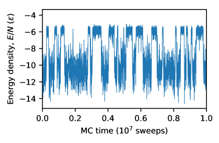
Figure 2: MC evolution of the energy density $E/N$ in a run with $N=640$, $T\approx T^{(N)}_{\mathrm{b}}$ and $\rho_{\mathrm{b}}=0.025b^{-3}$, for sequence A. Low and high energies correspond to states with and without a droplet, respectively. During the course of the run, droplet formation and dissolution occur several times.

III.1 Overall characterization

At high temperatures, the simulated systems are in a disordered state, with only small clusters present ($\lesssim 10$ chains). As the temperature is reduced, markedly larger clusters, or droplets, appear. Their formation sets in abruptly, in a narrow temperature interval, where states both with and without droplets are observed. Figure 3 shows representative snapshots of configurations with droplets for both sequences, from simulations with 640 chains. For sequence A, a single large droplet can be seen, in a dilute background with only small clusters. For sequence B, more than one droplet is often present, and the droplets are smaller than those formed by sequence A. A single large droplet is what one expects to observe if droplet formation occurs through phase separation Binder and Kalos (1980); Biskup et al. (2002); Binder (2003).

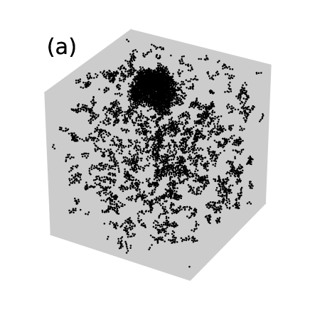
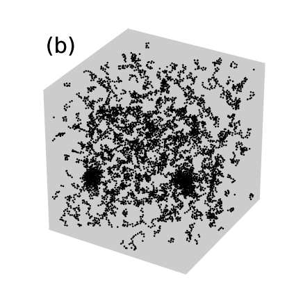
Figure 3: Snapshots showing representative droplet-containing configurations from simulations near the temperature at which droplet formation sets in, for $N=640$ and $\rho_{\mathrm{b}}=0.025b^{-3}$. Each bead is shown as a dot. (a) Sequence A, for which a single large droplet is observed. (b) Sequence B, which typically forms a few smaller droplets.

If phase separation occurs, the onset of droplet formation is, furthermore, expected to be associated with a divergence in the specific heat (Sec. II.3). Consistent with this, for sequence A, specific heat data from simulations with 10–640 chains show a peak that steadily gets higher and narrower with increasing system size [Fig. 4(a)]. The corresponding data for sequence B follow the same trend for small systems [Fig. 4(b)]. However, for this sequence, at some system size (around 80 chains), the specific heat stops growing higher and becomes multimodal. This behavior reflects the fact that sequence B forms more than one droplet in the larger systems (Fig. 3), and implies that this sequence does not undergo LLPS.

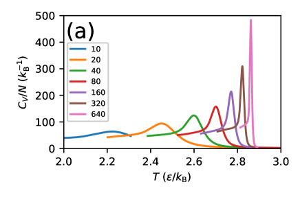
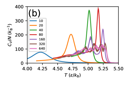
Figure 4: Temperature dependence of the specific heat, $C_{V}/N$, from simulations with 10–640 chains for fixed $\rho_{\mathrm{b}}=0.025b^{-3}$. The curves are computed by reweighting methods Ferrenberg and Swendsen (1989), using data from canonical MC simulations at several temperatures. Shaded bands indicate statistical uncertainties, but are in many cases too narrow to be visible. (a) For sequence A, the specific heat exhibits a single peak that steadily gets higher and narrower with increasing system size. (b) For sequence B, the same trend is observed but only for small systems. In the larger systems, sequence B forms more than one droplet, which leads to a multimodal specific heat.

III.2 Finite-size scaling analysis

The above results indicate that, unlike sequence B, sequence A may undergo LLPS. To determine whether or not this is the case, we next compare simulation data for several quantities with predictions from finite-size scaling theory (Sec. II.3), focusing on sequence A.

At the onset of droplet formation, due to the coexistence of states with and without a droplet, the probability distribution of energy should be bimodal, as it is at a regular temperature-driven first-order phase transition. In the latter case, the energy gap between the two phases scales linearly with system size, corresponding to a non-zero specific latent heat. However, at the droplet transition, the energy gap $\Delta E$ should scale as the critical droplet volume, or $\Delta E\sim N^{3/4}$ [Eq. (3)]. Figure 5 shows the probability distribution of the shifted and rescaled energy $\tilde{E}=(E+a)/N^{3/4}$, where $a$ is a parameter independent of $E$, for $T\approx T^{(N)}_{\mathrm{b}}$ and $\rho_{\mathrm{b}}=0.025b^{-3}$, for our three largest systems. With larger system size, the probability distribution of $\tilde{E}$ becomes increasingly bimodal in character, due to a stronger suppression of intermediate energies. By contrast, the gap between the two peaks in $\tilde{E}$ stays essentially unchanged, in perfect agreement with the predicted scaling of $\Delta E$ [Eq. (3)].

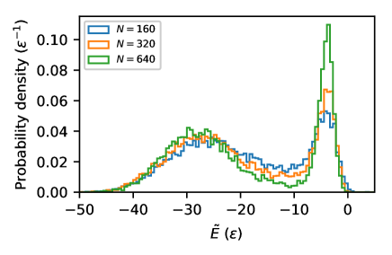
Figure 5: Probability distribution of the shifted and rescaled energy $\tilde{E}=(E+a)/N^{3/4}$ (with $a=5N\epsilon$) from simulations with 160, 320 and 640 chains for sequence A, at $T\approx T^{(N)}_{\mathrm{b}}$ and $\rho_{\mathrm{b}}=0.025b^{-3}$. Consistent with the predicted scaling relation $\Delta E\sim N^{3/4}$ [Eq. (3)], the gap between the two peaks in $\tilde{E}$ stays essentially constant, whereas the statistical suppression of intermediate energies gets stronger with increasing system size.

Assuming this scaling of $\Delta E$ with $N$ [Eq. (3)], the maximum specific heat, $C_{V,\max}/N$, should scale as $N^{1/2}$ [Eq. (5)]. Figure 6(a) shows $C_{V,\max}/N$ data against $N$ in a log-log plot, for three bead densities $\rho_{\mathrm{b}}$. Not surprisingly, the data for small systems do not follow the predicted scaling relation for large $N$. However, the data for the four largest systems ($N=80$–640) match well with the predicted form for all three bead densities.

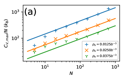
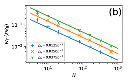
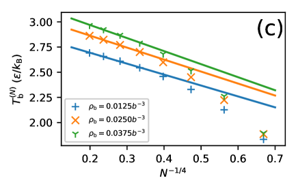
Figure 6: Finite-size scaling analysis at three bead densities $\rho_{\mathrm{b}}$ ($0.0125b^{-3}$, $0.0250b^{-3}$, $0.0375b^{-3}$) for sequence A, using data from simulations with 5–640 chains. Lines represent fits of predicted scaling expressions from Sec. II.3 to data for the four largest system sizes. (a) Log-log plot of the maximum specific heat, $C_{V,\max}/N$, against $N$. The lines are fits of the form $C_{V,\max}/N\sim N^{1/2}$ [Eq. (5)]. (b) Log-log plot of the finite-size smearing of the transition, $w_{T}$, against $N$, where $w_{T}$ is computed as the length of the temperature interval over which $C_{V}>0.8C_{V,\max}$. The lines are fits of the form $w_{T}\sim N^{-3/4}$ [Eq. (4)]. (c) The transition temperature $T^{(N)}_{\mathrm{b}}$ plotted as a function of $N^{-1/4}$. The lines are fits of the form $T^{(N)}_{\mathrm{b}}=T_{\mathrm{b}}+cN^{-1/4}$ [Eq. (2)], with $c$ and the transition temperature for infinite system size, $T_{\mathrm{b}}$, as fit parameters. The fitted values of $T_{\mathrm{b}}$ are $T_{\mathrm{b}}k_{\mathrm{B}}/\epsilon=2.92,3.10$ and 3.23 for $\rho_{\mathrm{b}}b^{3}=0.0125,0.025$ and 0.0375, respectively.

Figure 6 also illustrates the finite-size smearing and shift of the transition, for the same three bead densities. The smearing $w_{T}$ is expected to scale inversely proportional to the energy gap $\Delta E$, or $w_{T}\sim N^{-3/4}$ [Eq. (4)]. From the log-log plot in Fig. 6(b), it can be seen that the data for $w_{T}$ indeed are consistent with the predicted scaling for large $N$.

The finite-size shift of the transition temperature, $T^{(N)}_{\mathrm{b}}-T_{\mathrm{b}}$, is predicted to scale as $N^{-1/4}$ [Eq. (2)]. Therefore, Fig. 6(c) shows the data for $T^{(N)}_{\mathrm{b}}$ plotted against $N^{-1/4}$. As can be seen from this figure, fits of the form $T^{(N)}_{\mathrm{b}}=T_{\mathrm{b}}+cN^{-1/4}$, with $T_{\mathrm{b}}$ and $c$ as parameters, indeed provide a good description of the large-$N$ data ($80\leq N\leq 640$). It is worth noting that the scaling of the shift as $N^{-1/4}$, or inversely proportional to the linear size of the critical droplet, implies a slow convergence of $T^{(N)}_{\mathrm{b}}$ toward $T_{\mathrm{b}}$ with increasing $N$. In fact, for our largest systems with 640 chains, $T^{(N)}_{\mathrm{b}}$ is still about $8\%$ smaller than the fitted value of $T_{\mathrm{b}}$.

To summarize the above analysis, for all properties studied, we find that the simulation data for sequence A are consistent with the theoretical predictions, which provides strong evidence that this sequence indeed undergoes LLPS.

III.3 Droplet size and structure

The specific heat data discussed in Secs. III.1 and III.2 show that the sequences A and B, despite sharing the same length and composition, have different phase behaviors. To understand this difference, we next examine some basic structural properties of the droplets formed by these sequences. Throughout this section, we focus on data obtained using $N=640$, $\rho_{\mathrm{b}}=0.025b^{-3}$ and a temperature near the onset of droplet formation.

One important characteristic is the mass of the droplets, or the number of chains that they contain. It was already noted that sequence A forms more massive droplets than sequence B (Fig. 3). To quantify this assertion, Fig. 7 shows cluster mass distributions for both sequences. From this figure, it can be seen that, in these systems, a typical sequence A droplet accommodates about 200 chains, whereas the corresponding number for sequence B is less than 50. Also worth noting is the statistical suppression of intermediate-mass clusters, which is particularly pronounced for sequence A. If phase separation occurs, one expects to observe a single dominant droplet Binder and Kalos (1980); Biskup et al. (2002); Binder (2003), as is the case for sequence A.

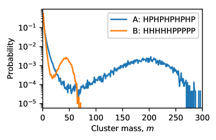
Figure 7: Mass fraction of clusters with $m$ chains, $P(m)$, as obtained using $N=640$, $\rho_{\mathrm{b}}=0.025b^{-3}$ and a temperature near the onset of droplet formation. Alternatively expressed, $P(m)$ is the probability that a randomly selected chain belongs to a cluster with $m$ chains. Sequence A forms droplets containing roughly 200 of the 640 chains, whereas intermediate-mass clusters are statistically suppressed.

Another basic characteristic is the density of the droplets. Figure 8 shows average bead density profiles around the center of mass of large clusters. Here, a given cluster is defined as large if the number of chains exceeds a threshold (75 for sequence A and 20 for sequence B), and the density is calculated as a function of the distance from its center of mass, $r_{\mathrm{cm}}$, counting all beads, whether or not they belong to a chain in the cluster. The total density is split into H and P densities. The calculated density profiles for sequence A are essentially flat at both small and large $r_{\mathrm{cm}}$ [Fig. 8(a)], suggesting that these densities are representative for the interior of droplets and the dilute background, respectively. Using this property, we find that the density inside droplets is more than a factor 40 higher than that of the dilute background (where the total bead density is $0.019b^{-3}$). Note also that the droplets are homogeneous in composition; the H to P ratio is virtually independent of $r_{\mathrm{cm}}$.

The droplets formed by sequence B exhibit, by contrast, a micellar structure, with a high-density core composed almost exclusively of H beads and a corona of mainly P beads [Fig. 8(b)]. The formation of a hydrophobic core is possible due to the block structure of this sequence. However, as the sequence is short and contains a stretch of P beads, this core can only accommodate a small number of chains, which explains the low mass of droplets formed by this sequence (Fig. 7). The mechanisms of micelle formation by block copolymers have been extensively studied by both theory and simulation Leibler et al. (1983); Nagarajan and Ganesh (1989); Milchev et al. (2001).

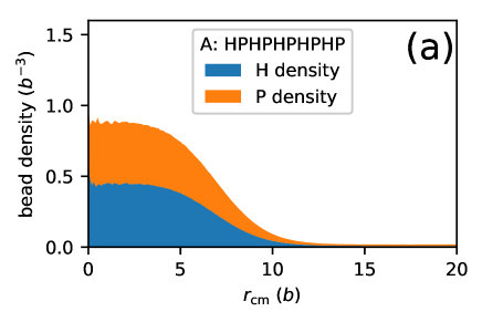
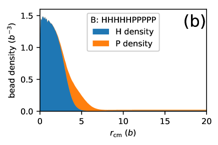
Figure 8: Bead density profiles calculated as a function of the distance $r_{\mathrm{cm}}$ from the center of mass of large clusters, for (a) sequence A and (b) sequence B. The data was obtained using $N=640$, $\rho_{\mathrm{b}}=0.025b^{-3}$ and a temperature near the onset of droplet formation. A cluster is defined as large if the number of chains is above a cutoff (75 and 20 for sequences A and B, respectively). The total density is split into H and P densities. For comparison, a perfect close-packing of the beads would give a total density of $3.35b^{-3}$.

While we have seen above that sequence A phase separates, it is still not immediately clear whether the dense phase is liquid-like. Therefore, we end with a brief assessment of the mobility of the chains in droplets formed by this sequence. The analysis uses configurations stored at a time interval of $10^{3}$ MC cycles, which is much shorter than the average droplet lifetime of about $2\cdot 10^{5}$ MC cycles. As before, a droplet is a cluster with more than 75 chains. We first consider the exchange of chains between droplets and their surroundings. To this end, whenever two consecutive snapshots both contain droplets, the chain contents of the droplets are compared. Over this timescale ($10^{3}$ MC cycles), it turns out that, on average, 44% of the chains present in the original droplet are lost, indicating a fast exchange with the surroundings compared to the lifetime of a droplet.

To get a measure of whether also the internal structure of a droplet is dynamic, we monitor changes in chain-chain contacts within droplets. To this end, given a droplet-containing snapshot, we identify all pairs of chains in the droplet that are in contact (interaction energy $<$0), and where each chain also interacts with at least 15 other chains. The latter condition serves to focus the analysis on chain pairs buried in the interior of the droplet. Whenever a droplet is present also in the next snapshot ($10^{3}$ MC cycles later), we check the fate of the contacts identified in the first snapshot. On average, we find that $54\%$ of the pairs remain in contact, whereas only about 11% are broken due to at least one of the chains leaving the droplet. This leaves 34% of the pairs separating due to internal rearrangements of the droplet, showing that the internal structure is far from rigid. Thus, the droplets are dynamic with respect to both exchange with the surroundings and their internal organization.

IV Discussion and Conclusions

It is well-known that finite-size scaling theory provides a powerful tool for analyzing phase transitions in spin models as well as vapor-to-droplet transitions in simple liquids. In this manuscript, we have applied these ideas to investigate the sequence-dependent phase behavior of a simple explicit-chain model for protein droplet formation.

Of the two specific sequences studied, the block sequence B turned out not to undergo LLPS. It is worth noting that from data for small systems, one may be led to the opposite conclusion. In particular, the observed peak in the specific heat is for small systems higher for sequence B than it is for the alternating sequence A, which does phase separate. However, above some system size (about 80 chains), the maximum specific heat does not increase further for sequence B, in contrast to what is observed for sequence A and to what one expects if phase separation takes place.

For sequence B, we observed micelle formation, rather than the formation of a droplet of a dense bulk phase. Micelle formation was found to set in at a $kT$ of about 5. Note that the system need not remain micellar in character well below this temperature. In particular, it is conceivable that the global free-energy minimum of this system contains bilayer structures at low temperatures. However, a proper investigation of the low-temperature phase structure is computationally challenging and beyond the scope of the present article.

To determine whether or not sequence A phase separates, simulation data for several properties and a range of system sizes were compared with predictions from finite-size scaling theory. In this way, the phase behavior can, in principle, be investigated in a systematic fashion, but it must be remembered that the theoretical results are leading-order predictions for large systems and therefore not necessarily valid for the system sizes amenable to simulation. It turned out, however, that a scaling behavior consistent with the predicted asymptotic one could be observed for all properties studied. Hence, taken together, the results of this analysis leave little doubt that sequence A does indeed phase separate.

It is worth noting that sequences with alternating hydrophobic and polar residues tend to have a high $\beta$-sheet propensity West et al. (1999); Hung et al. (2017). The biophysical model used in our present calculations cannot describe $\beta$-sheet formation, due to the lack of hydrogen bonding. However, it has been shown that droplet formation through LLPS sometimes is followed by maturation into a solid-like state containing amyloid fibrils Patel et al. (2015). In this case, LLPS represents a first step toward $\beta$-sheet formation.

Among the specific scaling relations studied, the finite-size shift of the transition temperature deserves special attention. This shift scales inversely proportional to the linear size, rather than the volume, of the critical droplet, so that $T^{(N)}_{\mathrm{b}}-T_{\mathrm{b}}\sim N^{-1/4}$ [Eq. (2)]. This slow convergence of the transition temperature $T^{(N)}_{\mathrm{b}}$ toward its value for infinite system size, $T_{\mathrm{b}}$, makes finite-size scaling analysis an important ingredient when determining the phase diagram from simulation data. This conclusion is highlighted by the magnitude of the relative shift of the transition temperature for sequence A, which was found to still be $\sim$8% for the largest systems with 640 chains.

Simulation methods, based on explicit-chain or field-theory representations, offer some distinct advantages over mean-field methods in the study of sequence-dependent biomolecular phase separation. However, to exploit the full potential of the simulations, the system-size dependence of the generated data needs to be understood and accounted for. The results presented here demonstrate that a systematic analysis of the system-size dependence can be both feasible and rewarding.