Fermi surfaces of composite fermions

Abstract

The fractional quantum Hall (FQH) effect was discovered in two-dimensional electron systems subject to a large perpendicular magnetic field nearly four decades ago. It helped launch the field of topological phases, and in addition, because of the quenching of the kinetic energy, gave new meaning to the phrase “correlated matter”. Most FQH phases are gapped like insulators and superconductors; however, a small subset with even denominator fractional fillings $\nu$ of the Landau level, typified by $\nu=1/2$, are found to be gapless, with a Fermi surface akin to metals. We discuss our results, obtained numerically using the infinite-Density Matrix Renormalization Group (iDMRG) scheme, on the effect of non-isotropic distortions with discrete $N$-fold rotational symmetry of the Fermi surface at zero magnetic field on the Fermi surface of the correlated $\nu=1/2$ state. We find that while the response for $N=2$ (elliptical) distortions is significant (and in agreement with experimental observations with no adjustable parameters), it decreases very rapidly as $N$ is increased. Other anomalies, like resilience to breaking the Fermi surface into disjoint pieces, are also found. This highlights the difference between Fermi surfaces formed from the kinetic energy, and those formed of purely potential energy terms in the Hamiltonian.

1 Introduction

Following the experimental discovery Tsui1982 of the FQH effect at an electron density corresponding to a filling of $\nu=1/3$ in the lowest Landau level, Laughlin Laughlin1983 provided an understanding of the existence of FQH liquid phases at other inverse odd-integer fillings, e.g. 1/5, 1/7 etc. Theoretical work Haldane1983  Jain1989  Jain2007 categorized the large number of FQH phases seen in subsequent experiments Du1993  Stormer1999 into a hierarchy of fractions. The most widely used scheme today Jain2007 relies on the concept of “composite fermions” (CFs), i.e. electrons bound to an even number of flux quanta or vortices. A mean-field description of the electron system at $\nu=1/2$ in terms of composite fermions made up of electrons bound to two flux quanta gives rise to a Fermi liquid-like state Halperin1993 known as the composite Fermi liquid (CFL). This result has been verified in a number of experiments including direct determination of the Fermi surface Kamburov2012B . Nevertheless, it is is a very counterintuitive result in terms of the original electron system for which the kinetic energy is totally quenched by Landau quantization, and the Hamiltonian consists of purely potential terms! For systems possessing continuous rotational symmetry in two dimensions, the composite Fermi surface is a circle, as might be expected, with a radius determined by Luttinger’s theorem.

It has been recognized in recent years Son2015 that this composite Fermi surface is characterized by an unusual Berry phase, which may point to the composite fermions being massless Dirac particles, and was subsequently verified numerically with various methods Geraedts2016  Geraedts2018 . Here, we consider a different, but equally interesting property of the composite fermion Fermi surface, namely its response to terms in the Hamiltonian that break rotational symmetry. This explores the geometric degree of freedom of quantum Hall states Haldane2011 .

Energy bands in solids depend significantly on the atomic structure of the constituents through the lattice symmetry and the effective pseudopotentials; consequently, Fermi surfaces of metals show tremendous variety. Deducing them using various experimental probes was a major area of study in the 1960s, which proved crucial to determine the validity of different theoretical approximations for calculating energy bands. While the alkali metals have a nearly spherical surface with small distortions, and the noble metals have spherical Fermi surfaces with multiple necks, others can be quite complex. Fig. 1, taken from Ref. Ketterson1967 , depicts the Fermi surface of solid Magnesium, with colorful descriptions of various parts – monster, cap, cigar, butterfly etc.. For another complex Fermi surface, see Ref. Ashcroft1976 .

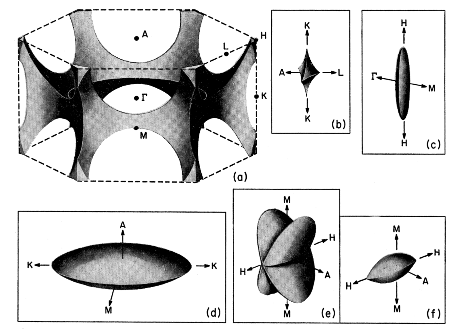
Figure 1: Fermi surfaces of solid Magnesium. From Ref. Ketterson1967 .

Given the extreme variability of Fermi surfaces of various metallic materials to atomic potentials and lattice structure, it is natural to ask how the circular Fermi surface of the correlated $\nu=1/2$ state for isotropic systems responds to terms in the Hamiltonian that do not preserve rotational symmetry. In particular, we investigated the effect of having a discrete $N$-fold symmetry in the zero-field kinetic energy, which could arise as a result of lattice symmetry, on the shape of the Fermi surface at high magnetic field at $\nu=1/2$. Surprisingly, while we found the Fermi surface distorts easily from a circular to an elliptical shape (in a manner that was quantitatively in agreement with experiments on strained GaAs quantum wells Jo2017 , see Fig. 2), other types of distortions elicited a much more subtle response. Thus, as we show analytically, the composite fermion Fermi surface is completely insensitive to isotropic distortions, even when these may split the zero-field Fermi sea into disconnected ring-shaped pieces. In an anisotropic situation, even when the zero-field Fermi surface splits into well-separated Fermi pockets, we found that the composite Fermi surface remains a single connected piece, a result also found in experiment. Kamburov2014 Finally, we found the composite Fermi surface to be extremely resilient to distortions with four-fold and higher rotational symmetry.

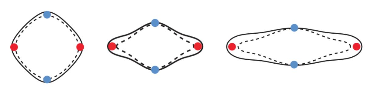
Figure 2: Fermi surfaces of holes in strained GaAs. Solid and dashed lines represent calculated values for different spin components. Dots represent results obtained from experimentally measured oscillations in the resistivity as a result of commensuration effects. From Ref. Jo2017 .

2 Mapping the Fermi contour of composite fermions

We now describe how to map the Fermi contour of composite fermions numerically with the infinite density matrix renormalization group (iDMRG) method Schollwock2011 . This method, originally developed for one-dimensional spin chains, has been successfully applied to the fractional quantum Hall problem Zaletel2013  Zaletel2015 . By placing the system on a cylinder, Landau orbitals wrapping around the finite circumference $L$ can be mapped onto sites of an infinite spin chain. This geometry is crucial to the method we are about to outline. Beyond the finite circumference $L$, DMRG naturally introduces a second cutoff, known as the bond dimension $\chi$. This is the size of the matrices used in the variational ansatz for the many body ground state, and can be thought of as a limit on the amount of quantum entanglement in the state. For gapped ground states (whose entanglement obeys an area law, i.e. it stays finite even on the infinite cylinder), the error induced by this approximation drops quickly with $\chi$ Verstraete2006 , so in principle there exists a value $\chi^{\ast}$ above which convergence within any predefined error bar is achieved. This is not true of gapless ground states, where the entanglement diverges logarithmically. As a result, this method may appear ill-suited to the study of the CFL. However, as we shall see shortly, that is not the case.

The method we use, pioneered in Ref. Geraedts2016 , relies on the static guiding center structure factor,

$$S(\mathbf{q})\equiv\langle\bar{\rho}_{\mathbf{q}}\bar{\rho}_{-\mathbf{q}}\rangle\;,$$ (1)

where $\bar{\rho}_{\mathbf{q}}\equiv\sum_{j}e^{i\mathbf{q}\cdot\mathbf{R}_{j}}$ is the LLL-projected density operator, expressed in terms of the guiding center operators $\mathbf{R}_{j}$ ($j$ labels the electrons in the system). This quantity plays a crucial role in various aspects of quantum Hall physics, e.g., the incompressibilty of FQH fluids is manifested in the long-wavelength scaling $S(q)\sim q^{4}$ Girvin1985 . In the CFL state, which is compressible, $S(\mathbf{q})$ is not expected to exhibit such quartic behavior. On the other hand, it displays a singular feature at $q=2k_{F}$, where $k_{F}$ the Fermi wavevector of composite fermions. These singularities allow us to map the Fermi contour of CFs.

By taking the $x$ axis parallel to the cylinder axis and $y$ around the finite circumference, the component $q_{y}$ is discretized in steps of $\kappa\equiv 2\pi/L$, while $q_{x}$ can in principle take on continuous values. Therefore at any finite $L$ the CF Fermi sea consists of a sequence of one-dimensional segments of lengths $\{Q_{n}\}$. The Fermi contour then consists of the isolated endpoints of such segments, $\{\mathbf{q}=\left(\pm Q_{n}/2,\kappa(n+\delta)\right)\}$.  $S(\mathbf{q})$ is expected to show a non-analytical feature whenever $\mathbf{q}$ connects two different points belonging to the Fermi contour. Locating these singularities allows us to extract the $Q_{n}$ momenta and effectively map the Fermi contour by “connecting the dots”. An example of this procedure is shown in Fig. 3. The ellipse in Fig. 3(a) represents the anisotropic Fermi sea whose shape we want to determine. The colored arrows represent vectors $\Delta\mathbf{q}$ connecting points on the Fermi contour. If we fix $\Delta q_{y}=0$ (horizontal arrows), we expect singularities in $S(\Delta q_{x},0)$ at $\Delta q_{x}=Q_{m}$. Such singularities are indeed visible in the data of Fig. 3(b), and are in principle all we need to extract the $\{Q_{n}\}$ values and map the Fermi contour. However, as a consistency check, we also find singularities at other values of $\delta q_{y}$, corresponding to vectors with a non-zero vertical component: $\Delta\mathbf{q}=\left((Q_{m}\pm Q_{n})/2,\kappa(m-n)\right)$, for $m\neq n$. A given estimate of the singularities $\{Q_{m}\}$ at $\Delta q_{y}=0$ naturally comes with a prediction for the whole set of singularities at $|\Delta q_{y}|>0$, which provides a robust test of the existence of the Fermi contour.

Since the states obtained by DMRG are approximations of the true ground state, these singularities will not be reproduced perfectly. In particular, the finite bond dimension $\chi$ introduces a finite correlation length $\xi$ (whereas the “true” CFL ground state should have algebraic correlations). As a result, the singular features in $S(\mathbf{q})$ acquire finite width $\delta q\sim\xi^{-1}$. In practice, for the sizes we study, $\delta q$ can be made small enough with $\chi\leq 6000$ that the gapless nature of the CFL is not the dominant source of uncertainty of the method.

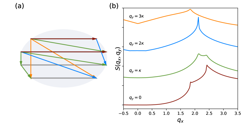
Figure 3: Mapping the CFL Fermi contour from the guiding center structure factor $S(\mathbf{q})$. (a) Fermi sea for the composite fermions at $L=17\ell_{B}$ and $\alpha_{F}=0.445$. The shaded area represents the 2D Fermi sea in the planar ($L\to\infty$) limit. The gray lines contain allowed values of $\mathbf{q}$ on the cylinder with finite $L$. Colored arrows show momenta connecting points on the Fermi contour. (b) Numerical data for $S(\mathbf{q})$ at $q_{y}=n\kappa$, $0\leq n\leq 3$, with bond dimension $\chi=3000$, translated vertically for clarity. The location of the singularities in (b) can be used to reconstruct the shape in (a), initially not known. The CF anisotropy in this case is found to be $\alpha_{CF}=0.667$.

3 Band mass anisotropy

With the method outlined above, we can test the effects of an anisotropic band mass in the kinetic energy of the zero-field carriers,

$$H_{0}=\frac{p_{x}^{2}}{2m_{xx}}+\frac{p_{y}^{2}}{2m_{yy}}\equiv\frac{1}{2m}\left(\alpha_{F}p_{x}^{2}+\alpha_{F}^{-1}p_{y}^{2}\right)\;,$$ (2)

where $m=\sqrt{m_{xx}m_{yy}}$ and $\alpha_{F}$ is the anisotropy parameter, equal to the ratio of extremal Fermi wavevectors, i.e. the square root of mass anisotropy,

$$\alpha_{F}=\frac{k_{F,y}}{k_{F,x}}=\sqrt{\frac{m_{yy}}{m_{xx}}}\;.$$ (3)

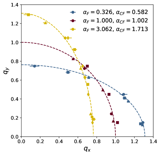
Figure 4: Location of the Fermi contour for three selected values of $\alpha_{F}$, extracted from data similar to that in Fig. 3. The dashed lines are the best fits of the data to ellipses of fixed area $\pi\ell_{B}^{-2}$, with the value of $\alpha_{CF}$ shown in the legend. Different symbols of the same color (circle, square, triangle and diamond) correspond to different system sizes for the same $\alpha_{F}$.

We consider values of $\alpha_{F}$ ranging from $0.16$ to $6.25$. At each value of $\alpha_{F}$, we map the Fermi contour as described earlier, using several values of $L$ (3 to 5 distinct values in the range of $13$ to $27\ell_{B}$, depending on $\alpha_{F}$). Examples representative of the cases $\alpha_{F}<1$, $\alpha_{F}=1$ and $\alpha_{F}>1$ are shown in Fig. 4. We extract $\alpha_{CF}$ from the optimal fit of the Fermi contour points to an ellipse. Though in the thermodynamic limit we expect an elliptical Fermi contour, our finite-size data necessarily deviate from it due to Luttinger’s theorem, which in our system fixes the total length of segments making up the finite-size Fermi sea to

$$\sum_{n}Q_{n}=\nu L\ell_{B}^{-2}\;.$$ (4)

This leads to an error in the anisotropy of our fitted ellipse because of the finite values of $L$, which we estimate to be of order $1-2\%$. We fit the discrete set of $(q_{x},q_{y})$ coordinates obtained through the process described above to an ellipse of area $\pi\ell_{B}^{-2}$ (which is fixed by the carrier density at half filling). From the optimal ellipse $(k/k_{CF,x})^{2}+(k/k_{CF,y})^{2}=1$, we obtain $\alpha_{CF}=k_{CF,y}/k_{CF,x}$.

In the planar limit $L\to\infty$, a $\pi/2$ rotation exchanges the major and minor axes of the elliptical Fermi surface, mapping $\alpha$ to $1/\alpha$. This implies that $\log(\alpha_{CF})$ is an odd function of $\log(\alpha_{F})$, so its Taylor expansion around the isotropic point $\alpha_{F}=\alpha_{CF}=1$ contains only odd powers:

$$\log(\alpha_{CF})=\sum_{n=0}^{\infty}c_{2n+1}(\log\alpha_{F})^{2n+1}=c_{1}\log\alpha_{F}+\mathcal{O}((\log\alpha_{F})^{3})\;.$$ (5)

We find Ippoliti2017A that the first term in this expansion, corresponding to a power law $\alpha_{CF}=(\alpha_{F})^{c_{1}}$, already provides a very good approximation to the data for Coulomb interaction, as shown in Fig. 5. A linear fit yields $c_{1}\simeq 0.49\pm 0.1$, close to a square-root dependence $\alpha_{CF}=\sqrt{\alpha_{F}}$. Remarkably, this is in very good agreement with experiments on holes in GaAs quantum wells under application of in-plane strain Jo2017 .

In order to test the universality of this result, we replace the Coulomb interaction with a dipolar interaction $V(r)\propto r^{-3}$, also shown in Fig. 5. This interaction could be realized in systems of cold atoms. Wilkin2000  Yao2013  Cooper2013 We find again that a single power law (i.e. a truncation of Eq. (5) to the first term) fits the data well, but we measure a significantly larger exponent $c_{1}=0.79\pm 0.01$. This is unambiguously different from a square root dependence. In particular it implies that $\alpha_{CF}$ is much closer to $\alpha_{F}$ (i.e. the CFL is much more anisotropic) than for the case of Coulomb interaction. Since the CFL anisotropy arises from the competition between the kinetic energy term (which has anisotropy $\alpha_{F}$) and the interaction (which is isotropic), this result means that the dipolar interaction is less effective than the Coulomb one at countering the effect of band mass anisotropy. This is intuitively reasonable: as $r^{-3}$ decays more quickly than $r^{-1}$, its effect on the shape of long-distance correlations will be weaker.

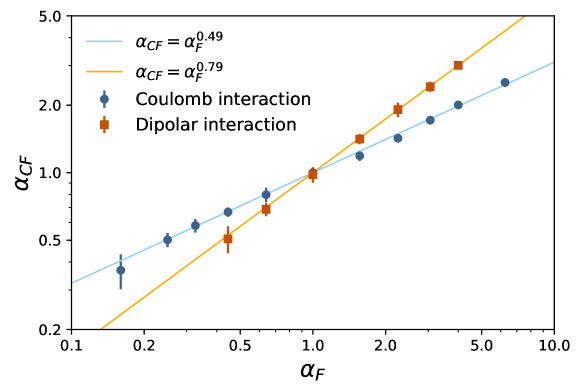
Figure 5: Composite fermion anisotropy $\alpha_{CF}$, obtained by mapping the Fermi contour of the CFL state obtained numerically with iDMRG, as a function of bare electron anisotropy $\alpha_{F}$ for Coulomb interaction $V(r)=1/r$ and dipolar interaction $V(r)=1/r^{3}$. The solid lines correspond to power-law fits $\alpha_{CF}=(\alpha_{F})^{c_{1}}$ as shown in the legend.

4 Isotropic distortions

We now take a brief departure from anisotropic deformations to consider the effect of circularly symmetric, but otherwise arbitrary, deformations of the electron dispersion Ippoliti2017B . We note in passing that non-parabolic dispersions could occur in any strongly interacting fermionic system with continuous translational and full rotational symmetry (i.e. Galilean invariance). In fact, significant deviations have been predicted and seen experimentally in Galilean invariant three-dimensional dilute mixtures of ³He in ⁴He Varma1973  Bhatt1978 which depend on the effective interaction pseudopotentials. Hsu1985

We show that the problem in the high field limit reduces to the usual Landau problem with the same extensively degenerate Landau bands (and in particular the same eigenfunctions), but with eigenvalues that generally differ from the canonical harmonic oscillator values. As a result, in the high magnetic field limit, the problem can be projected onto a single Landau level; but which one? This depends on how the nontrivial dispersion rearranges the original Landau level energies.

To get more quantitative, we consider a zero-field Hamiltonian with an arbitrary, but isotropic kinetic energy term in two dimensions:

$$H_{0}=E_{0}f\left(\frac{|\mathbf{p}|^{2}}{2mE_{0}}\right)\;,$$ (6)

where $m$ is the free electron mass, $\mathbf{p}$ is the canonical momentum, and $E_{0}$ is an arbitrary energy scale that makes the argument of $f$ dimensionless. For non-relativistic free fermions, one has $f(x)=x$ (and the energy scale $E_{0}$ cancels out). Then, the eigenstates $\{|\phi_{N,m}\rangle\}$ have eigenvalues

$$\epsilon_{N}^{\rm quadratic}=(N+1/2)\hbar\omega_{c}=(N+1/2)\beta E_{0}\;,$$ (7)

where $N$ is the Landau level index, $m$ labels the intra-LL degeneracy, $\omega_{c}=eB/m$ is the cyclotron frequency, and $\beta$ is the dimensionless ratio $\hbar\omega_{c}/E_{0}$. Since the Hamiltonian $H_{0}$ in Eq. (6) is itself a function of $|\mathbf{p}|^{2}/2m$, the $\{|\phi_{N,m}\rangle\}$ are eigenstates for any $f(x)$:

$$H_{0}|\phi_{N}\rangle=\epsilon_{N}|\phi_{N}\rangle,\quad\epsilon_{N}=E_{0}f\left((N+1/2)\beta\right)\;.$$ (8)

The simplest non-trivial example for $f(x)$ is

$$f(x)=-Cx+4x^{2}\;,$$ (9)

which gives

$$H_{0}(C)=-C\frac{|\mathbf{p}|^{2}}{2m}+\frac{1}{E_{0}}\left(\frac{|\mathbf{p}|^{2}}{m}\right)^{2}\,.$$ (10)

This kinetic energy yields a Fermi sea which is an annulus if $C>0$ and $\epsilon_{F}<0$, and a circle otherwise. The annular case can be seen as a simplified model for a realistic energy dispersion that has recently been observed Jo2017B for holes in GaAs quantum wells. It is straightforward to find values of the parameter $C$ and Fermi energy $\epsilon_{F}$ where the system has an annular Fermi sea at zero field and the $N=0$ Landau level is the one with lowest energy, giving a CFL with a circular Fermi sea. Breaking up the zero-field Fermi sea into multiple annular pieces Ippoliti2017B also yields a single, circular Fermi sea of CFs. In short, the CFL Fermi sea is completely insensitive to such isotropic distortions of the electron spectrum.

For certain choices of $f(x)$ it is also possible to have a different Landau level have minimum energy. Then, one could obtain different phases, like the Moore-Read phase Moore1991 (arising if $N=1$ has lowest energy) or symmetry-broken phases such as stripes or bubbles Moessner1996 (if $N\geq 2$ has lowest energy). This opens the exciting possibility of studying symmetry-broken phases in the extreme high-field limit, a regime opposite to the one in which they are normally observed. In the simple example of Eq. (10), we find that these phases are predicted to occur at a realistic carrier density $\sim 10^{11}{\rm cm}^{-2}$ for band parameters $C\sim 3$ and $E_{0}\sim 3{\rm meV}$. The recently observed annular Fermi sea for holes in GaAs quantum wells Jo2017B would most likely not give rise to these phases, due to the fact that the annular Fermi pocket is included in a larger Fermi sea (i.e. there is no gap between the band of interest and other bands). On the other hand, band structures that are reasonably well approximated by Eq. (10) are expected to occur quite generically in band-inverted semiconductors, such as HgTe, when a gap is opened e.g. by application of strain Moon2006 .

5 Fermi pockets

The previous Section shows that one can have an electron Fermi sea made of multiple disconnected pieces at zero field, and yet only a single CF Fermi sea at high field. We can observe a similar phenomenon for Fermi seas consisting of disconnected “pockets” without rotational symmetry, such as those shown in Fig. 6. These Fermi contours are generated from the following zero-field Hamiltonian:

$$H_{0}(\alpha)=-\left(\frac{\alpha p_{x}^{2}}{2m}+\frac{p_{y}^{2}}{2m\alpha}\right)+\frac{1}{E_{0}}\left(\frac{p_{x}^{2}+p_{y}^{2}}{m}\right)^{2}\;.$$ (11)

This is the same as Eq. (10) with $C=1$, except that we have included an anisotropy parameter $\alpha$ in the quadratic part which explicitly breaks rotational symmetry.

Fermi contours with shapes similar to those in Fig. 6 have been observed in GaAs systems in a parallel field Kamburov2014 , as well as in the surface states of Sn_1-xPb_xSe Dziawa2012 and bismuth Ohtsubo2012  Feldman2016 (though in the latter case the valleys are elongated radially, rather than tangentially). In such systems it is tempting to assume that multiple zero-field Fermi pockets imply that the system can be treated as having a single Fermi pocket and an additional “valley pseudospin” at high field. However, we will show that this assumption is not always correct.

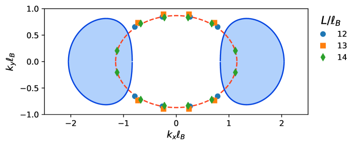
Figure 6: Fermi contour of the zero-field electrons (solid blue lines) and $\nu=1/2$ CFs (dashed red line). The latter is a fit to singularities in $S(q)$ (datapoints) obtained with iDMRG at the sizes indicated in the legend. The Hamitonian is Eq. (11) with $\alpha=4$ and the Fermi energy $\epsilon_{F}=-0.49E_{0}$. For these parameters, the inverse magnetic length at filling $\nu=1/2$ is $\ell_{B}^{-1}=0.64k_{0}$, so the two Fermi pockets are separated by $\approx 2\ell_{B}^{-1}$. Nonetheless they give a connected Fermi sea, approximately elliptical, with anisotropy $\alpha_{CF}\simeq 0.76$.

To prove this point, for the dispersion Eq. (11), we choose the Fermi energy $\epsilon_{F}$ such that there are two disconnected zero-field pockets (as in Fig. 6). Since we work at $\nu=1/2$, the Fermi energy also sets the cyclotron energy. We solve the single-particle Schrodinger equation using Eq. (11) in the strong magnetic field determined by the $\epsilon_{F}$ and $\nu$, and find the two lowest-energy Landau bands. These are even and odd under inversion, respectively, and in particular both of them have equal weight in the two valleys. When their energies become nearly degenerate (i.e., when the splitting is sufficiently smaller than the interaction strength), the interactions can pick a linear superposition the Landau band which spontaneously breaks the inversion symmetry and populates only one (randomly chosen) Fermi pocket Sodemann2017 . It would be a mistake, however, to assume that this hybridization always happens when the zero-field Fermi surface has multiple pockets. If the splitting between the two lowest-lying single-particle solutions is much larger than the strength of interactions, $\sim e^{2}/\ell_{B}\varepsilon$, then LL mixing effects are modest, and the quantum Hall problem takes place in one generalized LL that has equal weight in both valleys.

We perform iDMRG calculations on the system described by Eq. (11) placed on an infinite cylinder with circumference $L=13\ell_{B}$. We retain the lowest two generalized LLs, project the Coulomb interaction accordingly, and introduce the single-particle energy splitting. We set the total filling to be $\nu=1/2$. We obtain the many-body ground state and evaluate the difference in single-particle orbital occupations, $\delta n\equiv\langle\hat{n}_{{0}}\rangle-\langle\hat{n}_{{1}}\rangle$. We find that that the system does not valley-polarize until the interaction strength $e^{2}/\ell_{B}$ is several times larger than the inter-Landau-level gap $\delta E$. Nearly all electrons populate the inversion-even $N=0$ Landau level up to the value of $\alpha$ used in Fig. 6, where the Fermi pockets are already clearly separated. Even beyond that value, valley polarization is only possible in the immediate vicinity of isolated level crossings, or at very large values $\alpha\gtrsim 12$.

By studying the structure factor $S(\mathbf{q})$ of states with $\delta n\simeq 1/2$, at sufficiently small $\alpha$, we are able to map the Fermi contour of CFs with the method discussed previously. This shows that the composite Fermi contour goes from being a circle at the isotropic point (in agreement with the analysis of Sec. 4) to an ellipse which becomes more elongated as the parameter $\alpha$ is increased. In Fig. 6 we show the results for $\alpha=4$, where the CF Fermi contour is approximately elliptical, with a ratio of Fermi vectors $\alpha_{CF}\simeq 0.76$. Thus, we again find a lack of a simple one-to-one correspondence between the Fermi contours of zero-field electrons and CFs: while the electron Fermi sea is made of two well-separated pockets like in Fig. 6, the CFL has a Fermi sea consisting of a single connected component, close to an elliptical shape, and smoothly connected to the circular one at $\alpha=1$.

When $\alpha$ is tuned to extremely large values, we effectively have a bilayer system at total filling $\nu=1/2$, whose phase diagram may be quite complicated (and generally dependent on details of the model). In particular, gapped Halperin 331 and 113 states Halperin1983 would compete against the valley-polarized CFL. The detailed study of this problem goes beyond the scope of this work.

6 Higher-order rotational symmetry

In this Section we consider the effects of band distortions with discrete, $N$-fold rotational symmetry ($C_{N}$) Ippoliti2017C , which generalize the case of band mass anisotropy ($N=2$) studied in Sec. 3. There are generally two ways to introduce anisotropy in a quantum Hall system: either via the one-electron dispersion, or via the electron-electron interaction. In the case of elliptical ($N=2$) anisotropy, the two approaches are equivalent, since a linear coordinate transformation can move the anisotropy between the band mass tensor $m_{ab}$ and the dielectric tensor $\varepsilon_{ab}$. This is not the case for generic anisotropy, and thus band anisotropy and interaction anisotropy are not equivalent. Here we concentrate on the former. We consider a simple set of dispersions, one for each $C_{N}$ symmetry group with even $N$. Completely general distortions such as those studied in experiments can then be thought of as arising from a sum of terms with different $C_{N}$ symmetries, so the response of the CFL can be approximately broken down into its response to each individual “harmonic”.

We quantify the anisotropy by $\alpha_{F}$, defined again as the ratio of the longest and shortest Fermi wavevectors for the system at zero magnetic field, directly generalizing the definition for band mass anisotropy. The corresponding CF quantity, $\alpha_{CF}$, is defined analogously. We study a class of model dispersions $\mathcal{E}(\mathbf{k})$ that satisfy the following requirements:

1. $C_{N}$ symmetry.

2. Homogeneity: $\mathcal{E}(\mathbf{k})=k^{a}\mathcal{E}(\hat{k})$ (this guarantees the shape of the Fermi contour is independent of $\epsilon_{F}$).

3. Polynomial dependence on the components $k_{x}$, $k_{y}$ (this guarantees $\mathcal{E}$ is well-defined as an operator once the magnetic field is turned on, $\mathbf{k}\mapsto(\mathbf{p}-e\mathbf{A})/\hbar$).

4. Positivity (this guarantees $\mathcal{E}$ has a finite-energy ground state).

Functions satisfying these requirements can easily be constructed by taking the exponent $a$ to be $N$:

$$\mathcal{E}_{\lambda}(\mathbf{k})\equiv E_{0}(\ell_{0}k)^{N}(1+\lambda\cos(N\theta))\;,$$ (12)

where $(k,\theta)$ are polar coordinates in two-dimensional momentum space and $E_{0}$, $\ell_{0}$ are arbitrary units of energy and length. This clearly has the desired $C_{N}$ symmetry. Moreover, by observing that $k^{N}\cos(N\theta)=\text{Re}(ke^{i\theta})^{N}=\text{Re}(k_{x}+ik_{y})^{N}$, we see that this is a homogeneous polynomial of degree $N$ in $k_{x}$, $k_{y}$. To ensure it is bounded from below we must choose $-1<\lambda<1$. The zero field electron Fermi contour for the dispersion in Eq. (12) is given by

$$k_{F}(\theta)=\frac{A}{\ell_{0}}\left(\frac{1}{1+\lambda\cos(N\theta)}\right)^{1/N}$$ (13)

where the dimensionless prefactor is $A=(\epsilon_{F}/E_{0})^{1/N}$. The dispersions $\mathcal{E}_{-\lambda}$ and $\mathcal{E}_{\lambda}$ are related by a $\pi/N$ rotation, so we can assume $\lambda\geq 0$ without loss of generality. The anisotropy parameter $\alpha_{F}$ can be expressed in terms of $\lambda$:

$$\alpha_{F}=\frac{k_{F}(\pi/N)}{k_{F}(0)}=\left(\frac{1+\lambda}{1-\lambda}\right)^{1/N}\;.$$ (14)

While the choice of dispersion Eq. (12) is guided by simplicity, we expect it to capture the main features of realistic distortions with the given symmetry. We thus contend that our results will be generic and not particular to this special class of anisotropic dispersions.

We numerically calculate $\alpha_{CF}$ as a function of $\alpha_{F}$ for $N=4$ and 6 with the method from Sec. 2. We do so by mapping the Fermi contour $k_{CF}(\theta)$ of composite fermions as a function of the angle $\theta$. We aggregate singularities from different system sizes (three to five distinct values of the cylinder circumference ranging between $13\ell_{B}$ and $21\ell_{B}$) at the same $N$ and $\alpha_{F}$. The resulting data should satisfy Eq. (13), but with $\lambda$ replaced by a modified $\lambda_{CF}$, from which $\alpha_{CF}$ can be derived using Eq. (14).

We find that the dependence of $\alpha_{CF}$ on $\alpha_{F}$ gets much weaker as $N$ is increased. While the results for $N=2$ in Sec. 3 suggested $\alpha_{CF}\approx\alpha_{F}^{0.5}$, in this case we consistently find $\alpha_{CF}$ to be very close to 1 for $N=4$ and 6. In particular, the data for $N=4$ deviates from a power law, possibly saturating at $\alpha_{CF}\simeq 1.05$. For $N=6$ the data is entirely consistent with $\alpha_{CF}=1$ within numerical uncertainty. The results are summarized in Fig. 7. The CF Fermi contour (thin orange line) for $N=6$ is not distinguishable from a circle (dark blue dots), whereas for $N=4$ there is a small but systematic difference, visible upon close examination. This illustrates the drastic reduction in the magnitude of the effect when going from $N=2$ to $N=4$ and then $N=6$.

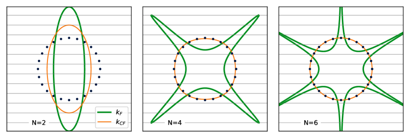
Figure 7: Fermi contours for the electrons (thick green) and the CFs (thin orange), for different values of $N$, for the same value of zero-field Fermi contour anisotropy, $\alpha_{F}=4$. The dark blue dots correspond to a circular (isotropic) Fermi contour for reference. The gray lines indicate the accessible momenta on a cylinder of circumference $L_{y}=20\ell_{B}$.

7 Discussion

We have investigated the connection between the Fermi contours of zero-field carriers (electrons or holes) and their high-field CF counterparts. We divided our analysis into four cases of interest: band mass anisotropy, which is of direct experimental interest; isotropic zero-field dispersions, potentially giving rise to a Fermi sea consisting of one or more annuli; anisotropic dispersions giving rise to multiple disconnected pockets; and anisotropic dispersions with higher-order discrete rotational symmetry ($C_{N}$ with $N>2$).

In general, we find the effects on the CFL to be quite subtle. An exact analytical argument allows us to prove that the CFL is completely insensitive to the rotationally-symmetric distortion, so that its Fermi contour remains a circle, regardless of whether the system at zero field develops a disconnected Fermi sea. A similar conclusion extends to the many-valley case, where the CFL either has a single connected Fermi sea, or may transition into different phases, depending on the separation of the pockets and the magnetic field. In the case of higher-order rotational symmetry, while we do observe transference of the $C_{4}$-symmetric anisotropy to the CFL, the magnitude of the effect is very small. For $N\geq 6$ the effect is smaller than our numerical accuracy, and thus most likely not measurable in experiment.

The model bands we have used to study the effects of $C_{N}$ symmetry were designed ad hoc and as such may be unrealistic. In particular, the absence of $k^{2}$ terms for $N>2$ is non-generic. However, restoring such isotropic terms would make the problem less anisotropic overall. Thus our model bands capture the essential features of distortions with the given symmetry, and a bound on their effect directly implies a bound on the effect of more realistic dispersions. Our results show that the quadrupolar ($N=2$) distortion, corresponding to band mass anisotropy, has by far the strongest effect, with the effect of higher angular numbers decaying rapidly. This indicates that finer structures in the zero-field problem are more efficiently washed out at high field. This is a consequence of Landau-level projection (quantifiable by decomposing the projected Hamiltonian into anisotropic pseudopotentials Ippoliti2017C  BoYang2017A ), and is thus not exclusive to the CFL state. Indeed, similar behavior is observed (through a different diagnostic) in incompressible states Krishna2019 .

We conclude by mentioning recent work Leaw2019 that finds a universal Fermi contour anisotropy renormalization in two-dimensional, Coulomb-interacting Dirac systems. The result is seemingly consistent with the behavior of the CFL in the presence of band mass ansiotropy, $\alpha_{CF}\approx\sqrt{\alpha_{F}}$, as seen both in experiment and in our simulations. The connection between these results is unclear, as the CFs are not expected to interact via the Coulomb interaction, and their Dirac nature is not conclusively established. Either way, explaining properties of the CFL through general Fermi liquid physics is a fascinating direction for future work, even beyond the geometric distortions studied here. In particular, this may lead to a better understanding the excitation spectrum of this peculiar quantum fluid.

- (1) D.C. Tsui, H.L. Stormer, A.C. Gossard, Two-dimensional magnetotransport in the extreme quantum limit, Phys. Rev. Lett. 48, 1559 (1982). DOI 10.1103/PhysRevLett.48.1559. URL https://link.aps.org/doi/10.1103/PhysRevLett.48.1559
- (2) R.B. Laughlin, Anomalous quantum Hall effect: An incompressible quantum fluid with fractionally charged excitations, Phys. Rev. Lett. 50, 1395 (1983). DOI 10.1103/PhysRevLett.50.1395. URL https://link.aps.org/doi/10.1103/PhysRevLett.50.1395
- (3) F.D.M. Haldane, Fractional quantization of the Hall effect: A hierarchy of incompressible quantum fluid states, Phys. Rev. Lett. 51, 605 (1983). DOI 10.1103/PhysRevLett.51.605. URL https://link.aps.org/doi/10.1103/PhysRevLett.51.605
- (4) J.K. Jain, Composite-fermion approach for the fractional quantum Hall effect, Phys. Rev. Lett. 63, 199 (1989). DOI 10.1103/PhysRevLett.63.199. URL https://link.aps.org/doi/10.1103/PhysRevLett.63.199
- (5) J.K. Jain, Composite fermions (Cambridge University Press, 2007). DOI 10.1017/CBO9780511607561
- (6) R.R. Du, H.L. Stormer, D.C. Tsui, L.N. Pfeiffer, K.W. West, Experimental evidence for new particles in the fractional quantum Hall effect, Phys. Rev. Lett. 70, 2944 (1993). DOI 10.1103/PhysRevLett.70.2944. URL https://link.aps.org/doi/10.1103/PhysRevLett.70.2944
- (7) H.L. Stormer, D.C. Tsui, A.C. Gossard, The fractional quantum Hall effect, Rev. Mod. Phys. 71, S298 (1999). DOI 10.1103/RevModPhys.71.S298. URL https://link.aps.org/doi/10.1103/RevModPhys.71.S298. – and references therein.
- (8) B.I. Halperin, P.A. Lee, N. Read, Theory of the half-filled Landau level, Phys. Rev. B 47, 7312 (1993). DOI 10.1103/PhysRevB.47.7312. URL http://link.aps.org/doi/10.1103/PhysRevB.47.7312
- (9) D. Kamburov, M. Shayegan, L.N. Pfeiffer, K.W. West, K.W. Baldwin, Commensurability oscillations of hole-flux composite fermions, Phys. Rev. Lett. 109, 236401 (2012). DOI 10.1103/PhysRevLett.109.236401. URL https://link.aps.org/doi/10.1103/PhysRevLett.109.236401
- (10) D.T. Son, Is the composite fermion a Dirac particle?, Phys. Rev. X 5, 031027 (2015). DOI 10.1103/PhysRevX.5.031027. URL http://link.aps.org/doi/10.1103/PhysRevX.5.031027
- (11) S.D. Geraedts, M.P. Zaletel, R.S.K. Mong, M.A. Metlitski, A. Vishwanath, O.I. Motrunich, The half-filled Landau level: The case for Dirac composite fermions, Science 352(6282), 197 (2016). DOI 10.1126/science.aad4302. URL http://science.sciencemag.org/content/352/6282/197
- (12) S.D. Geraedts, J. Wang, E.H. Rezayi, F.D.M. Haldane, Berry phase and model wave function in the half-filled Landau level, Phys. Rev. Lett. 121, 147202 (2018). DOI 10.1103/PhysRevLett.121.147202. URL https://link.aps.org/doi/10.1103/PhysRevLett.121.147202
- (13) F.D.M. Haldane, Geometrical description of the fractional quantum Hall effect, Phys. Rev. Lett. 107, 116801 (2011). DOI 10.1103/PhysRevLett.107.116801. URL http://link.aps.org/doi/10.1103/PhysRevLett.107.116801
- (14) J.B. Ketterson, R.W. Stark, Fermi surface of magnesium. I. Magnetoacoustic attenuation, Phys. Rev. 156, 748 (1967). DOI 10.1103/PhysRev.156.748. URL https://link.aps.org/doi/10.1103/PhysRev.156.748
- (15) N.W. Ashcroft, N.D. Mermin, Solid State Physics (Holt, Rinehart and Winston, New York, 1976). See page 306 for the complex Fermi surface of Tungsten.
- (16) I. Jo, K.A.V. Rosales, M.A. Mueed, L.N. Pfeiffer, K.W. West, K.W. Baldwin, R. Winkler, M. Padmanabhan, M. Shayegan, Transference of Fermi contour anisotropy to composite fermions, Phys. Rev. Lett. 119, 016402 (2017). DOI 10.1103/PhysRevLett.119.016402. URL https://link.aps.org/doi/10.1103/PhysRevLett.119.016402
- (17) D. Kamburov, M.A. Mueed, M. Shayegan, L.N. Pfeiffer, K.W. West, K.W. Baldwin, J.J.D. Lee, R. Winkler, Fermi contour anisotropy of gaas electron-flux composite fermions in parallel magnetic fields, Phys. Rev. B 89, 085304 (2014). DOI 10.1103/PhysRevB.89.085304. URL http://link.aps.org/doi/10.1103/PhysRevB.89.085304
- (18) U. Schollwöck, The density-matrix renormalization group, Rev. Mod. Phys. 77, 259 (2005). DOI 10.1103/RevModPhys.77.259. URL https://link.aps.org/doi/10.1103/RevModPhys.77.259
- (19) M.P. Zaletel, R.S.K. Mong, F. Pollmann, Topological characterization of fractional quantum Hall ground states from microscopic Hamiltonians, Phys. Rev. Lett. 110, 236801 (2013). DOI 10.1103/PhysRevLett.110.236801. URL http://link.aps.org/doi/10.1103/PhysRevLett.110.236801
- (20) M.P. Zaletel, R.S.K. Mong, F. Pollmann, E.H. Rezayi, Infinite density matrix renormalization group for multicomponent quantum Hall systems, Phys. Rev. B 91, 045115 (2015). DOI 10.1103/PhysRevB.91.045115. URL https://link.aps.org/doi/10.1103/PhysRevB.91.045115
- (21) F. Verstraete, J.I. Cirac, Matrix product states represent ground states faithfully, Phys. Rev. B 73, 094423 (2006). DOI 10.1103/PhysRevB.73.094423. URL https://link.aps.org/doi/10.1103/PhysRevB.73.094423
- (22) S.M. Girvin, A.H. MacDonald, P.M. Platzman, Collective-excitation gap in the fractional quantum Hall effect, Phys. Rev. Lett. 54, 581 (1985). DOI 10.1103/PhysRevLett.54.581. URL https://link.aps.org/doi/10.1103/PhysRevLett.54.581
- (23) M. Ippoliti, S.D. Geraedts, R.N. Bhatt, Numerical study of anisotropy in a composite Fermi liquid, Phys. Rev. B 95, 201104 (2017). DOI 10.1103/PhysRevB.95.201104. URL https://link.aps.org/doi/10.1103/PhysRevB.95.201104
- (24) N.K. Wilkin, J.M.F. Gunn, Condensation of “composite bosons” in a rotating BEC, Phys. Rev. Lett. 84, 6 (2000). DOI 10.1103/PhysRevLett.84.6. URL http://link.aps.org/doi/10.1103/PhysRevLett.84.6
- (25) N.Y. Yao, A.V. Gorshkov, C.R. Laumann, A.M. Läuchli, J. Ye, M.D. Lukin, Realizing fractional Chern insulators in dipolar spin systems, Phys. Rev. Lett. 110, 185302 (2013). DOI 10.1103/PhysRevLett.110.185302. URL https://link.aps.org/doi/10.1103/PhysRevLett.110.185302
- (26) N.R. Cooper, J. Dalibard, Reaching fractional quantum Hall states with optical flux lattices, Phys. Rev. Lett. 110, 185301 (2013). DOI 10.1103/PhysRevLett.110.185301. URL https://link.aps.org/doi/10.1103/PhysRevLett.110.185301
- (27) M. Ippoliti, S.D. Geraedts, R.N. Bhatt, Connection between Fermi contours of zero-field electrons and composite fermions in two-dimensional systems, Phys. Rev. B 96, 045145 (2017). DOI 10.1103/PhysRevB.96.045145. URL https://link.aps.org/doi/10.1103/PhysRevB.96.045145
- (28) C. Varma, Spectrum of 3He atoms in superfluid 4He, Physics Letters A 45(4), 301 (1973). DOI https://doi.org/10.1016/0375-9601(73)90089-3. URL http://www.sciencedirect.com/science/article/pii/0375960173900893
- (29) R.N. Bhatt, excitations in dilute mixtures with , Phys. Rev. B 18, 2108 (1978). DOI 10.1103/PhysRevB.18.2108. URL https://link.aps.org/doi/10.1103/PhysRevB.18.2108
- (30) W. Hsu, D. Pines, C.H. Aldrich, Elementary excitations in dilute mixtures of 3He in superfluid 4He, Phys. Rev. B 32, 7179 (1985). DOI 10.1103/PhysRevB.32.7179. URL https://link.aps.org/doi/10.1103/PhysRevB.32.7179
- (31) I. Jo, Y. Liu, L.N. Pfieffer, K.W. West, K.W. Baldwin, R. Winkler, M. Shayegan, Signatures of an annular Fermi sea, Phys. Rev. B 95, 035103 (2017). DOI 10.1103/PhysRevB.95.035103. URL http://link.aps.org/doi/10.1103/PhysRevB.95.035103
- (32) G. Moore, N. Read, Nonabelions in the fractional quantum Hall effect, Nuclear Physics B 360(2), 362 (1991). DOI https://doi.org/10.1016/0550-3213(91)90407-O. URL http://www.sciencedirect.com/science/article/pii/055032139190407O
- (33) R. Moessner, J.T. Chalker, Exact results for interacting electrons in high Landau levels, Phys. Rev. B 54, 5006 (1996). DOI 10.1103/PhysRevB.54.5006. URL https://link.aps.org/doi/10.1103/PhysRevB.54.5006
- (34) C.Y. Moon, S.H. Wei, Band gap of Hg chalcogenides: Symmetry-reduction-induced band-gap opening of materials with inverted band structures, Phys. Rev. B 74, 045205 (2006). DOI 10.1103/PhysRevB.74.045205. URL https://link.aps.org/doi/10.1103/PhysRevB.74.045205
- (35) P. Dziawa, B.J. Kowalski, K. Dybko, R. Buczko, A. Szczerbakow, M. Szot, E. Lusakowska, T. Balasubramanian, B.M. Wojek, M.H. Berntsen, O. Tjernberg, T. Story, Topological crystalline insulator states in Pb1-xSnxSe, Nature Materials 11, 1023 (2012). URL https://doi.org/10.1038/nmat3449
- (36) Y. Ohtsubo, J. Mauchain, J. Faure, E. Papalazarou, M. Marsi, P. Le Fèvre, F. Bertran, A. Taleb-Ibrahimi, L. Perfetti, Giant anisotropy of spin-orbit splitting at the bismuth surface, Phys. Rev. Lett. 109, 226404 (2012). DOI 10.1103/PhysRevLett.109.226404. URL http://link.aps.org/doi/10.1103/PhysRevLett.109.226404
- (37) B.E. Feldman, M.T. Randeria, A. Gyenis, F. Wu, H. Ji, R.J. Cava, A.H. MacDonald, A. Yazdani, Observation of a nematic quantum Hall liquid on the surface of bismuth, Science 354(6310), 316 (2016). DOI 10.1126/science.aag1715. URL http://science.sciencemag.org/content/354/6310/316
- (38) I. Sodemann, Z. Zhu, L. Fu, Quantum Hall ferroelectrics and nematics in multivalley systems, Phys. Rev. X 7, 041068 (2017). DOI 10.1103/PhysRevX.7.041068. URL https://link.aps.org/doi/10.1103/PhysRevX.7.041068
- (39) B.I. Halperin, Theory of the quantized Hall conductance, Helv. Phys. Acta 56, 75 (1983)
- (40) M. Ippoliti, S.D. Geraedts, R.N. Bhatt, Composite fermions in bands with -fold rotational symmetry, Phys. Rev. B 96, 115151 (2017). DOI 10.1103/PhysRevB.96.115151. URL https://link.aps.org/doi/10.1103/PhysRevB.96.115151
- (41) B. Yang, Z.X. Hu, C.H. Lee, Z. Papić, Generalized pseudopotentials for the anisotropic fractional quantum Hall effect, Phys. Rev. Lett. 118, 146403 (2017). DOI 10.1103/PhysRevLett.118.146403. URL https://link.aps.org/doi/10.1103/PhysRevLett.118.146403
- (42) A. Krishna, F. Chen, M. Ippoliti, R.N. Bhatt, Interaction-dependent anisotropy of fractional quantum Hall states, Phys. Rev. B 100, 085129 (2019). DOI 10.1103/PhysRevB.100.085129. URL https://link.aps.org/doi/10.1103/PhysRevB.100.085129
- (43) J.N. Leaw, H.K. Tang, M. Trushin, F.F. Assaad, S. Adam, Universal Fermi-surface anisotropy renormalization for interacting Dirac fermions with long-range interactions, Proceedings of the National Academy of Sciences 116(52), 26431 (2019). DOI 10.1073/pnas.1913096116. URL https://www.pnas.org/content/116/52/26431