QSO photometric redshifts from SDSS, WISE and GALEX colours

Abstract

Machine learning techniques, specifically the $k$-nearest neighbour algorithm applied to optical band colours, have had some success in predicting photometric redshifts of quasi-stellar objects (QSOs): Although the mean of differences between the spectroscopic and photometric redshifts, $\Delta z$, is close to zero, the distribution of these differences remains wide and distinctly non-Gaussian. As per our previous empirical estimate of photometric redshifts, we find that the predictions can be significantly improved by adding colours from other wavebands, namely the near-infrared and ultraviolet. Self-testing this, by using half of the 33 643 strong QSO sample to train the algorithm, results in a significantly narrower spread in $\Delta z$ for the remaining half of the sample. Using the whole QSO sample to train the algorithm, the same set of magnitudes return a similar spread in $\Delta z$ for a sample of radio sources (quasars). Although the matching coincidence is relatively low (739 of the 3663 sources having photometry in the relevant bands), this is still significantly larger than from the empirical method (2%) and thus may provide a method with which to obtain redshifts for the vast number of continuum radio sources expected to be detected with the next generation of large radio telescopes.

1 Introduction

There is currently much interest in developing reliable photometry-based redshifts for distant active galactic nuclei (Luken et al. 2019 and references therein). Much of this is driven by the large number of sources expected to be detected through continuum surveys with the next generation of telescopes, such as the Australian Square Kilometre Array Pathfinder (ASKAP, Johnston et al. 2008), the LOw-Frequency ARray (LOFAR, van Haarlem et al. 2013) and the extended Röntgen Survey with an Imaging Telescope Array (eROSITA, Salvato 2014). For example, the Evolutionary Map of the Universe (EMU, Norris et al. 2011) on the ASKAP is expected to yield 70 million radio sources. Being able to add a third coordinate, even statistically, would significantly increase the scientific value of these surveys. Obtaining the spectroscopic redshift ($z_{\rm spec}$) for each source would be impractical thus the need for “quick and easy” photometric redshifts ($z_{\rm phot}$). Furthermore, extinction by intervening dust can make optical spectroscopy difficult (Curran et al., 2006), whereas high redshift sources, sufficiently luminous to yield a reliable spectroscopic redshift, ionise all of the neutral gas within the host galaxy (Curran & Whiting, 2012; Curran et al., 2019), biasing against the detection of gas-rich objects (Morganti et al., 2015).

Ideally, the redshifts for radio sources would be obtained from the radio photometric properties, although this has proven to be elusive (Majic & Curran, 2015; Norris et al., 2019), due to their relatively featureless spectral energy distributions (SEDs). There has, however, been considerable success applying machine learning methods of optical-band magnitudes, specifically with the $k$-nearest neighbour (kNN) algorithm which compares the Euclidean distance between a datum and its $k$ nearest neighbours in a feature space (Ball et al., 2008), typically the $u-g$, $g-r$, $r-i$ and $i-z$ colours of the Sloan Digital Sky Survey (SDSS). However, as noted by Curran & Moss (2019), this method fails at $z\stackrel{{\scriptstyle>}}{{{}_{\sim}}}2$, giving a non-Gaussian (fat-tailed) distribution of $\Delta z\equiv z_{\rm spec}-z_{\rm phot}$ (Richards et al., 2001; Weinstein et al., 2004; Maddox et al., 2012; Han et al., 2016).

Finding an empirical relationship between the ratio of two colours and the redshift, Curran & Moss obtain a near-Gaussian distribution of $\Delta z$, via a redshift dependent colour ratio, the approximate redshift first being estimated from a near-infrared magnitude (see also Wang et al. 2016; Glowacki et al. 2017 and references therein). Thus, different combinations of observed-frame colours are required in order to yield a useful photometric redshift. We therefore suspect that the breakdown in the kNN method is due to the exclusive use of optical (SDSS) photometry and find that the redshift predictions can be significantly improved with the addition of photometry from other bands, which we address in this letter.

2 Analysis and results

2.1 The sample

From the SDSS Data Release 12 (DR12, Alam et al. 2015), we extracted the first 33 643 QSOs with accurate spectroscopic redshifts ($\delta z/z<0.01$), which span the magnitude range $r=14.667-22.618$. We then used the source coordinates to obtain the nearest source within a 6 arc-second search radius in the NASA/IPAC Extragalactic Database (NED), which usually resulted in a single match. As well as obtaining the specific flux densities, we used the NED names to query the Wide-Field Infrared Survey Explorer (WISE, Wright et al. 2010) and the Two Micron All Sky Survey (2MASS, Skrutskie et al. 2006) databases. For each of the bands, the photometric points which fell within $\Delta\log_{10}\nu=\pm 0.05$ of the central frequency of the band were averaged, with this then being converted to a magnitude.

2.2 QSO colours and photometric redshifts

2.2.1 SDSS colours

We start by using the standard $u-g$, $g-r$, $r-i$ and $i-z$ colours (Richards et al., 2001; Ball et al., 2008), including also the $r$ magnitude as a feature in the algorithm (Han et al., 2016). Of the sample of 33 643, 33 166 have all five SDSS magnitudes, giving a 98% matching coincidence. We trained the model on half of the sample, finding that $k\approx 10$ nearest neighbours minimised the standard deviation, $\sigma$, from the $z_{\rm phot}=z_{\rm spec}$ line (Fig. 1, top left).

In the top panel of the figure, we see a similar distribution to those obtained by Richards et al. (2001); Weinstein et al. (2004); Han et al. (2016), with two dense groups of outliers within $z_{\rm spec}\stackrel{{\scriptstyle<}}{{{}_{\sim}}}2$ and $z_{\rm phot}\stackrel{{\scriptstyle<}}{{{}_{\sim}}}2$. The data also exhibit the deviation from $z_{\rm phot}=z_{\rm spec}$ at $z_{\rm spec}\stackrel{{\scriptstyle>}}{{{}_{\sim}}}2$, contributing to the wide wings in the $\Delta z$ distribution (Richards et al. 2001; Weinstein et al. 2004; Maddox et al. 2012; Peters et al. 2015; Richards et al. 2015; Han et al. 2016; Curran & Moss 2019).

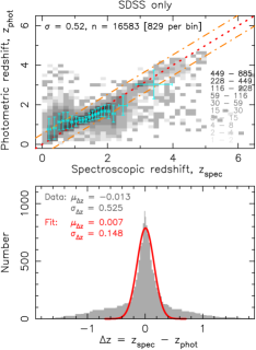
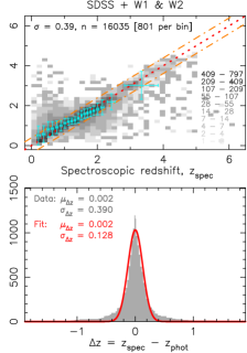
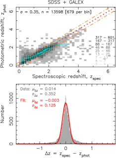
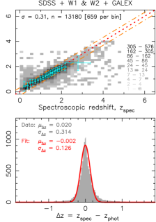
Figure 1: The results from the various models using $k=10$ nearest neighbours. The grey-scale shows the photometric versus the spectroscopic redshift, with the key to the right showing the number of sources represented. The error bars show the mean values, with the $\pm 1\sigma$ standard deviation in equally sized bins. The dotted line shows $z_{\rm phot}=z_{\rm spec}$, with the dot–dashed lines showing the standard deviation from this. The histogram below shows the $z_{\rm spec}-z_{\rm phot}$ distribution, where the mean and standard deviation is given for both the distribution and the Gaussian fit. The outlier fractions are summarised in Table 1.

2.2.2 WISE colours

As stated in Sect. 1, given the dependence of the observed-frame bands on redshift, a single set of colours would not be expected to yield accurate photometric redshifts over a wide range. Specifically, Curran & Moss (2019) find that it is the rest-frame $(U-K)/(W2-FUV)$ colour ratio which correlates strongly with redshift, corresponding to the observed-frame ratios $(I-W2)/(W3-U)$ at $1\leq z\leq 3$ and $(I-W2.5)/(W4-R)$ at $z>3$. They postulate that this dependence results from a decrease in the rest-frame $U-K$ colour coupled with an increase in the $W2-FUV$ colour as the luminosity increases, which gives a proxy for the redshift via the Malmquist bias.

It is therefore apparent that in order to accurately determine a large range of photometric redshifts, other bands beyond the optical must be invoked. The method of Curran & Moss requires nine different magnitude measures from a number of disparate surveys, resulting in photometric redshifts being obtained for $<34$% of the sources. The WISE database provides two near-infrared (NIR, $W1$ & $W2$) and two mid-infrared (MIR, $W3$ & $W4$) magnitudes from a single survey and overlaps well with the sources in the SDSS database (e.g. Lang et al. 2016; Salim et al. 2016; Wang et al. 2016). Adding the $z-W1$, $W1-W2$, $W2-W3$ and $W3-W4$ colours to the algorithm, we obtain considerably better photometric redshifts, with greatly reduced wings in the $\Delta z$ distribution (Fig. 1, top middle). Using sources for which all four WISE magnitudes are available yields a 72% matching coincidence, with the missing sources due to the objects being undetected in the $W3$ and $W4$ bands.

The matching coincidence can be increased to 95% by using the $W1$ and $W2$ magnitudes only, which returns a similar result to using all of the WISE magnitudes (Fig. 1, top right). This could be due to the $W3$ and $W4$ magnitudes probing a relatively featureless region of the SED (see Sect. 3), which does not contribute significantly to the model.

2.2.3 GALEX colours

In addition to the infrared, the ultraviolet (UV) colours may also be used to improve upon the optical data alone: Ball et al. (2008) combined the SDSS colours with the near-ultraviolet ($NUV$, $\lambda=227$ nm) and far-ultraviolet ($FUV$, $\lambda=153$ nm) bands of the Galaxy Evolution Explorer (Martin et al., 2005) to obtain a standard deviation of $\sigma=0.34$ from 11 149 QSOs. The GALEX database was also queried as part of the photometry search (Sect. 2.1) and, adding $FUV-NUV$ and $NUV-u$ to the SDSS colours in the algorithm (Fig. 1, bottom left), we obtain a similar standard deviation as Ball et al.. This is a significant improvement over the SDSS colours alone and a slight improvement over the SDSS+WISE colours. However, due to the Lyman break (see Sect. 3), the signal in the GALEX data drops significantly at high redshift, particularly at $z\stackrel{{\scriptstyle>}}{{{}_{\sim}}}3$ (see Fig. 2), which will limit the GALEX photometry’s usefulness at high redshift.

Adding the WISE to the GALEX colours (Fig. 1, bottom middle), we see further improvement although at the cost of the matching coincidence falling to 59%. As before, using the $W1$ and $W2$ magnitudes only gives a similar result while retaining a 78% coincidence (Fig. 1, bottom right).

3 Discussion

By adding the WISE to the SDSS colours in the kNN algorithm, we obtain significantly better photometric redshifts than from using the SDSS alone (cf. Richards et al. 2001; Weinstein et al. 2004; Maddox et al. 2012; Han et al. 2016). Furthermore, this is without the need to filter out outliers (red sources, e.g. Richards et al. 2001), nor the visual inspection of images prior to their inclusion in the algorithm (e.g. Maddox et al. 2012). Even just the addition of the two NIR ($W1$ & $W2$) magnitudes leads to significant improvement, which can be further enhanced with the addition of the GALEX magnitudes (Table 1).

Table 1: Summary of the algorithm performances for the SDSS sample. $n$ gives the matching coincidence of sources (out of 16 850) and is followed by the percentage of photometric redshifts which lie within $\Delta z$ of the spectroscopic value.

Algorithm	$n$	Percentage within $\Delta z$
		$\pm 0.1$	$\pm 0.2$	$\pm 0.5$
SDSS	16 583	37.1	56.4	77.4
SDSS + WISE	12 029	43.9	69.4	90.5
SDSS + $W1$ & $W2$	16 035	47.7	71.3	90.2
SDSS + GALEX	13 598	48.5	72.1	91.0
SDSS + GALEX	13 598	48.5	72.1	91.0
SDSS + $W1$ & $W2$ + GALEX	13 180	50.5	75.1	94.1

In Fig. 2 we show the mean spectral energy distributions of the sample at various redshifts, where we see the inflection at $\lambda\approx 1$ $\mu$m, as the NIR emission from heated dust transitions to the optical emission from the accretion disk (Robson 1996 and references therein).

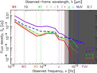
Figure 2: Mean SEDs of the SDSS sample at $z>0.2$ (29 217 photometry points), $0.95<z<1.05$ (41 383 points), $1.95<z<2.05$ (33 461 points), $2.8<z<3.2$ (16 464 points) and $3.5<z<4.5$ (14 464 points). The light grey region shows the range of the Lyman break due to $\lambda\leq 1216$ Å absorption and the dark region for $\lambda\leq 912$ Å absorption, at $z\leq 4$.

The excess at $\lambda\stackrel{{\scriptstyle>}}{{{}_{\sim}}}1$ $\mu$m from the warm dust is also apparent (e.g. Bianchini et al. 2019), although only the shape of the $JHK$ profile shows any redshift dependence. An increase in the peak frequency, which would counter the redshift of the profile, would be expected as the luminosity (redshift) increases due to the higher peak temperature of a modified blackbody (Curran & Duchesne 2019 and references therein). The addition of the NIR bands permits the inclusion of these features, explaining why the $K$ ($\lambda=2.2$ $\mu$m) and $W2$ bands are crucial to the empirical model (Curran & Moss, 2019). Another feature is the Lyman break, where UV photons are absorbed by intervening hydrogen. This is also apparent in Fig. 2, particularly for the mean $z=4$ SED, where the first drop in flux at $\lambda_{\rm rest}=0.1216$ $\mu$m ($\lambda_{\rm obs}=0.61$ $\mu$m) is due to Lyman-$\alpha$ absorption and the second drop due to ionisation by $\lambda_{\rm rest}=0.0912$ $\mu$m ($\lambda_{\rm obs}=0.46$ $\mu$m) photons. The addition of the GALEX bands permits the inclusion of this feature at low redshift, although, the steep drop in flux results in a loss of signal at high redshift. Thus, the incorporation of upper limits to the UV fluxes into the algorithm would be required in order to fully utilise this feature.

As stated in Sect. 1, a photometric redshift estimate based only upon the source magnitudes will prove invaluable to large surveys of redshifted continuum sources. Of particular interest are radio sources, in the era of the Square Kilometre Array and its pathfinders. Given that, in practice, the detections from blind radio surveys will then be checked/re-observed for photometry in other bands, we wish to test the algorithm on an independent radio selected sample which has been followed up for spectroscopic redshifts, rather than an optical sample (SDSS), which has been cross-matched with radio sources. We therefore use the Optical Characteristics of Astrometric Radio Sources (OCARS) catalogue of Very Long Baseline Interferometry astrometry sources, a sample of flat spectrum radio sources (quasars) observed over five radio bands (spanning 2–27 GHz), with $S$-band flux densities ranging from 15 mJy to 4.0 Jy (Ma et al., 2009). Of these, 3663 have spectroscopic redshifts (Malkin, 2018), with 36% having the full SDSS photometry (Table 2).

Table 2: As Table 1, but for the OCARS sample (out of 3663 sources).

Algorithm	$n$	Percentage within $\Delta z$
		$\pm 0.1$	$\pm 0.2$	$\pm 0.5$
SDSS	1320	27.1	44.4	66.9
SDSS + WISE	1007	37.3	56.2	80.6
SDSS + $W1$ & $W2$	1187	38.8	59.9	79.3
SDSS + GALEX	810	41.7	61.6	83.3
SDSS + WISE + GALEX	676	44.4	63.9	86.8
SDSS + $W1$ & $W2$ + GALEX	739	47.9	68.9	89.3

Since our aim is to predict the photometric redshifts of a radio selected sample, with no a priori knowledge of the spectroscopic redshifts, we train the algorithm on the full SDSS sample. The model is then applied to the OCARS sources with the relevant photometry, as well as spectroscopic redshifts (in order to test the results). In Fig. 3, we see different distributions than from the SDSS photometric redshifts (Fig. 1),

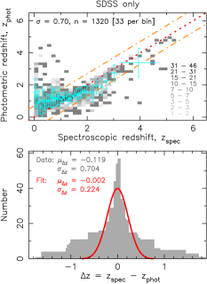
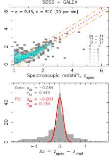
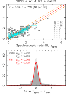
Figure 3: As Fig. 1, but using the SDSS sample to obtain the photometric redshifts of the OCARS sample.

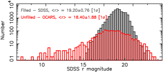
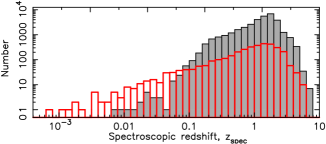
Figure 4: The $r$ band magnitudes (top) and redshift distribution (bottom) for the SDSS (filled) and OCARS (unfilled histogram) sources.

which is confirmed by the spread in magnitudes (Fig. 4, top), possibly due to the wider range of redshifts of the OCARS sample (Fig. 4, bottom). Nevertheless, training the algorithm on the SDSS sample gives photometric redshifts which are nearly as accurate as for the SDSS sources themselves (Fig. 1) when all three surveys are used (Fig. 3, right), with the percentages within $\Delta z$ just being slightly lower (Table 2).

4 Conclusions

A rapid automated method of obtaining source redshifts would vastly increase the scientific value of large surveys of radio continuum sources. One method which has shown much promise is the $k$-nearest neighbour algorithm which utilises SDSS colours. For a sample of 33 643 QSOs from the SDSS, 98% have all five magnitudes. Using these sources to train half of the data, we obtain a mean of $\mu_{\Delta z}\approx 0$ for $z_{\rm phot}-z_{\rm spec}$ for the remaining half. However, in common with other studies which apply the kNN algorithm to the SDSS colours (Richards et al., 2001; Weinstein et al., 2004; Maddox et al., 2012; Han et al., 2016), the $\Delta z$ distribution is wide-tailed with $\sigma_{\Delta z}=0.52$. Including the WISE colours in the algorithm significantly narrows the $\Delta z$ distribution ($\sigma_{\Delta z}=0.38$), which is further improved with the addition of the GALEX colours ($\sigma_{\Delta z}=0.31$). Without the need for visual inspection nor the filtering out of outliers, the spread is comparable to other studies (using similar and differing methods) which include NIR photometry (Ball et al., 2008; Bovy et al., 2012; Brescia et al., 2013; Yang et al., 2017; Duncan et al., 2018; Salvato et al., 2019).

Although inclusion of both the WISE and GALEX photometry significantly improves the photometric redshifts, we find that exclusion of the WISE $W3$ & $W4$ magnitudes has no effect, due to the FIR range of the SED being relatively featureless. The $W1$ & $W2$ magnitudes are, however, crucial since there is an excess in the NIR due to emission dust heated by the AGN. Furthermore, the UV segment of the SED exhibits the Lyman break, which becomes apparent in the optical band at redshifts of $z\stackrel{{\scriptstyle>}}{{{}_{\sim}}}3$. Thus, the inclusion of the GALEX photometry has the potential to distinguish high redshift sources, although the steep drop in signal limits its usefulness.

For photometric redshifts obtained empirically from the observed source colours, Curran & Moss (2019) found that different combinations of observed-frame magnitudes were required for different redshift regimes. This method gave $\sigma_{\Delta z}=0.34$, although the numerous magnitude measurements required resulted in a low matching coincidence. Adding the GALEX ultraviolet magnitudes to the SDSS and WISE colours in the kNN algorithm, we can surpass the empirical method ($\sigma_{\Delta z}=0.31$) while retaining a large matching coincidence.

Training the algorithm on the entire SDSS sample, the SDSS + $W1$ & $W2$ + GALEX magnitude combination gives $\mu_{\Delta z}=0.001$ and $\sigma_{\Delta z}=0.36$ when applied a sample of 3663 radio selected sources. This, again, markedly outperforms the algorithm trained on the SDSS colours alone ($\mu_{\Delta z}=-0.12$ and $\sigma_{\Delta z}=0.70$), although the matching coincidence is relatively low (20%) due to the requirement of all three surveys. This, however, is still significantly higher than that obtained from the empirical method (2%, Curran & Moss 2019). Thus, we confirm that the addition of other wavebands, in particular the two WISE near-infrared ($W1$ & $W2$) and two GALEX ultraviolet bands, can significantly improve the photometric redshifts obtained from the $k$-nearest neighbour algorithm.

References

- Alam et al. (2015) Alam S. et al., 2015, ApJS, 219, 12
- Ananna et al. (2017) Ananna T. T. et al., 2017, ApJ, 850, 66
- Ball et al. (2008) Ball N. M., Brunner R. J., Myers A. D., Strand N. E., Alberts S. L., Tcheng D., 2008, ApJ, 683, 12
- Bianchini et al. (2019) Bianchini F., Fabbian G., Lapi A., Gonzalez-Nuevo J., Gilli R., Baccigalupi C., 2019, ApJ, 871, 136
- Bovy et al. (2012) Bovy J. et al., 2012, ApJ, 749, 41
- Brescia et al. (2013) Brescia M., Cavuoti S., D’Abrusco R., Longo G., Mercurio A., 2013, ApJ, 772, 140
- Brown et al. (2014) Brown M. J. I., Jarrett T. H., Cluver M. E., 2014, PASA, 31, e049
- Curran & Duchesne (2019) Curran S. J., Duchesne S. W., 2019, A&A, 627, A93
- Curran et al. (2019) Curran S. J., Hunstead R. W., Johnston H. M., Whiting M. T., Sadler E. M., Allison J. R., Athreya R., 2019, MNRAS, 484, 1182
- Curran & Moss (2019) Curran S. J., Moss J. P., 2019, A&A, 629, A56
- Curran & Whiting (2012) Curran S. J., Whiting M. T., 2012, ApJ, 759, 117
- Curran et al. (2006) Curran S. J., Whiting M. T., Murphy M. T., Webb J. K., Longmore S. N., Pihlström Y. M., Athreya R., Blake C., 2006, MNRAS, 371, 431
- Duncan et al. (2018) Duncan K. J. et al., 2018, MNRAS, 473, 2655
- Glowacki et al. (2017) Glowacki M., Allison J. R., Sadler E. M., Moss V. A., Jarrett T. H., 2017, MNRAS, submitted (arXiv:1709.08634)
- Han et al. (2016) Han B., Ding H.-P., Zhang Y.-X., Zhao Y.-H., 2016, Research in Astronomy and Astrophysics, 16, 74
- Johnston et al. (2008) Johnston S. et al., 2008, Experimental Astronomy, 22, 151
- Lang et al. (2016) Lang D., Hogg D. W., Schlegel D. J., 2016, AJ, 151, 36
- Luken et al. (2019) Luken K. J., Norris R. P., Park L. A. F., 2019, PASP, 131, 108003
- Ma et al. (2009) Ma C. et al., 2009, IERS Technical Note, 35, 1
- Maddox et al. (2012) Maddox N., Hewett P. C., Péroux C., Nestor D. B., Wisotzki L., 2012, MNRAS, 424, 2876
- Majic & Curran (2015) Majic R. A. M., Curran S. J., 2015, Radio Photometric Redshifts: Estimating radio source redshifts from their spectral energy distributions. Tech. rep., Victoria University of Wellington
- Malkin (2018) Malkin Z., 2018, ApJS, 239, 20
- Martin et al. (2005) Martin D. C. et al., 2005, ApJ, 619, L1
- Morganti et al. (2015) Morganti R., Sadler E. M., Curran S., 2015, Advancing Astrophysics with the Square Kilometre Array (AASKA14), 134
- Norris et al. (2011) Norris R. P. et al., 2011, PASA, 28, 215
- Norris et al. (2019) Norris R. P. et al., 2019, PASP, 131, 108004
- Peters et al. (2015) Peters C. M. et al., 2015, ApJ, 811, 95
- Richards et al. (2015) Richards G. T. et al., 2015, ApJS, 219, 39
- Richards et al. (2001) Richards G. T. et al., 2001, AJ, 122, 1151
- Robson (1996) Robson I., 1996, Active Galactic Nuclei. John Wiley & Sons, Chichester
- Salim et al. (2016) Salim S. et al., 2016, ApJS, 227, 2
- Salvato (2014) Salvato M., 2014, in IAU Symposium, Vol. 304, Multiwavelength AGN Surveys and Studies, Mickaelian A. M., Sanders D. B., eds., pp. 421–421
- Salvato et al. (2019) Salvato M., Ilbert O., Hoyle B., 2019, Nature Astronomy, 3, 212
- Skrutskie et al. (2006) Skrutskie M. F. et al., 2006, AJ, 131, 1163
- van Haarlem et al. (2013) van Haarlem M. P. et al., 2013, A&A, 556, A2
- Wang et al. (2016) Wang F. et al., 2016, ApJ, 819, 24
- Weinstein et al. (2004) Weinstein M. A. et al., 2004, ApJS, 155, 243
- Wright et al. (2010) Wright E. L. et al., 2010, AJ, 140, 1868
- Yang et al. (2017) Yang Q. et al., 2017, AJ, 154