Multiwavelength behaviour of the blazar 3C 279: decade-long study from $\gamma$-ray to radio

Abstract

We report the results of decade-long (2008–2018) $\gamma$-ray to 1 GHz radio monitoring of the blazar 3C 279, including GASP/WEBT, Fermi and Swift data, as well as polarimetric and spectroscopic data. The X-ray and $\gamma$-ray light curves correlate well, with no delay $\ga 3$ hours, implying general co-spatiality of the emission regions. The $\gamma$-ray-optical flux-flux relation changes with activity state, ranging from a linear to a more complex dependence. The behaviour of the Stokes parameters at optical and radio wavelengths, including 43 GHz VLBA images, supports either a predominantly helical magnetic field or motion of the radiating plasma along a spiral path. Apparent speeds of emission knots range from 10 to 37c, with the highest values requiring bulk Lorentz factors close to those needed to explain $\gamma$-ray variability on very short time scales. The Mg ii emission line flux in the ‘blue’ and ‘red’ wings correlates with the optical synchrotron continuum flux density, possibly providing a variable source of seed photons for inverse Compton scattering. In the radio bands we find progressive delays of the most prominent light curve maxima with decreasing frequency, as expected from the frequency dependence of the $\tau=1$ surface of synchrotron self-absorption. The global maximum in the 86 GHz light curve becomes less prominent at lower frequencies, while a local maximum, appearing in 2014, strengthens toward decreasing frequencies, becoming pronounced at $\sim 5$ GHz. These tendencies suggest different Doppler boosting of stratified radio-emitting zones in the jet.

1 INTRODUCTION

The spectral energy distribution of the blazar subclass of active galactic nuclei – which includes flat-spectrum radio quasars, FSRQ, and BL Lac-type objects – is dominated by highly variable nonthermal emission from relativistic jets that are viewed within several degrees of the jet axis. The FSRQ 3C 279 (redshift $z=0.538$, Burbidge & Rosenberg, 1965); now commonly accepted $z=0.5362$, Marziani et al. (1996), considered a prototypical blazar, exhibits pronounced variations of flux from radio to $\gamma$-ray frequencies (by $>5$ mag in optical bands) and strong, variable optical polarization as high as 45.5 per cent, observed at $U$ band (Mead et al., 1990). It has been intensely observed in many multiwavelength campaigns designed to probe the physics of the high-energy plasma responsible for the radiation. In one such campaign in 1996, 3C 279 was observed to vary rapidly during a high flux state by the EGRET detector of the Compton Gamma Ray Observatory and at longer wavelengths (Wehrle et al., 1998). The $\gamma$-ray maximum coincided with X-ray flare with no time lag within 1 day. Since the launch of Fermi, numerous observational campaigns have been undertaken in order to trace the variability of 3C 279 on different time scales and over an as wide a wavelength range as possible (e.g., Böttcher et al., 2007; Larionov et al., 2008; Hayashida et al., 2012; Pittori et al., 2018). Although such multi-epoch campaigns, each extending over relatively a brief time interval, have led to improvements in our knowledge about the blazar, they have proven insufficient to discover patterns in the complex behaviour of 3C 279 that relate to consistent physical aspects of the jet.

Polarimetric studies of 3C 279 are still not as numerous as photometric ones. During a 2007 dedicated observational campaign (Larionov et al., 2008), the optical and 7-mm EVPAs (electric vector position angles) rotated simultaneously, suggesting co-spatiality of the optical and radio emission sites. The same study found that the slope of the variable source of the optical (synchrotron) spectrum did not change, despite large ($\sim 3$ mag) variations in brightness. In a recent work by Rani et al. (2018), an anticorrelation was found between the optical flux density and the degree of optical polarization. Kiehlmann et al. (2016) carried out a detailed analysis of 3C 279 polarimetric behaviour in order to distinguish between ‘real’ and ‘random walk’ rotations of the EVPA, finding that a smooth optical EVPA rotation by $\sim 360\degr$ during a flare was inconsistent with a purely stochastic process.

Punsly (2013) has reported a prominent asymmetry (strong ‘red wing’) of the Mg ii line based on examination of three spectra of 3C 279 obtained at Steward Observatory. The origin of the red wing is unknown, with explanations ranging from gravitational and transverse redshifts within 200 gravitational radii from the central black hole (see, e.g., Corbin, 1997), reflection off optically thick, out-flowing clouds on the far side of the accretion disc, or transmission through inflowing gas on the near side of the accretion disc.

High-resolution observations with the Very Long Baseline Array (VLBA) have demonstrated that $\gamma$-bright blazars possess the most highly relativistic jets among compact flat-spectrum radio sources (e.g., Jorstad et al., 2001b). This is inferred from comparison of kinematics of disturbances (knots) in parsec-scale jets of AGN that are strong $\gamma$-ray emitters versus those that are weak or undetected. Reported apparent speeds in 3C 279 have ranged from 4$c$ to 22$c$ (e.g., Jorstad et al., 2004; Rani et al., 2018; Lister et al., 2019). Based on a detailed study of knot trajectories, Qian et al. (2019) have suggested that the jet precesses, as could be caused by a binary black hole system in the nucleus. From an analysis of both the apparent speeds and the time scales of flux decline of individual knots in 3C 279, Rani et al. (2018) derived a Lorentz factor of the jet flow $\Gamma\geq 22.4$, and a viewing angle $\Theta\leq 2\aas@@fstack{\circ}6$.

An analysis of times of high $\gamma$-ray flux and superluminal ejections of $\gamma$-ray blazars indicates a statistical connection between the two types of events (Jorstad et al., 2001a; Jorstad & Marscher, 2016; Rani et al., 2018).

Given the complexity of the time variability of non-thermal emission in blazars, a more complete observational dataset than customarily obtained might extend the range of conclusions that can be drawn concerning jet physics. Chatterjee et al. (2008) analysed a decade-long (1996–2007) dataset containing radio (14.5 GHz), single-colour ($R$-band) optical, and X-ray light curves, as well as VLBA images at 43 GHz, of 3C 279. They found strong correlations between the X-ray and optical fluxes, with time delays that change from X-ray leading optical variations to vice-versa, with simultaneous variations in between. Although the radio variations lag behind those in these wavebands by more than 100 days on average, changes in the jet direction on time scales of years are correlated with – and actually lead – long-term variations at X-ray energies.

The current paper extends these observations to include multi-colour optical, ultraviolet (UV), and near-infrared (NIR) light curves, as well as linear polarization in the optical range, radio (350 GHz to 1 GHz) single-dish data, and 43 GHz VLBA images. We analyse optical spectroscopic observations performed at the Discovery Channel Telescope (DCT) telescope of Lowell Observatory. We also use open-access data from the Swift (UVOT and XRT) and Fermi satellites. The radio-to-optical data presented in this paper have been acquired during a multifrequency campaign organized by the Whole Earth Blazar Telescope (WEBT). For completeness, our study includes data from the 2006–2007 WEBT campaigns presented by Böttcher et al. (2007); Larionov et al. (2008); Hayashida et al. (2012), and Pittori et al. (2018).

Our paper is organized as follows: Section 2 outlines the procedures that we used to process and analyse the data. Section 3.1 displays and analyses the multifrequency light curves, while optical spectra are presented and discussed in §3.2. In §3.3 we present the spectral energy distribution from radio to $\gamma$-ray frequencies constructed at six different flux states. In §3.4 we derive and discuss the time lags between variations in different colour bands. Section 3.5 describes the kinematics of the radio jet as revealed by the VLBA images, and §3.6 relates changes in the structure of the radio jet to the multiwavelength flux variability. Section 3.7 gives the results of the optical and radio polarimetry. In §4 we discuss the implications of our observational results with respect to the physics of the jet in 3C 279. Abbreviation $TJD$ holds for $JD-2400000.0$. We use parameters for distances and cosmology $H_{0}=73.0,\Omega_{\mathrm{m}atter}=0.27,\Omega_{\mathrm{v}acuum}=0.73$.

2 OBSERVATIONS AND DATA REDUCTION

2.1 Optical and near-infrared photometry

Table 1: Ground-based observatories participating in this work.

Observatory	Country	Bands
Optical
Abastumani	Georgia	$R$
Belogradchik	Bulgaria	$B,V,R,I$
Calar Altoa	Spain	$R$
Campo Imperatore (Schmidt)	Italy	$B,V,R$
Catania	Italy	$R$
Crimean AZT-8 (AP7 & ST-7b)	Russia	$B,V,R,I$
Lowell (Perkinsb & DCTc)	USA	$B,V,R,I$
Lulin	Taiwan	$R$
Mt.Maidanak	Uzbekistan	$B,V,R,I$
New Mexico Skies (iTelesope)	USA	$V,R$
Osaka Kyoiku	Japan	$B,V,R,I$
Roque (KVA & LT)	Spain	$R$
Rozhen (200 cm & 50/70 cm)	Bulgaria	$U,B,V,R,I$
San Pedro Martir	Mexico	$R$
Siena	Italy	$R$
Sirio	Italy	$R$
St. Petersburgb	Russia	$B,V,R,I$
Steward (Kuiper, Bok & MMT)d	USA	$R$
Teide (IAC80 & STELLA-I)	Spain	$R$
Tijarafe	Spain	$R$
Valle d’Aosta	Italy	$R,I$
Vidojevica (140 & 60 cm)	Serbia	$B,V,R,I$
Near-infrared
Campo Imperatore (AZT-8)	Italy	$J,H,K$
Teide (TCS)	Spain	$J,H,K$
Radio
Mauna Kea (SMA)	USA	230, 345 GHz
Medicina	Italy	5, 8 GHz
Metsähovi	Finland	37 GHz
Noto	Italy	5, 8, 43 GHz
OVRO	USA	15 GHz
Pico Veleta (IRAM)	Spain	86, 229 GHz
RATAN-600	Russia	1, 2, 5, 8, 11, 22 GHz
Svetloe	Russia	5, 8 GHz
VLBA	USA	43 GHz
UMRAO	USA	4.8, 8, 14.5 GHz

^a – MAPCAT project: http://www.iaa.es/∼iagudo/research/MAPCAT

^b – photometry and polarimetry

^c – spectroscopy

^d – spectropolarimetry

Observations of 3C 279 under the GASP-WEBT program  (see e.g., Villata et al., 2008, 2009) were performed in 2008–2018 at optical, near-infrared (NIR), and radio bands at 32 observatories, listed in Table 1.

We performed photometry in optical bands, as described in Raiteri et al. (1998), and in NIR bands, as detailed in González-Pérez et al. (2001). Following standard WEBT procedures, we compiled and ‘cleaned’ the optical light curves (see, e.g., Villata et al., 2002). As needed, we applied systematic corrections (mostly from effective wavelengths deviating from those of standard $BVR_{C}I_{C}$ bandpasses) to the data from some of the telescopes, in order to adjust the calibration so that the data are consistent with those obtained via standard instrumentation and procedures. The resulting offsets are generally less than 0.01–0.03 mag in $R$ band.

We have corrected the optical and NIR data for Galactic extinction using values for each filter reported in the NASA Extragalactic Database (NED) (Schlafly & Finkbeiner, 2011). The magnitude to flux conversion adopted the coefficients of Mead et al. (1990).

2.2 Swift observations

2.2.1 Optical and ultraviolet data

The quasar 3C 279 was observed with the $UVOT$ instrument of the Neil Gehrels Swift Observatory in all 6 available filters, $UVW2$, $UVM2$, $UVW1$, $U$, $B$, and $V$. The $UVOT$ data of 3C 279 were downloaded from the Swift archive and reduced using the HEAsoft version 6.24 Swift sub-package and corresponding HEASARC calibration database (CALDB). If necessary, aspect correction was performed using the uvotunicorr task and all exposures within an observation were summed using the uvotimsum task. A magnitude was derived using uvotsource with a 5 arcsec radius aperture centred on the object and a 20 arcsec radius aperture located in a source-free area away from the object for the background. The result was tested for a large coincidence-loss correction factor. Observations with a large magnitude error or an exposure time of less than 40 seconds were discarded. Galactic extinction correction in the ultraviolet (UV) bands was performed using the interstellar extinction curve of Fitzpatrick (1999) with $R_{V}=3.1$. The corrections of the $U$, $B$, and $V$ band data were made according to the Schlafly & Finkbeiner (2011) values, as listed in the NASA Extragalactic Database ($A_{U}=0.124,A_{B}=0.104,A_{V}=0.078$). All of the derived parameters are given in Table 2.

Table 2: Swift calibrations used for 3C 279 analysis.

Bandpass	v	b	u	uw1	um2	uw2
$\lambda$, Å	5427	4353	3470	2595	2250	2066
$A_{\lambda}$, mag	0.078	0.104	0.124	0.175	0.265	0.251
conv. factors	2.603	1.468	1.649	4.420	8.372	5.997

2.2.2 X-ray data

We downloaded data obtained for 3C 279 with the X-Ray Telescope (XRT) of the Neil Gehrels Swift Observatory from the Swift archive, which covers the period from 2006 January to 2018 June. All observations were performed in Photon Counting (PC) mode, with an exposure time between 1-3 ksec, except for two cases when the quasar was in an active state and several exposures as short as 200 seconds were carried out during a given day. The XRT data were reduced using the HEAsoft version 6.24 Swift sub-package and corresponding HEASARC CALDB. The FTOOLS task xrtpipeline was run to clean the data and to create an exposure file used in the task xrtmkarf, which generates an Ancillary Response Function file for input into the spectral fitting program Xspec. The source and background images and spectra were extracted using the task Xselect. For the source, photons were counted over a circular region of 20-pixel radius centred on the object’s coordinates, while for the background region a larger annulus was used, with inner and outer radii of 75 and 100 arcsec, correspondingly, centred on the source and selected to avoid any contaminating sources. In preparation for running Xspec, we grouped the energy channels via the grppha tool such that each energy bin contained at least one photon, as recommended in the Xspec manual (Arnaud, 1996) for Cash statistics, which we used to evaluate the goodness of fit (Cash, 1979). Spectra of 3C 279 from 0.3 to 10 keV were fit within Xspec using an absorbed power law model, with the $n_{\mathrm{H}}$ parameter fixed at $2.21\cdot 10^{20}$ cm^-2 (Dickey & Lockman, 1990). Each epoch that suffered from pile-up ($>0.5$ cnts/sec for PC data ) was re-examined as outlined in http://www.swift.ac.uk/analysis/xrt/pileup.php. This resulted in creation of a new annular source region, with the size of the inner ring determined by the King function (Moretti et al., 2005).

2.3 Fermi LAT observations

The $\gamma$-ray data were obtained with the Fermi (LAT), which observes the entire sky every 3 hours at energies of 20 MeV–300 GeV (Atwood et al., 2009). The construction of the $\gamma$-ray light curve and the time-dependent spectral energy distribution (SED) was based on Fermi Large Area Telescope observations at 0.1–200 GeV, obtained via the open-access mission website. To obtain the light curve, we used the standard unbinned likelihood analysis pipeline of the Fermi Science Tools v10r0p5 package with the instrument response function p8r2_v6, Galactic diffuse emission model gll_iem_v06, and isotropic background model iso_pr2_source_v6_v06. We used the adaptive binning technique described in Larionov et al. (2017) to break the entire data time range into integration bins of variable length, such that high-flux periods were split into shorter bins than were other time spans. This approach allows us to have very fine (down to $0\aas@@fstack{d}25$) binning for active states while maintaining a significant signal level (maximum-likelihood test statistic $TS\geq 10$) during low-flux periods.

To study $\gamma$-ray SED variations over time, we performed a binned likelihood analysis, which allows one to find a flux value over a set of energy bins, in contrast to an unbinned analysis, which can infer only the total photon flux over all energies. We split the entire time range into 50 time bins of roughly the same total flux. To do so, we integrated the light curve over time using fixed values of spectral parameters to estimate the total energy received from the object in $\gamma$-rays. We then divided the light curve into 50 sub-sections, each containing 2.0 per cent of the total energy. The number 50 was adopted empirically, such that the flux integrated over the resulting bins had a high enough significance level to run the binned likelihood analysis: the number of logarithmically distributed energy bins with detected signal was at least 12 in every time bin. The shortest time bin we obtained was 2.75 days, while the longest was almost 312 days. For running the binned analysis, we used the fermipy Python wrapper (Wood et al., 2017) around the standard Fermi ST package.

2.4 Radio observations

The University of Michigan Radio Astronomy Observatory (UMRAO) total flux density observations presented here were obtained at frequencies of 4.8, 8.0, and 14.5 GHz ($\lambda=$ 6.2, 3.8, and 2.0 cm) with the UMRAO 26-m paraboloid antenna as part of a long-term extragalactic variable source monitoring program (Aller et al., 1985). The adopted flux density scale is based on Baars et al. (1977a) and uses Cassiopeia A (3C 461) as the primary standard. In addition to observations of Cas A, observations of nearby secondary flux density calibrators were interleaved with observations of the target sources, typically every 1.5 to 2 hours, in order to verify the stability of the antenna gain and the accuracy of the telescope pointing. Each daily-averaged observation of 3C 279 consisted of a series of 8–16 individual measurements obtained over 25–45 minutes, and observations were carried out when the source was within 3 hours of the meridian.

Observations with the RATAN-600 radio telescope, operated by the Special Astrophysical Observatory (SAO) of the Russian Academy of Science (RAS), were carried out in transit mode (Khaikin et al., 1972; Korolkov & Pariiskii, 1979; Parijskij, 1993). The flux density measurements were obtained at 6 frequencies – 22, 11, 7.7, 4.8, 2.3, and 1.2 (or 0.97) GHz ($\lambda=$ 1.38, 2.7, 3.9, 6.2, 13 and 24 (or 31) cm) – over several minutes per object. All continuum receivers are total-power radiometers with square-law detection. The data are registered using a regular universal registration system based on the hardware-software subsystem ER-DAS (Embedded Radiometric Data Acquisition System) (Tsybulev, 2011). The data reduction procedures and main parameters of the antenna and radiometers are described in Kovalev et al. (1999); Mingaliev et al. (2014) and Udovitskiy et al. (2016).

Observations at 5, 8 and 43 GHz were performed with the Medicina and Noto radio telescopes; a description of data reduction and analysis can be found in D’Ammando et al. (2012).

3C 279 was also observed at 15 GHz as part of high-cadence blazar monitoring program using the Owens Valley Radio Observatory (OVRO) 40-m Telescope Richards et al. (2011). Observations were performed approximately twice per week. 3C 286 was used as the primary flux density calibrator with the scale set to 3.44 Jy following Baars et al. (1977b).

In the period from March 8, 2018 to January 2, 2019, radio observations at 4.8 and 8.5 GHz ($\lambda=$ 6.2 and 3.5 cm) were obtained with the 32 m diameter, fully-steerable radio telescope RT-32 at the Svetloe Observatory of the Institute of Applied Astronomy of the RAS. The source 3C 295 was used as the primary calibration standard, and the secondary standard was DR21. The average measurement errors are estimated as 2 per cent (4.8 GHz, 61 points) and 1 per cent (8.5 GHz, 23 points).

The short millimetre wavelength data presented in this paper were obtained under the POLAMI (Polarimetric Monitoring of AGN at Millimetre Wavelengths) Program (Agudo et al., 2018b; Agudo et al., 2018a; Thum et al., 2018). POLAMI is a long-term program to monitor the polarimetric properties (Stokes I, Q, U, and V) of a sample of about 40 bright AGN at 3.5 and 1.3 millimetre wavelengths with the IRAM 30m Telescope near Granada, Spain. The program has been running since October 2006, and it currently has a time sampling of $\sim$2 weeks. The XPOL polarimetric observing setup, described in Thum et al. (2008), has been routinely used since the start of the program. The reduction and calibration of the POLAMI data presented here are described in detail in Agudo et al. (2010, 2014); Agudo et al. (2018b).

Observations at 230 and 350 GHz were obtained as part of the long-term, ongoing monitoring program of mm-wave calibrator sources using the Submillimetre Array, near the summit of Mauna Kea, Hawaii (see http://sma1.sma.hawaii.edu/callist/callist.html).

2.5 Very long baseline interferometry

Since 2007 June, the quasar 3C 279 has been monitored approximately monthly by the Boston University (BU) group with the Very Long Baseline Array (VLBA) at 43 GHz within a sample of gamma-ray and radio bright blazars (the VLBA-BU-BLAZAR program). The data are calibrated and imaged as presented in Jorstad et al. (2017). We have analysed the total and polarized intensity images during the period from 2007 June to 2018 August. This results in 111 images in each Stokes parameter, $I$, $Q$, and $U$. The total intensity images were modelled by circular components with Gaussian brightness distributions in the same manner as described by Jorstad et al. (2017) using the routine modelfit in the Difmap software package (Shepherd, 1997). Each $I$ image is modelled by a number of components (knots), with parameters that result in the best fit to the $(u,v)$ data according to a $\chi^{2}$ test. Each knot is characterized by its flux density $F$, distance from the core, $R$, position angle wrt the core, $\Theta$, and size (FWHM). Uncertainties in the parameters are determined according to the formalism given in Jorstad et al. (2017). The core, A0, is considered a stationary feature, located at the northeast (narrow) end of the jet structure.

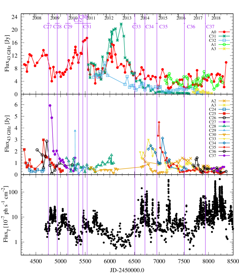
We have also modelled Stokes $Q$ and $U$ visibility data for components detected in the total intensity images, following the technique described in Jorstad et al. (2007). For comparison with multi-wavelength light curves and polarization curves analysed in this paper, we have calculated at each epoch total and linearly polarized flux densities and electric vector position angles, EVPA, by summing the $I_{i}$, $Q_{i}$ and $U_{i}$ flux densities from all components $i$ of the source at each epoch. We have constructed a total flux density light curve at 43 GHz, $F_{\rm total}$, representing the sum of the flux densities of all components, and curves of the degree of polarization in percentage, $P=\sqrt{(F_{Q,{\rm total}}^{2}+F_{U,{\rm total}}^{2})}/F_{\rm total}\times 100$ percent, and EVPA in degrees, EVPA=$0.5{\rm arctan}(U_{\rm total}/Q_{\rm total})$. The light curve at 43 GHz is presented in Figure 2, and the polarization parameters at 43 GHz versus epoch are given in Fig. 15.

2.6 Optical polarimetry

In this study, we include optical polarimetric data obtained with telescopes at the Crimean Astrophysical Observatory, St. Petersburg University, Lowell Observatory (Perkins Telescope), Steward Observatory, and Calar Alto Observatory. The Galactic latitude of 3C 279 is 57°and $A_{V}$ = 0.078 mag, so that interstellar polarization (ISP) in its direction is $<0.3$ per cent. To correct for ISP, the mean relative Stokes parameters of nearby stars were subtracted from the relative Stokes parameters of the object. This removes the instrumental polarization as well, under the assumption that the stellar radiation is intrinsically unpolarized. The fractional polarization has been corrected for statistical bias, according to Wardle & Kronberg (1974). For some of our analysis (see §3.7), we resolve the $\pm 180\degr$ ambiguity of the polarization electric-vector position angle (EVPA) by adding/subtracting $180\degr$ each time that the subsequent value of the EVPA is $>90\degr$ less/more than the preceding one.

2.7 Spectroscopic observations

We performed spectral observations of 3C 279 with the 4.3 m Discovery Channel Telescope (DCT, Lowell Observatory, telescope located in Happy Jack, AZ, USA) using the DeVeny spectrograph and Large Monolithic Imager (LMI). The DeVeny spectrograph, with 300 grooves per mm and a grating tilt of 22$\aas@@fstack{\circ}$35, was employed to produce a spectrum from 3500Å  to 7000Å, centred at 5000Å, with a dispersion of 2.2 Å/pixel and a pixel size of 0.253 arsec. We used a slit width of 2.5 arcsec. The technique for the spectral observations and data reduction was adapted from that developed at the NASA Infrared Telescope Facility for observations with SpecX (Vacca et al., 2003), which is based on an observation of a ‘telluric standard’ whose intrinsic spectrum is known. This allowed derivation of a system throughput curve, which was then applied to the spectrum of the source. Each spectral observation of 3C 279 included 2-3 exposures of 900 s each. A calibration star, HD 112587, of spectral type A0 and located $<1\degr$ from 3C 279, was observed just before and after the quasar, with two exposures of 60 s each. The exposure lengths of the target and telluric standard varied slightly, depending on the brightness of 3C 279 and weather conditions. Since the DCT is capable of switching between different instruments within 2-3 minutes, the spectral observations were followed by photometric observations of the quasar in $R$ and $V$ bands with the LMI in order to determine the flux calibration. Bias and flat-field images were obtained for corresponding corrections for both instruments.

3 RESULTS AND DISCUSSION

3.1 Flux and colour evolution

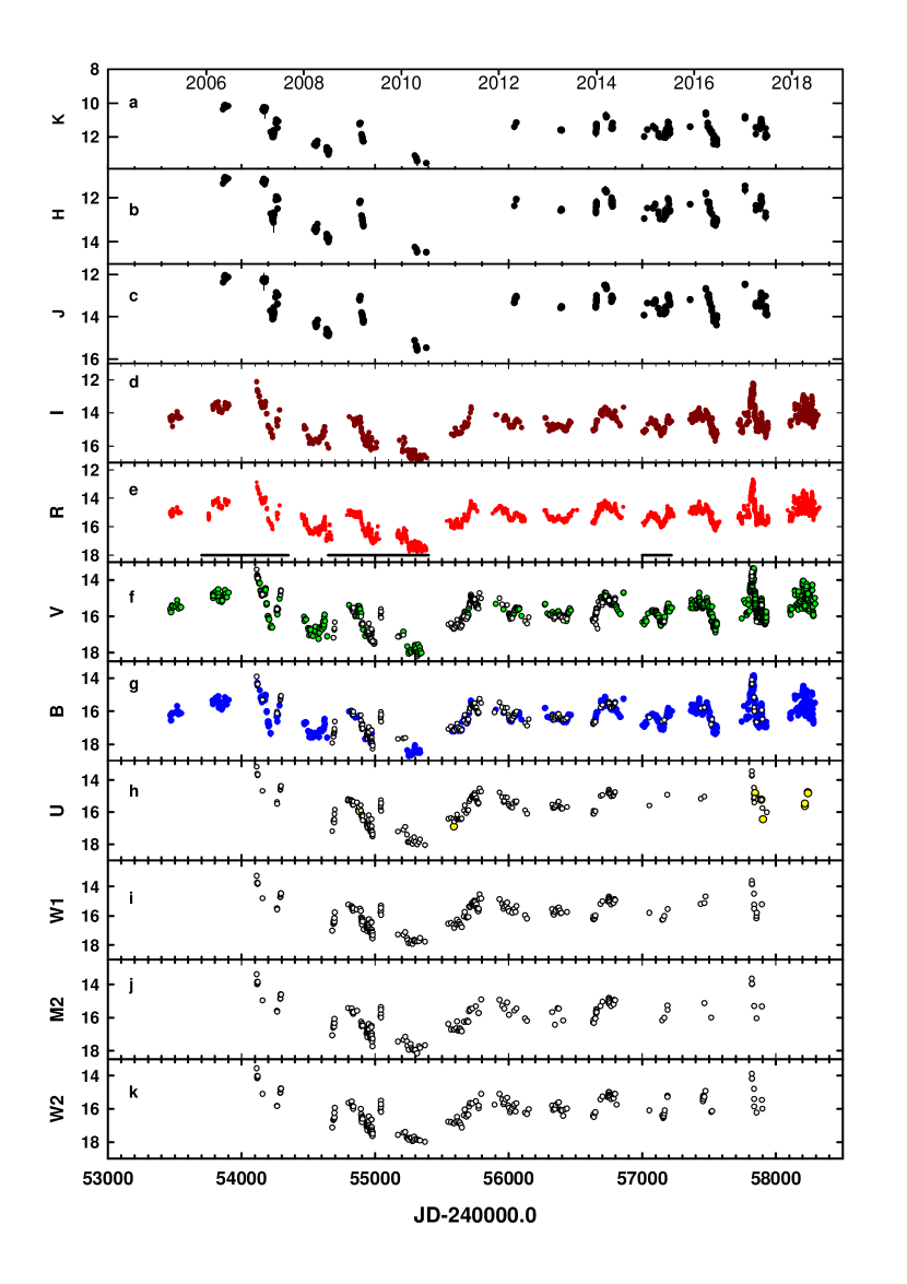
The optical light curves of 3C 279, collected by the WEBT participating teams during the 2007–2018 time interval, are shown in Fig. 1 (a-k); horizontal lines in panel (e) mark the data published in earlier WEBT-GASP papers (Böttcher et al., 2007; Larionov et al., 2008; Hayashida et al., 2012; Pittori et al., 2018). In panels (f-k) of the same figure we show Swift UVOT data (open circles). As is common for the WEBT campaigns, the data coverage in the optical range is dense (nearly 5000 data points in $R$ band, 1000–1500 in $B$, $V$ and $I$) throughout each observational season. The most intensive observations were performed during high-activity states of the blazar.

Figure 1: Optical, near-infrared, and ultraviolet light curves of 3C 279 over the time interval of the WEBT campaign. Horizontal lines in panel (e) mark the data published in earlier WEBT-GASP papers (Böttcher et al., 2007; Larionov et al., 2008; Hayashida et al., 2012; Pittori et al., 2018). Empty circles in panels (f) through (k) refer to the Swift data

.

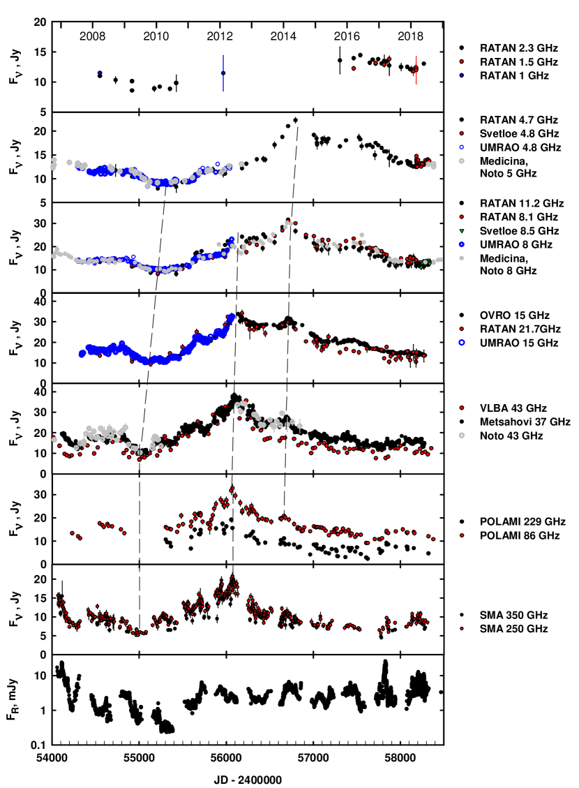
Radio flux densities versus time are plotted in Fig. 2. The 43 GHz light curve is constructed based on the VLBA images as described in §3.5. Slanted dashed lines connect minima and maxima in the different light curves, which may correspond to the same emission events of 3C 279 at different frequencies.

Figure 2: Radio light curves of 3C 279 over the time interval 2007–2018. For comparison, the $R$ band light curve is reproduced in the bottom panel. Dashed slanted lines connect positions of main extrema of the light curves (see § 3.4.3).

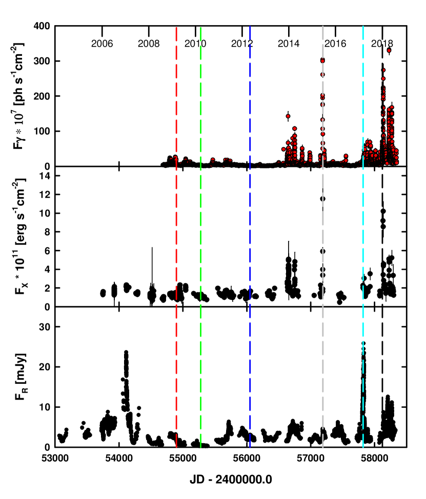
We plot the high-energy (Fermi LAT and Swift XRT) light curves in Fig. 3. Visual inspection reveals that the general patterns of the $\gamma$-ray and X-ray light curves are quite similar.

Figure 3: High-energy light curves of 3C 279 over the time interval 2006–2018. For comparison, the $R$ band light curve is reproduced in the bottom panel. Dashed vertical lines mark epochs when SEDs were constructed (see § 3.3).

The question of whether a blazar’s optical radiation becomes redder or bluer when it brightens is a topic of numerous papers. It is commonly agreed that the relative contributions of the big blue bump (BBB) and Doppler-boosted synchrotron radiation from the jet differ between quiescence and outbursts, and that this is one factor that leads to variability of the SED. In a recent paper, Isler et al. (2017) have parametrized optical-NIR variablity of 3C 279 in terms of the combined contributions of the accretion disc and the jet. However, most previous studies are qualitative rather than quantitative, owing to the difficulty in evaluating the contributions of constant and slowly-varying components, such as starlight from the host galaxy, the accretion disc, and the broad emission-line region.

A straightforward way to isolate the contribution of the component of radiation that is variable on the shortest time scales (presumably, synchrotron radiation) has been suggested by Hagen-Thorn (see, e.g., Hagen-Thorn et al., 2008, and references therein). The method is based on plots of (quasi)simultaneous flux densities in different colour bands and the construction of the relative continuum spectrum based on the slopes of the sets of flux-flux relations thus obtained. This method was successfully applied for the quantitative analysis of the synchrotron radiation of several blazars, for example, 0235+164 (Hagen-Thorn et al., 2008); 3C 279, BL Lac, and CTA 102 (Larionov et al., 2008; Larionov et al., 2010; Larionov et al., 2016b); 3C 454.3 (Jorstad et al., 2010); and 3C 66a, S4 0954+65, and BL Lac (Gaur et al., 2019).

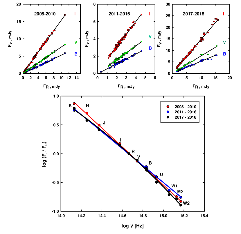
We adopt the same approach, as displayed in Fig. 4, where the flux densities of 3C 279 in $B$, $V$ and $I$ bands are plotted against the $R$-band flux density. The three plots in the top panels, obtained during different intervals of enhanced activity, together with analogous dependencies in UV and NIR bands, allow a derivation of the relative spectrum of the variable component, plotted in the bottom panel of the same figure. With this, we are able to trace the seasonal changes of the spectral index $\alpha$ (in the sense $F_{\nu}\propto\nu^{-\alpha}$) over the entire UV–NIR range. We split the time range into three parts, determined via visual inspection of Fig. 1: 2008–2010 (period of general decline of the flux, down to the unprecedented low level of 2010), 2011–2016 (modest level of activity over the optical range), and 2017-2018 (enhanced mean flux and short time-scale variations in the optical bands). We obtain $\alpha=1.65\pm 0.02$ for 2008–2010, $\alpha=1.47\pm 0.02$ for 2011–2016, and $\alpha=1.60\pm 0.02$ for 2017–2018. The values of the slopes refer to the central frequency, corresponding to $R$ band. We emphasize that these values are for the variable component only, not for the total flux density. We also find mild curvature (convexity) of the spectrum of the variable (synchrotron) component over the interval 2017–2018, i.e., a softening of the spectrum, despite elevated flux levels across the entire UV-optical frequency range (see Figures 1, 3). We note that a very similar value of $\alpha=1.58\pm 0.01$ in 2006–2007 was reported by Larionov et al. (2008).

Figure 4: Flux-flux dependencies of $F_{B}$, $F_{V}$ and $F_{I}$ vs $F_{R}$ (upper row of panels). Relative continuum spectrum of variable component of radiation from UV through NIR bands (bottom panel).

3.2 Optical spectra and variability of broad emission-line clouds

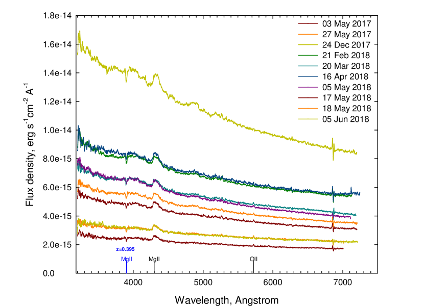
We analyse the optical spectroscopic behaviour of 3C 279 using data obtained at the 4.3 m Discovery Channel Telescope (DCT). Figure 5 displays our spectra of 3C 279 from the 2017 and 2018 observing seasons. All of these spectra contain a prominent Mg ii $\lambda 2800$Å  broad emission line redshifted to $\lambda 4280$Å. In addition to this prominent feature, we also mark in the figure the low-redshift absorption line of Mg ii at $\lambda 3906$Å  arising in a foreground galaxy at $z=0.395$ (see Stocke et al., 1998). We also mark an emission line of O ii, intrinsic to 3C 279. We note that there are a number of broad spectral features between $\lambda 3600$ and 5300Å (rest wavelengths in the 2350-3450Å range), often called the ‘little blue bump’ and attributed to many blended Fe lines (e.g., Vestergaard & Wilkes, 2001).

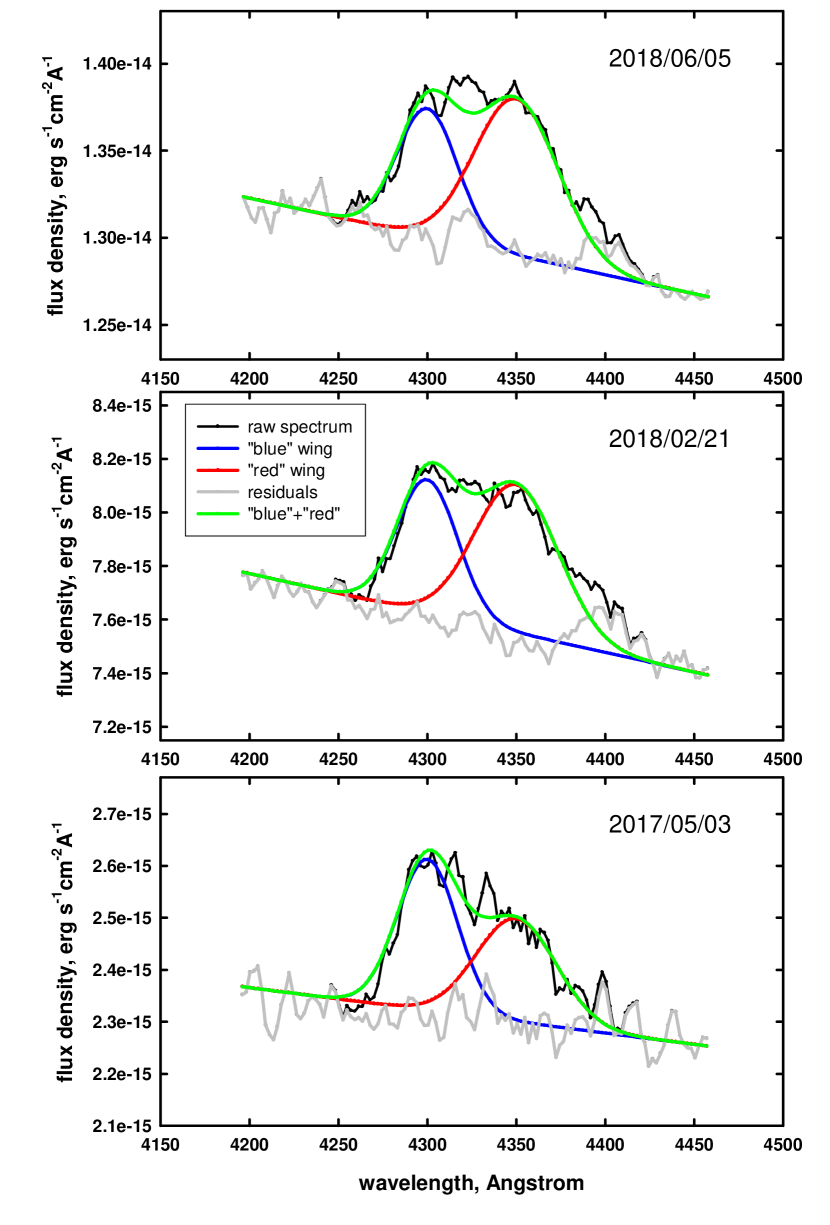
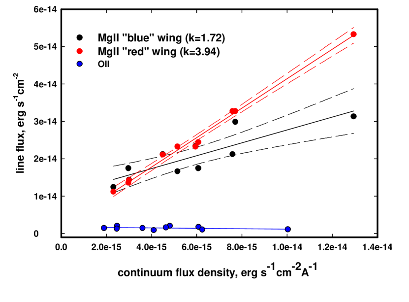
Visual inspection of the spectra displayed in Figure 5 reveals that (1) the line flux of Mg ii correlates with the continuum flux and (2) there is marked asymmetry (‘red wing’) to this line, as previously noted by Punsly (2013). We deblend the observed line profiles, fitting them with two Gaussian functions superposed on a featureless continuum. Examples of the fit are given in Figure 6. The wide range of continuum flux densities, seen in Figure 5, allows us to plot the dependencies of the fluxes in the ‘blue’ and ‘red’ components of Mg ii on the continuum flux; see Figure 7. This definitive correlation is similar to that found in the Mg ii line of quasar 3C 454.3 by León-Tavares et al. (2013). Less pronounced line flux variability in the spectra of several blazars has also been reported by Isler et al. (2015). In contrast, stability of emission-line fluxes has been reported in several previous studies: 3C 454.3 (Raiteri et al., 2008), PKS 1222+216 (Smith et al., 2011), 4C 38.41 (Raiteri et al., 2012), OJ 248 (Carnerero et al., 2015), and CTA 102 (Larionov et al., 2016b).

Figure 5: Spectra of 3C 279 during the 2017 and 2018 observing seasons.

Figure 6: Examples of Gaussian fitting of the Mg ii line profile for different levels of the continuum flux.

Figure 7: Dependencies of Mg ii line fluxes vs. continuum flux density. The 95% confidence intervals are also shown. For comparison, the dependence of [O  ii] $\lambda_{\mathrm{rest}}$ 3727Å  flux vs. the adjacent continuum flux density is plotted near the bottom.

The two-component profile of the Mg ii line in 3C 279 could be explained by radial infall of matter onto the accretion disc surrounding the central black hole. The speed of the ‘red’ component is then $\sim$3500 km s^-1, corresponding to a $\sim$50 Å  wavelength shift of that component. The free-fall velocity of matter at a distance $R_{\rm pc}$ pc from a black hole of mass $M_{9}=10^{9}$ M☉  is $v_{\rm in}=2940(M_{9}/R_{\rm pc}^{1/2})$ km s^-1. As reported in Nilsson et al. (2009), the most reliable estimate of the black hole mass in 3C 279 is $10^{8.9}$ M☉, hence the free-fall velocity is $\sim 3500$ km s^-1 at $R_{\rm pc}\sim 0.6$ pc.

Another approach (Corbin, 1997) suggests that the redward profile asymmetries can be produced by the effect of gravitational redshift on the emission from a ‘very broad line region,’ provided that this region takes the form of a flattened ensemble of clouds viewed nearly face-on and with a mean distance of a few tens of gravitational radii from the black hole. The effect of gravitational redshift of the line emitted from a source at a distance $R_{\mathrm{source}}$ from the black hole is given by

$$\frac{\lambda_{\mathrm{obs}}}{\lambda_{\mathrm{source}}}=(1-\frac{R_{\mathrm{Sch}}}{R_{\mathrm{source}}})^{-1/2}$$ (1)

Here $R_{\mathrm{Sch}}=2GM/c^{2}$ is the Schwarzschild radius of the central black hole with mass $M$. The displacement of the red component of Mg ii of $\sim$50Å  (see Fig. 6) corresponds to a position of the emitting cloud of $\sim$43$R_{\mathrm{Sch}}\approx 3\times 10^{-3}$pc, or about 4 light-days, from the black hole. While this is closer than expected to the black hole for a cloud emitting Mg ii lines, which do not require high ionization parameters, we note that such small distances of emission-line regions from black holes have been inferred from microlensing studies of quasars (Guerras et al., 2013).

We measure the Mg ii line FWHM for both the ‘blue’ and ‘red’ components, from which one can derive the velocity dispersion of the gas clouds in the broad-line region (BLR) and obtain, correspondingly, $v_{\mathrm{blue}}=3450\pm 200\>\mathrm{km\>s^{-1}}$ and $v_{\mathrm{red}}=3800\pm 200\>\mathrm{km\>s^{-1}}$ . These values are lower limits to the actual velocity range of the clouds, since the expected velocity dispersion depends on the geometry and orientation of the BLR (see, e.g., Wills & Brotherton, 1995). In fact, because the line of sight to a blazar is probably nearly perpendicular to the accretion disc, the de-projected velocity range is likely to be a factor $\gtrsim 2$ higher than the FWHM given above if the BLR is in the disc.

The strong relationship between the optical (and presumably UV) continuum and the emission-line flux suggests that the radiation responsible for the excitation of the broad Mg ii lines comes mostly from the jet. This is difficult to reconcile with the gravitational redshift hypothesis for the displacement of the red wing, since the optical emission from the jet is unlikely to be highly beamed only several light-days from the black hole (see Marscher et al., 2010). If the dominant exciting radiation instead were to arise in the accretion disc, we would not expect to see such a strong correlation between the synchrotron continuum and line flux: the only direct association of flare and superluminal knot production in the jet with an event in the accretion disc corresponds to a decrease in the optical-ultraviolet flux of the disc (in the radio galaxy 3C 120; Marscher et al. 2018). Since the jet emission is expected to be highly beamed by a Doppler factor $\sim 20$ (Jorstad et al., 2017), the association of variations in emission-line flux with beamed synchrotron radiation from the jet implies that the clouds responsible for these lines lie within $\sim 10\degr$ of the jet axis, as proposed by León-Tavares et al. (2015).

The deblending of the Mg ii line discussed above does not take into account possible contribution of time-variable Fe ii emission lines. Fe ii lines are present over a wide range of wavelengths near the Mg ii line and should be present under the physical conditions that produce strong Mg ii emission. We note that Patiño-Álvarez et al. (2018) conclude that Fe ii emission is negligible in the vicinity of the Mg ii line in the spectra of 3C 279 that they have studied. Nevertheless, given the presence of a strongly time-variable red wing to the Mg ii line, which is difficult to explain physically (see above and Punsly, 2013), we plan to carry out a more thorough analysis of Mg and Fe line emission in a future study.

Based on the above considerations, we tentatively conclude that the variable, displaced (by 3500 km s^-1) component of the Mg ii emission line arises from infalling clouds located $\sim 0.6$ pc from the black hole and outside the jet, but within $\sim 10\degr$ of the jet axis.

3.3 Spectral energy distributions

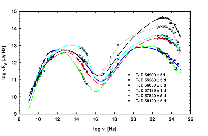
Figure 8 presents the SED (${\rm log}\,\nu F_{\nu}$ vs. log $\nu$) of 3C 279 at 6 epochs with different levels of activity, displaying the usual double-hump shape. We follow the common interpretation that the humps correspond to synchrotron radiation at lower frequencies and inverse Compton (IC) scattering at high energies. The epochs, which are also marked in Figure 3, include TJD 58120 when the $\gamma$-ray to optical-IR flux ratio at the corresponding peaks was $\sim 60$, as well as other epochs when it was closer to unity. As has been discussed by Sikora et al. (2009), the flux ratio should not greatly exceed unity if the $\gamma$-ray emission occurs via the synchrotron self-Compton (SSC) mechanism corresponding to IC scattering of synchrotron photons from the jet, with the same population of electrons responsible for both processes. Otherwise, the seed photons for the scattering are likely generated from outside the jet (external Compton, or EC, radiation). Among the six SEDs displayed in Figure 8, only two epochs (TJD 57189 and 58120) are inconsistent with SSC $\gamma$-ray emission solely on this basis. One of these (TJD 57820) includes the highest optical flux found in our study; the flux of the peak of the $\gamma$-ray SED was only a factor of $\lesssim 4$ higher than that of the synchrotron peak.

The SED should generally rise with frequency up to a point $\nu_{\rm peak}$ where the spectral index steepens to unity. This corresponds to the critical frequency of electrons with energy per unit rest mass $\gamma_{\rm peak}$, at which the energy distribution steepens to $N(\gamma)\propto\gamma^{-3}$. In some models, this occurs at a break in the injected electron energy distribution (e.g., Sikora et al., 2009), while in others there is a more gradual downturn of a log-parabolic energy distribution (e.g., Massaro et al., 2006). In the model of Marscher (2014), the volume filling factor of the highest-energy electrons is inversely proportional to energy owing to variations in magnetic field direction relative to shock fronts. This causes a steepening of the energy distribution when averaged over the entire volume. The shock model of Marscher & Gear (1985) produces a break from radiative energy losses at an energy that evolves with time as the shock moves down the jet.

If we tentatively assume that the $\gamma$-ray portion of the SED on TJD 57820 is produced by SSC emission, we can estimate the value of $\gamma_{\rm peak}$ as

$$\gamma_{\rm peak}\sim[\nu^{\rm SSC}_{\rm peak}/\nu^{\rm S}_{\rm peak}]^{1/2}\sim 4\times 10^{4},$$ (2)

where we have taken $\nu^{\rm SSC}_{\rm peak}\sim 5\times 10^{13}$ Hz (see Fig. 8). The corresponding magnetic field strength is

$$B\sim[\nu^{\rm S}_{\rm peak}(1+z)]/[(2.8\times 10^{6}~{}{\rm Hz})\gamma_{\rm peak}^{2}\delta]~{}{\rm G}\sim 4\times 10^{-4}~{}{\rm G}$$ (3)

(e.g., Rybicki & Lightman, 1979), where $\delta$ ($\sim 40$ in 2017; see §3.5 below) is the Doppler beaming factor and $z=0.538$ is the redshift of 3C 279. This is implausibly low for a compact emission region on parsec scales; hence we conclude that even for the flare on TJD 57820 with such a high synchrotron amplitude, the $\gamma$-ray emission was produced by the EC process. SSC emission could have dominated on TJD 54900 and 55280 when the $\gamma$-ray to synchrotron flux ratio was $\lesssim 1$ and the value of $\nu^{\gamma}_{\rm peak}$ was relatively low, but the absence of flux measurements at the SED peaks at these epochs precludes an accurate assessment of this possibility.

In the case of EC emission, which we infer to apply to the outbursts of 3C 279 with the highest fluxes (as concluded earlier by Sikora et al., 2009; Hayashida et al., 2015; Ackermann et al., 2016), the frequency of the peak in the $\gamma$-ray SED is given by

$$\nu^{\rm EC}_{\rm peak}\approx\nu^{\prime}_{\rm seed}\gamma_{\rm peak}^{2}\delta(1+z)^{-1}\propto\nu_{\rm seed}\Gamma\delta(1+z)^{-1},$$ (4)

where $\nu_{\rm seed}\approx\nu^{\prime}_{\rm seed}\Gamma^{-1}$ is the frequency of the peak in the SED of the seed photons in the host galaxy rest frame, and $\Gamma$ is the bulk Lorentz factor of the emitting plasma. Note that $\nu^{\rm EC}_{\rm peak}$ is approximately proportional to $\delta^{2}$ if $\Gamma\sim\delta$, as is expected to be the case for blazars. An increase in the Doppler factor should increase both the flux and frequency of the SED peak. While an increase in the latter is not evident in the SEDs displayed in Figure 8, the SEDs of very sharp flares on time scales of minutes to hours in 3C 279 have exhibited an increase in $\nu^{\rm EC}_{\rm peak}$ (Hayashida et al., 2015; Ackermann et al., 2016) during maximum flux.

In general, a rise in flux involves some combination of an increase in the number of radiating particles, the magnetic field strength, the Doppler beaming factor, and the energy density of seed photons, $u_{\rm seed}$. Radiative energy losses of the highest-energy electrons tend to be severe during outbursts in 3C 279 (Sikora et al., 2009; Hayashida et al., 2015; Ackermann et al., 2016), so that essentially all of the energy that the electrons obtain from particle acceleration is transferred to electromagnetic radiation. Increases in apparent luminosity require an increase in either the number of these electrons or the Doppler beaming factor.

Figure 8: Quasi-simultaneous spectral energy distributions of 3C 279. TJD is truncated Julian date, JD$-$2400000

Although the peak frequency of the synchrotron SED is determined only within about an order of magnitude, this is sufficient to specify that the ratio of the IC to synchrotron peak frequencies is $10^{9\pm 0.5}$. The Lorentz factor (energy in rest-mass units) of the electrons radiating at the EC and synchrotron SED peaks should be the same and given by

$$\gamma_{\rm peak}\sim[\nu^{\rm EC}_{\rm peak}(1+z)/(\delta\nu^{\prime}_{\rm seed})]^{1/2},$$ (5)

where $\nu^{\prime}_{\rm seed}$ is the frequency of the maximum of the seed photon SED as measured in the frame of the radiating plasma. Equation 3 then allows us to derive the magnetic field strength. Based on the TJD 57189 SED, when the peak IC flux was $\sim 40$ times the peak synchrotron flux, indicating dominance by the EC process, we express the parameters as $\nu^{\rm S}_{\rm peak}=10^{14}\nu^{S}_{\rm peak,14}$ Hz, $\nu^{\rm EC}_{\rm peak}=10^{23}\nu^{C}_{\rm peak,23}$ Hz, $\nu^{\prime}_{\rm seed}=10^{16}\nu^{\prime}_{\rm seed,16}$ Hz, and, from apparent superluminal motions, $\delta=20\delta_{20}$ and $\Gamma=20\Gamma_{20}$ (Jorstad et al., 2017). Equation 5 then becomes

$$\gamma_{\rm peak}\sim 900[\nu^{\gamma}_{\rm peak,23}(1+z)/(\delta_{20}\nu^{\prime}_{\rm seed,16})]^{1/2}.$$ (6)

If the seed photons are primarily from the little blue bump (the Ly$\alpha$ emission line is not very strong in 3C 279; Stocke et al., 1998), so that $\nu_{\rm seed}\sim 10^{15}$ Hz, $\nu^{\prime}_{\rm seed,16}\sim 2\Gamma_{20}$, $\gamma_{\rm peak}\sim 800$, and $B\sim 4$ G. Even with such a low value of $\gamma_{\rm peak}$, the radiative cooling time of the electrons in the plasma frame is only $7.8\times 10^{8}[B^{2}+[(u^{\prime}_{\rm seed})^{2}/(8\pi)](\gamma^{\prime}_{\rm peak})^{-1}\sim 40$ s (dominated by EC losses that are $\sim 40$ times stronger than synchrotron losses given the flux ratios of the two SED humps), allowing for rapid variability (although limited by the light-crossing time across the region). If, on the other hand, the seed photons correspond to blackbody radiation from dust with a temperature $\sim 1200$ K (as in 4C21.35; Malmrose et al., 2011), $\nu^{\prime}_{\rm seed,16}\sim 0.05\Gamma_{20}$, $\gamma_{\rm peak}\sim 5000$, and $B\sim 0.1$ G. In this case, the radiative cooling time is $\sim 10^{4}$ s in the plasma frame and $\sim 10^{3}$ s in the observer’s frame. Intra-day flux variations are therefore possible in either case if the size of the emission region is $\lesssim 0.01\delta_{\rm 20}$ pc.

Another possible source of seed photons is synchrotron radiation from a relatively slow (and, correspondingly, less beamed) Mach disc (Marscher, 2014) or sheath of the jet (MacDonald et al., 2015). As suggested by Marscher et al. (2010), such slowly moving plasma could produce the requisite number of seed photons while being too poorly beamed to contribute substantially to the observed optical flux. Stacked multi-epoch VLBA images have confirmed the existence of sheaths in the jets of several blazars, including 3C 279 (MacDonald et al., 2017). The peak of the SED of such synchrotron photons is likely to be in the far-IR range, in which case the above estimate of the magnetic field for seed photons from hot dust should be applicable.

A major difference between EC from polar emission-line clouds or slowly moving jet plasma and EC from dust is the possibility of variations in the former case, while dust is expected to provide a steady source of seed photons. Variability of the seed photons can explain the general absence of repeated episodes of variability with nearly identical patterns of temporal behaviour.

3.4 Inter-band correlations

3.4.1 $\gamma$-ray – X-ray correlations

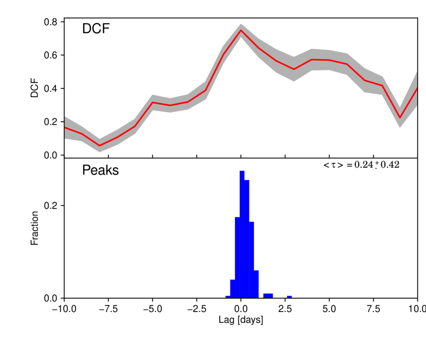
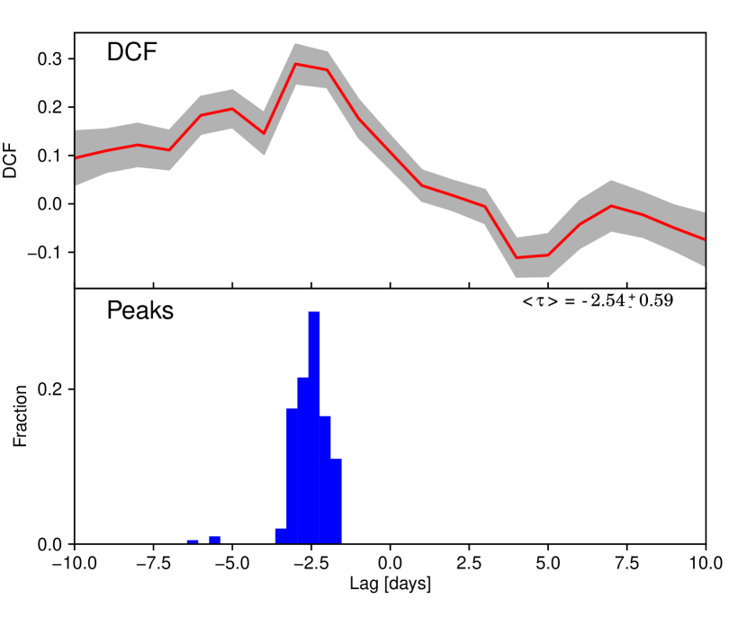
We calculate the discrete correlation function (DCF) (Edelson & Krolik, 1988; Hufnagel & Bregman, 1992) between the $\gamma$-ray and X-ray flux variations of 3C 279 during 2008–2018. We determine the significance of the correlation via the flux redistribution – random sub-sample selection method (see, e.g. Peterson et al., 1998). The results are presented in Figure 9, which reveals a strong correlation with a peak DCF of $0.75\pm 0.03$ and a delay of the $\gamma$-ray behind X-ray variations of 0.24$\pm$ 0.42 days, statistically consistent with zero lag. This implies that the correlation is significant at a level higher than p=0.001 per cent (e.g., Bowker & Lieberman, 1972) and conforms with Figure 3, which shows that every X-ray flare has a $\gamma$-ray counterpart and vice versa.

Figure 9: Upper panel: DCF between $\gamma$-ray and X-ray light curves of 3C 279 in 2008–2018. Positive delays correspond to X-ray leading $\gamma$-ray variations. Bottom panel: Distribution of lags of maxima of the DCF from 200 Monte Carlo simulations with flux redistribution and 67% bootstrapping. The grey area in the upper panel correspond to $\pm 1\sigma$ spread of simulated DCFs.

3.4.2 $\gamma$-ray – optical correlations

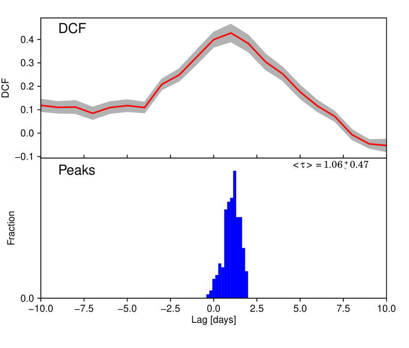
In a similar way, we calculate the DCF between the optical and $\gamma$-ray flux variations. The resulting correlation, given in Fig. 10, is rather weak, with a maximum DCF of 0.42. There is a delay on the level of $2\sigma$ between the variations in the two energy bands, with the $\gamma$-ray leading the optical variability by $1.06\pm 0.47$ days. The optical and $\gamma$-ray light curves of 3C 279 are quite complex, with ‘sterile’ (optical without $\gamma$-ray counterpart) and ‘orphan’ ($\gamma$-ray without optical counterpart) flares occurring in both energy ranges. To estimate the statistical significance of the correlation between $\gamma$-ray and optical variations, we have performed a Monte-Carlo simulation in the following way. At first, we approximated both $\gamma$-ray and optical light curves with a set of double-exponential functions in a manner similar to Abdo et al. (2010). After obtaining the statistical distributions of peak parameters $(f_{\mathrm{max}},t_{\mathrm{raise}},t_{\mathrm{decay}})$, we generated a set of synthetic light curves by co-adding random peaks drawn from these distributions and placed into random positions. Any correlation between these synthetic light curves is by random chance, so by computing the correlation between them we can estimate the probability of a spurious correlation at a given level. Among $10^{4}$ artificial light curves generated in this manner, none gave a correlation coefficient equal to or higher than the observed value of 0.4. Therefore, we can consider this correlation level as statistically significant at the 0.01 per cent level.

Figure 10: Upper panel: DCF between optical and $\gamma$-ray light curves of 3C 279 in 2008–2018. Positive delays correspond to $\gamma$-ray leading optical variations. Bottom panel: Distribution of lags of maxima of the DCF after 200 Monte Carlo simulations with flux redistribution and 67% bootstrapping. The grey area in the upper panel correspond to $\pm 1\sigma$ spread of simulated DCFs.

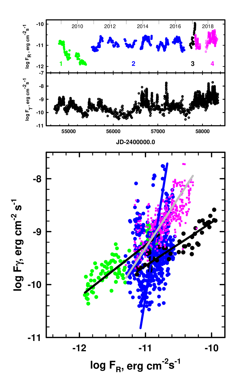
This short delay between $R$-band and $\gamma$-ray variations allows us to compare directly the optical and $\gamma$-ray light curves. To do this, we bin the $R$-band optical data so that the mid-point and size (in time) of each optical bin corresponds to those of the respective $\gamma$-ray bin. Figure 11, where we plot the optical (upper panel) and $\gamma$-ray (middle panel) light curves, and $\gamma$-ray flux versus $R$ band flux (bottom panel), demonstrates clear differences in the optical/$\gamma$-ray relationship during the various stages of activity of 3C 279. The slopes of $\log F_{\gamma}-\log F_{R}$ dependencies, for time intervals (1) through (4) (as marked in the upper panel of that figure), are correspondingly: (1) $0.97\pm 0.04$, (2) $7.7\pm 1.2$, (3) $0.82\pm 0.06$ and (4) $1.90\pm 0.09$. The slope of the dependence therefore changes dramatically, starting from $\sim 1$ (2008–2010), then switching to $\sim 8$ (2011–2016). The onset of optical and $\gamma$-ray activity that occurred in late 2016 altered the slope again to $\sim 1$. Shortly after the maximum of the optical outburst, the slope changed again, to $\sim 2$. Remarkably, unlike transitions from the slope of 1 to 8 and back to 1, where the changes seem to have happened during seasonal gaps, the last change appears to have occurred over a few days, TJD 57837$\pm 2$. It is tempting to find some event(s) that accompanied this switch from linear to quadratic slope. The only change in other observed parameters that is simultaneous with this transition is a short-term drop of the optical polarization degree to 1.5% during the night of optical maximum. However, as can be seen from Fig. 15, there are several other incidents of low polarization, with no obvious physical reason to connect these two events.

The $\gamma$-ray flux in Figure 11 is derived by multiplying the photon flux (see § 2.3) by an integral over a fixed log-parabolic energy distribution. It is therefore directly proportional to the photon flux, which in turn is proportional to the flux density divided by frequency. The synchrotron flux is the flux density times the fixed observed R-band frequency (which is above the frequency of the peak in the synchrotron SED). From relativistic beaming alone, we then expect the dependencies on Doppler factor to be $F_{\gamma}\propto\delta^{2+\alpha_{\gamma}}$ and $F_{\rm opt}\propto\delta^{3+\alpha_{\rm opt}}$ (see Dermer, 1995). Since the peak of the $\gamma$-ray SED is usually in the LAT range except during low states (cf. Fig. 8), we adopt $\alpha_{\gamma}=1.0$ for the $\gamma$-ray spectral index, while in §3.1 we derived the spectral index of the variable optical component to be $\alpha_{\rm opt}=1.56\pm 0.11$.

As found by Sikora et al. (2009), Hayashida et al. (2015), and Ackermann et al. (2016), the $\gamma$-ray and optical emission is so luminous that the electrons lose nearly all of their energy to EC radiation on time scales shorter than the light-travel time across the emitting region. In this fast-cooling case, the ratio of $\gamma$-ray to optical flux (as defined above) is proportional to the ratio of EC radiative losses to synchrotron losses, which in turn is proportional to $u^{\prime}_{\rm seed}/B^{2}\propto u_{\rm seed}\Gamma^{2}/B^{2}$. An increase in the number of radiating electrons $N_{\rm re}$ increases proportionately the luminosity of the dominant emission process, which is EC $\gamma$-ray production during the higher-flux states in 3C 279. The ratio of EC to synchrotron luminosity is affected by changes in the magnetic field $B$ or energy density of seed photons (as measured in the emitting plasma frame), which can occur if (i) the plasma moves toward or away from the source of the seed photons, (ii) more seed photons are produced near the jet, or (iii) the bulk Lorentz factor $\Gamma$ changes (since the energy density of the seed photons in the plasma frame $u^{\prime}_{\rm seed}\propto\Gamma^{2}$).

We can consider a number of cases of different physical parameters changing, each with its own dependence between $\gamma$-ray and optical flux. We parametrize the optical/$\gamma$-ray flux relationship as $F_{\gamma}\propto F_{\rm opt}^{\zeta}$. Based on arguments given in §3.3, here we assume that the EC process dominates the $\gamma$-ray production.

1. An increase solely in the number of radiating electrons $N_{\rm re}$ should cause the synchrotron and EC flux to rise by the same factor, so that $\zeta\approx 1$. The frequencies of the SED peaks should remain the same unless there is a change in the energy at which the slope of the electron energy distribution becomes steeper than $-3$.

2. An outburst can result from a higher Doppler factor owing to bending toward the line of sight of the emitting region. This can occur if the entire jet changes its direction (wobbles or precesses), or if different parts of the jet cross-section with various velocity vectors relative to the mean become periodically or sporadically bright as time passes. A possible realisation of such behaviour in the case of CTA 102 was suggested by Larionov et al. (2017). The flux during such events should follow the beaming-only relationships given above, with $F_{\gamma}\propto\delta^{3}$ and $F_{\rm opt}\propto\delta^{4.56}$, hence $\zeta\approx 0.7$. The frequency of the SED peaks of both the synchrotron and EC emission should obey $\nu_{\rm peak}\propto\delta\propto F_{\gamma}^{1/3}$.

3. An increase in bulk Lorentz factor $\Gamma$, and therefore Doppler factor, raises both the beaming and $u^{\prime}_{\rm seed}$, as well as $\nu_{\rm peak}$ of both the synchrotron and EC SEDs. The increase in the seed photon field actually decreases the synchrotron luminosity in the plasma frame, since EC scattering then consumes a higher fraction of the electron energies. If the plasma-frame EC luminosity is already dominant, then it will not increase much, since the electrons were already expending nearly all of their energy on EC emission. We then derive the rough dependence $F_{\rm opt}\propto\delta^{4.6}{u^{\prime}_{\rm seed}}^{-1}\propto\delta^{4.6}\Gamma^{-2}\propto\delta^{2.6}$ if we approximate that $\delta\propto\Gamma$. Since $F_{\gamma}\propto\delta^{3}$, we obtain $\zeta\approx 1.2$.

4. An increase solely in the magnetic field strength $B$ by a factor $f_{B}$ would cause the synchrotron flux to rise by a factor $f_{B}^{1+\alpha_{\rm opt}}$ while the frequency of the peak of the synchrotron SED increases by a factor of $f_{B}$. The EC flux would decrease slightly owing to the higher fraction of electron energy that goes into synchrotron radiation. In this case, $\zeta$ would be a small negative number.

5. An increase only in the energy density of seed photons $u_{\rm seed}$ by a factor $f_{\rm seed}$ – either because of changes within the source of the photons or because of a shift in position of the radiating plasma toward the source of seed photons – would cause the ratio of EC to synchrotron flux to rise in proportion to $f_{\rm seed}$, while the frequencies of the synchrotron and SSC peaks would remain constant. Without a change in the number of radiating electrons, the $\gamma$-ray flux would increase only slightly, but the synchrotron flux would decrease by a factor of $f_{\rm seed}^{-1}$. This would result in $\zeta\ll-1$, with the exact value changing with the level of dominance of the EC luminosity compared with the synchrotron power. If the number of electrons also increases to create a flare, then a high positive value of $\zeta$ is possible.

The value of $\zeta\approx 1$ during time interval (1) of Figure 11 agrees with scenario (i), but the higher frequency of the peak in the $\gamma$-ray SED (see Fig. 8) at higher flux levels suggests that cases (ii) or (iii) might apply despite their respectively lower (0.7) and higher (1.2) values of $\zeta$. The very high value of $\zeta$ and pronounced variations during interval (2) agree with the expectation of a combination of scenarios (i) and (v). This suggests that the sites of the high-amplitude flares during this period also involved steep gradients in the energy density of seed photons. In concert with our finding that emission-line fluxes in 3C 279 are proportional to optical (and presumably UV) continuum fluxes, with a time delay $<2$ months, this might be possible if the seed photons are stimulated by the synchrotron flares, providing more seed photons for inverse Compton scattering during subsequent flares.

During time interval (3) of Figure 11, which is limited to the highest-amplitude optical outburst, the value of $\zeta\approx 0.8$ is closest to that expected for scenario (iii), but this is contradicted by the relatively small $\gamma$-ray to optical flux ratio, $\lesssim 4$. The latter suggests either a rise in the magnetic field strength or a decrease in $u^{\prime}_{\rm seed}$. These considerations imply that an increase in both the magnetic field and number of radiating electrons, probably combined with a decrease in the seed photon field, occurred during interval (3), such that $\zeta$ adopted an intermediate value between cases (i), (iv), and (v).

The value $\zeta\approx 2$ during time interval (4) corresponds to a time of very high EC dominance (see Fig. 8). Perhaps a combination of scenarios (iii) and (iv) – changes in both bulk Lorentz factor and seed photon energy density – could give the observed value of $\zeta$.

Figure 11: From top to bottom: $R$ band log flux density light curve, with different colours and numerical marks corresponding to different stages of activity; logarithmic $\gamma$-ray flux light curve; optical – $\gamma$-ray flux-flux diagram. Slopes of the linear (on a logarithmic scale) fits are (1) $0.97\pm 0.04$, (2) $7.7\pm 1.2$, (3) $0.82\pm 0.06$ and (4) $1.90\pm 0.09$.

3.4.3 Radio-band correlations

Visual inspection of Figures 1 and 2 reveals that there are few common details in the optical and radio light curves that would allow one to test the possible existence of correlations and time lags between the two. If we compare the optical $R$-band and radio 250 GHz light curves, both of which have good sampling, we find only two intervals of common elevated flux level, TJD 54000–54300 and TJD 55800–56100, and a dip over TJD$\sim$55000–55300. However, close correspondence between different light curves as one considers lower radio frequencies, with time lags between them, are clearly visible. Before evaluating the time lags, we consider what the results of our analysis would be if we did not possess data at frequencies from 22 to 8 GHz. In this case, we would associate maxima observed at 350–37 GHz close to TJD 55100 with the maximum observed at 5 GHz on TJD$\sim$56800, deriving a delay between variations in these bands of $\sim 700$ days. This is certainly a mis-identification, as we readily see when including the 22–8 GHz data. The dashed slanted lines in Fig. 2 give a hint of the ‘real’ values of the delays, which are (across the widest span of frequencies) no more than 300 days.

The progressive smoothing with decreasing frequency and, eventually, the disappearance of the most prominent maximum at TJD 56100, are naturally explained by the increased volume of the jet at lower frequencies, which smooths out the fine structure of variability. However, this does not explain the appearance and progressive growth of the emission feature first seen at 100 GHz close to TJD 56600 and culminating at 5 GHz near TJD 56800. A possible explanation of these two, markedly different, kinds of behaviour, is the same as suggested in Raiteri et al. (2017): that of a twisted inhomogeneous jet. Within this approach, magnetohydrodynamic instabilities or rotation of the twisted jet cause different jet regions to change their orientation and hence their relative Doppler factors.

3.5 Jet kinematics

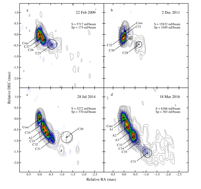
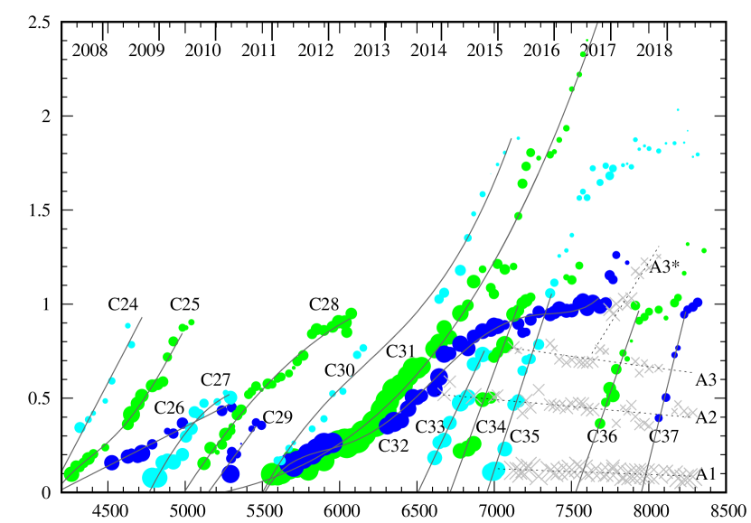
Figure 12 shows the total and polarized intensity VLBA images of 3C 279, convolved with an elliptical Gaussian beam that approximates the angular resolution at epochs when all 10 VLBA antennas operated. We follow the historical designation of moving components at 43 GHz started by Unwin et al. (1989); Wehrle et al. (2001), and continued by Jorstad et al. (2004); Jorstad et al. (2005); Chatterjee et al. (2008); Larionov et al. (2008), and Jorstad et al. (2017). During 2007-2018 we identify 14 moving knots in the jet, C24-C37 (see Fig. 13). Knots C24-C32 correspond to those identified by Jorstad et al. (2017). The apparent speed of the moving components, $\beta_{\rm app}$, has been determined using the same procedure as defined in Jorstad et al. (2005). Since almost all motions in 3C 279 are non-ballistic, in order to derive the most accurate values of the time of passage of a knot through the VLBI core, $T_{0}$, we use only those epochs when a component is within 1 mas of the core, inside of which its motion is assumed to be ballistic. Knots C30, C31, C32, C33, C34, and C35 can be associated with features C1, C2, C3, NC1, NC2, and NC3, respectively, in Rani et al. (2018). Table 3 shows angular, $\mu$ (in mas/yr), and apparent, $\beta_{\rm app}$ (in units of $c$), velocities, the ejection time, $T_{0}$, the average projected position angle with respect to the core, $\langle\Theta\rangle$, the average distance from the core when the knot is observed, $\langle R\rangle$, and the average flux density, $\langle F\rangle$, of knots ejected between 2007 and 2018 (partly adopted from Jorstad et al. (2017)). The derived apparent velocities are in the range from 5 to 37$c$. In addition to the core A0, we find three quasi-stationary components, A1, A2, and A3, located at $\sim$ 0.1, 0.5, 0.7 mas from the core, respectively. These knots appear in the jet after the ejections of very bright knots C31 and C32. Knots C30 - C37 exhibit especially rapid motions, with apparent velocities ranging from 20 to 37$c$. Components C36 and C37 decelerate significantly after reaching a distance of about 1 mas from the core. Knots C30 and C31 possess velocities up to $\sim 20c$ at distances $>$1.5 mas, factors of $\sim$ 2 and 3 times higher than those near the core, respectively. Table 4 lists times at which moving knots C35, C36, and C37 cross stationary components A1, A2 and A3, according their kinematics.

Figure 12: A set of VLBA images at 43 GHz in total (contours) and polarized (colour scale) intensity ($S$ and $Sp$, correspondingly) overlaid with fitted Gaussian circular components; the images are convolved with a beam of 0.36$\times$0.15 mas² at PA=-10$\degr$; linear segments within colour scale show direction of EVPA; four different epochs are chosen to show significant changes in the jet structure as discussed in § 3.5.

Figure 13: Separation of jet features from the core, A0, during 2007-2018, partly adopted from Jorstad et al. (2017). Each line or curve represents a polynomial fit to the motion of the respective knot. The diameter of each symbol is proportional to the logarithm of the flux density of the knot, as determined by model fitting of the VLBA data.

Table 3: Jet structure and kinematics

Knot	N	$\mu$(mas/yr)	$\beta_{\mathrm{app}}$	$T_{0}$(TJD)	$T_{0}$(year)	$\langle\Theta\rangle(\degr)$	$\langle R\rangle$(mas)	$\langle F\rangle$(Jy)
C24	7	$0.503\pm 0.031$	$16.01\pm 0.99$	$54064\pm 40$	$2006.90\pm 0.11$	$-125.4\pm 2.8$	$0.560\pm 0.210$	$0.43\pm 0.22$
C25	17	$0.386\pm 0.014$	$12.30\pm 0.43$	$54133\pm 33$	$2007.09\pm 0.09$	$-124.9\pm 13.1$	$0.410\pm 0.250$	$1.13\pm 0.65$
C26	13	$0.153\pm 0.015$	$4.87\pm 0.48$	$54137\pm 51$	$2007.10\pm 0.14$	$-139.6\pm 6.1$	$0.290\pm 0.100$	$1.09\pm 0.77$
C27	14	$0.358\pm 0.021$	$11.39\pm 0.66$	$54754\pm 29$	$2008.79\pm 0.08$	$-150.6\pm 12.1$	$0.310\pm 0.170$	$1.77\pm 1.65$
C28	30	$0.309\pm 0.008$	$9.83\pm 0.26$	$54933\pm 47$	$2009.28\pm 0.13$	$-131.5\pm 6.8$	$0.600\pm 0.240$	$0.81\pm 0.37$
C29	8	$0.413\pm 0.063$	$13.15\pm 2.00$	$55149\pm 55$	$2009.87\pm 0.15$	$-122.4\pm 5.1$	$0.250\pm 0.100$	$0.91\pm 1.17$
C30	21(12)	$0.394\pm 0.018$	$12.56\pm 0.57$	$55452\pm 22$	$2010.70\pm 0.06$	$-139.3\pm 10.3$	$0.400\pm 0.230$	$0.42\pm 0.14$
C31	55(23)	$0.227\pm 0.012$	$7.23\pm 0.40$	$55539\pm 77$	$2010.94\pm 0.21$	$-181.2\pm 19.3$	$0.320\pm 0.200$	$11.29\pm 5.61$
C32	48(10)	$0.168\pm 0.016$	$5.35\pm 0.53$	$55368\pm 84$	$2010.47\pm 0.23$	$-175.9\pm 18.3$	$0.320\pm 0.140$	$4.61\pm 2.24$
C33	9(8)	$0.655\pm 0.009$	$20.86\pm 0.29$	$56507\pm 29$	$2013.59\pm 0.08$	$-163.8\pm 6.5$	$0.446\pm 0.186$	$2.01\pm 0.49$
C34	16(10)	$0.83\pm 0.03$	$26.1\pm 0.9$	$56711\pm 6$	$2014.15\pm 0.02$	$-157.3\pm 6.1$	$0.77\pm 0.33$	$1.39\pm 0.78$
C35	38(19)	$0.924\pm 0.006$	$29.43\pm 0.18$	$56953\pm 22$	$2014.81\pm 0.06$	$-151.7\pm 6.5$	$1.347\pm 0.604$	$0.68\pm 0.93$
C36	19(9)	$0.807\pm 0.018$	$25.71\pm 0.57$	$57511\pm 11$	$2016.34\pm 0.03$	$-150.5\pm 2.8$	$0.859\pm 0.266$	$0.56\pm 0.34$
C37	8(6)	$1.161\pm 0.034$	$36.97\pm 1.08$	$57937\pm 7$	$2017.51\pm 0.02$	$-148.3\pm 2.0$	$0.788\pm 0.234$	$0.51\pm 0.13$
A1	34	-	-	-	-	$-164\pm 7$	$0.10\pm 0.02$	$4.09\pm 1.38$
A2	13	-	-	-	-	$-158\pm 2$	$0.46\pm 0.03$	$1.17\pm 0.16$
A3	18	-	-	-	-	$-156\pm 3$	$0.71\pm 0.04$	$0.63\pm 0.23$

The ejection of each component appears to be associated with a flare in the core (see Figure 14). Components ejected after extremely bright knot C31, with initial projected position angle $\Theta\sim$-210$\degr$ (Jorstad et al., 2017), follow a new jet direction of $\sim-160\degr$, in contrast to the usual direction of the parsec-scale jet of $\sim−130\degr$(Jorstad et al., 2005; Lister et al., 2016). Figure 15 (bottom panel) shows the behaviour of the position angle (PA) of the inner jet (within 0.3 mas from A0). The PA undergoes significant changes during 2008-2018 (from $\sim-100\degr$ to $-200\degr$), with especially dramatic variations between 2009 and 2012. According to Table 3, this period is associated with ejection of 5 knots, including the brightest features, C31 and C32, and extreme variability of the flux density of A0 (Figure 14). After 2013 the core has lower average flux density than before at 43 GHz, which might be related to changes of the inner jet direction.

Figure 14: Top: 43 GHz light curves of the core, A0, stationary feature, A1, and brightest moving knots in the jet, C31 & C32. Middle: 43 GHz light curves of other knots detected in the jet during 2007-2018. Bottom: $\gamma$-ray light curve. The vertical lines show the times of ejection of moving knots.

Table 4: Stationary components crossing times and nearby $\gamma$-ray flares.

(1)	(2)	(3)	(4)	(5)	(6)
C35	A1	$0.10\pm 0.02$	$56992\pm 8$	56998	38
	A2	$0.46\pm 0.03$	$57134\pm 13$	51153	30
	A3	$0.71\pm 0.04$	$57233\pm 18$	57214	45
C36	A1	$0.10\pm 0.02$	$57556\pm 11$	57552	30
	A2	$0.46\pm 0.03$	$57719\pm 18$	–	–
	A3	$0.71\pm 0.04$	$57832\pm 26$	57842	56
C37	A1	$0.10\pm 0.02$	$57968\pm 7$	57928	68
	A2	$0.46\pm 0.03$	$58082\pm 15$	58118	69
	A3	$0.71\pm 0.04$	$58162\pm 19$	58136	249

(1) – Moving knot
(2) – Stationary component
(3) – Size of stationary component, $\langle R\rangle$(mas)
(4) – $T_{\mathrm{cross}}$(TJD)
(5) – $T_{\gamma}$(TJD) within $\pm 40$ days from $T_{\mathrm{cross}}$
and $F_{\gamma}>20\cdot 10^{-7}$ ph cm^-2 s^-1 )
(6) – $\gamma$-ray flux density ($10^{-7}$ ph cm^-2 s^-1 )

Based on the properties of the components, we can distinguish four different periods of jet activity that can be associated with changes in the jet structure:

• 2008–mid-2010: four knots (C27-C30) with comparable apparent speeds of 12–13$c$ are ejected,
  $\langle\beta_{app}\rangle=11.7\pm 1.5$, $\langle\Theta\rangle=-136^{\circ}\pm 12$, $\langle F\rangle=0.98\pm 0.57$ Jy;

• late-2010-2013: two extremely bright knots (C31 and C32) with slower apparent velocities are ejected,
  $\langle\beta_{app}\rangle=6.29\pm 0.94$, $\langle\Theta\rangle=-179^{\circ}\pm 3$, $\langle F\rangle=7.95\pm 3.34$ Jy, with trajectories that bend from south-southeast to south-southwest;

• 2013.6–2015: four knots (C33-C36) with similarly high apparent speeds, $\sim 20$–$30c$, are ejected,
  $\langle\beta_{app}\rangle=25.5\pm 3.5$, $\langle\Theta\rangle=-154^{\circ}\pm 4$, $\langle F\rangle=1.02\pm 0.47$ Jy ); and

• late 2015–2018: three stationary knots (A1-A3) appear, and fast knot C37 is ejected in mid-2017,
  $\beta_{app}=37.0\pm 1.1$, $\langle\Theta\rangle=-148\degr\pm 2$, $\langle F\rangle=0.51\pm 0.13$ Jy).

Figure 12 illustrates the aforementioned structural changes in the jet. Four epochs were selected to highlight corresponding periods (a), (b), (c), and (d). The trajectories of the knots reveal changes in the PA of the inner jet (see also Figure 15), or at least the PA of the portion of the jet cross-section that is involved in the main emission. Particularly striking is the shift in direction that occurs in late 2010, based on the south-southeastern motion of knots C31 and C32 (see also Lu et al. (2013) and Jorstad et al. (2017)) and then a swing back toward $-154^{\circ}$, $-18^{\circ}$ from the previous position angle.

The observed degree of polarization at 43 GHz is quite high during 2007-2018, above 10% nearly the entire time. The optical EVPA is in good agreement with the 43 GHz EVPA, and both are roughly parallel to the direction of the jet (see Figure 15). Figure 15 also shows a remarkable swing of the EVPA at radio wavelengths and optical wavelengths, which occurs simultaneously with the dramatic change in the inner jet direction mentioned above.

3.6 Relationship between multiwavelength variability and changes in jet structure

Although the variations that we observe in multiwavelength flux, polarisation, and structure of the jet are quite complex, we offer the following approximate interpretation of changes in the physical processes that dominate at different epochs:

1. TJD 54700-55400 (late 2008 - mid-2010): As discussed in §3.4.2, the frequency of the EC SED peak (and probably of the synchrotron peak) is higher when the flux is greater (see Fig. 8). This trend, plus the near-unity slope of the $F_{\gamma}$ vs. $F_{R}$ relation (Fig. 11), can be explained if the variations are dominated by changes in the Doppler factor because of a shift in viewing angle (see scenario (2) of §3.3). The factor of $\sim 10$ and 20 decline in the $\gamma$-ray and $R$-band fluxes, respectively, over the time period is consistent with a Doppler factor decrease by a factor of 1.7. This qualitatively conforms with the relatively moderate apparent speeds of 10-13$c$ of radio knots during this time span (see Table 3) if the viewing angle was greater than the value of $\sim\Gamma^{-1}$ that maximizes superluminal motion. In fact, detailed analysis of knots C27-29 by Jorstad et al. (2017) determines that the viewing angle indeed increased from $\lesssim 2\degr$ to $\sim 6\degr$ from late 2008 to late 2009 as the optical and $\gamma$-ray fluxes dropped to very low values.

2. TJD 55500-57600 (late 2010 - mid-2016): As discussed in §3.4.2, the high value of the slope of the $F_{\gamma}$ vs. $F_{R}$ relation (Fig. 11) plus the high-amplitude variations imply that the seed photon density changes across the region where the electrons are accelerated [a combination of scenarios (1) and (5) of §3.3]. (We note that during the first section from late 2010 to mid-2011, the optical and $\gamma$-ray fluxes rise by about a similar factor of $\sim 5$, which is consistent with an increase solely in the number of radiating electrons.) This is the same time period when two very bright knots are ejected in a very different direction than at earlier and later epochs. From late 2013 until late 2015, the X-ray and $\gamma$-ray flux variations have very high amplitudes compared with earlier epochs, with $\gamma$-ray doubling times as short as 5 min (Hayashida et al., 2015; Ackermann et al., 2016). The beginning of this behaviour coincides with the resumption of ejections of new knots after a $\sim 2$-yr hiatus as the optical, X-ray, and $\gamma$-ray activity becomes strong again. These knots have quite high apparent speeds, in the $20$-$30c$ range. The establishment of stationary features A1, A2, and A3 in late 2015 might create structures (e.g., standing shocks) that both accelerate electrons and provide sources of (synchrotron) seed photons for IC scattering.

3. TJD 57700-57850 (late 2016 - early 2017): During this relatively brief period, the slope of the $F_{\gamma}$ vs. $F_{R}$ relation (Fig. 11) reverts to a value near unity. The synchrotron flux rises by a factor $\sim 20$ to its highest level of the 10 years of our study, while the Compton to synchrotron flux ratio is modest, $\sim 4$. Knot C37, which crosses the millimetre-wave core shortly (0.25 yr) after this time interval ended, moves at the highest apparent speed observed in our study, $37c$. We can explain the behaviour of the optical and $\gamma$-ray flux qualitatively during this period by an increase in both the magnetic field strength and number of radiating electrons, perhaps accompanied by a decrease in the energy density of seed photons.

4. TJD 57850-58350 (early 2017 - mid-2018): During this time interval, the slope of the $F_{\gamma}$ vs. $F_{R}$ relation (Fig. 11) switches to $\zeta\sim 2$. The extremely high apparent speed of knot C37 indicates that the Lorentz factor and/or direction of motion indeed changes during this time span. Variations in the external seed photon energy density by the optical outburst in 2017 – scenario (4) in §3.3 – might steepen the slope $\zeta$ from 1.2 to the observed value of 1.9.

If the stationary features A1-3 supply seed photons for EC emission by electrons in the superluminal knots, flares of high-energy photons should occur contemporaneously with the crossing of knots through the features. Comparison of the times of the crossings listed in Table 4 with times of $\gamma$-ray flares (none of which were missed, since there are no gaps in coverage) finds a $\gamma$-ray flare within 40 days of the epoch of knot crossing in: all three passages of knots through A1; two out of three through A2; and all three through A3, as seen in Figure 14. However, while this suggests consistency with the hypothesis that stationary emission features in the jet supply seed photons for many of the flares, all but two of the above crossing-flare pairs occur during a period when there were so many closely-spaced flares that a coincidence is guaranteed.

Ackermann et al. (2016) find that a standard EC model matching the observed characteristics of the $\gamma$-ray flux doubling time scale of 5 min during a flare in June 2015 requires a Lorentz factor $\Gamma>50$, with $\Gamma\sim 120$ needed to raise the derived energy density of the magnetic field to equipartition with that in relativistic electrons. Our measurement of an apparent speed of $37c$ in 2017 requires $\Gamma>37$, and the value required to explain the proper motion of knot C35 in 2015 is only 20% lower. If turbulent motions are superposed on this systemic velocity, then local values of $\Gamma\sim 70$ would be possible if the maximum turbulent velocity were the relativistic sound speed of $c/\sqrt{3}$, and even higher for supersonic turbulence or ‘mini-jets’ formed via magnetic reconnections (Giannios et al., 2009).

3.7 Polarimetric behaviour at optical and radio wavelengths

Figure 15 shows the time dependencies of optical $R$ band magnitude, degree of polarization, and electric vector position angle (EVPA) of 3C 279. The evolution of polarization parameters is shown for optical data and for three radio bands: 230, 100 and 43 GHz. We solve the $n\times 180\degr$ ambiguity between optical and less well-sampled radio data that arise by minimizing the difference between the radio and optical EVPA values. We note the occurrence of exceptionally high-amplitude changes of the polarization degree (PD), from nearly 0% to $>30\%$.

Figure 15: (a) $R$-band light curve of 3C 279; (b) fractional polarization at optical and radio bands; (c) electric vector position angle (EVPA) at optical and radio bands, with 180°ambiguity solved; (d) raw values of optical EVPA (black) and position angle of the 43 GHz jet within 0.3 mas of the core (red).

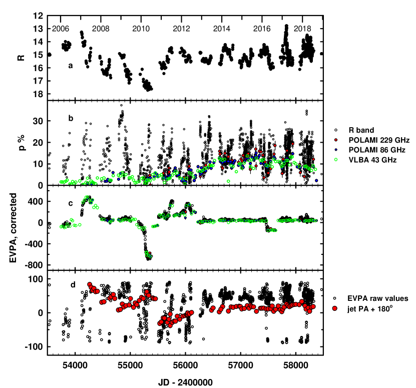
This high level of scatter of the optical PD is in striking contrast to the relatively smooth behaviour of the PD at radio frequencies; in fact, the radio PD mostly represents the lower envelope of the optical PD, as is seen in Figure 15(b). We propose that this contrast between optical and radio PD scatter is a consequence of very different volumes radiating at the two wavelength ranges in a plasma with a strong turbulent component of magnetic field: at radio frequencies the number of radiating cells with different magnetic field orientations is substantially larger than at optical bands, and the effect of each cell is diminished after vector co-addition of polarized intensity from all of the cells in the radiating volume. However, as seen in Figure 15(c), there is almost no difference in the direction of the electric vector position angle (EVPA) between optical and radio frequencies. At most epochs, this direction is parallel to the jet axis, strongly implying that a common process partially orders the magnetic field across the entire wavelength range, such as shocks or a helical field component. This ordering, superposed with the more chaotic field structure indicated by variability of the PD and sometimes the EVPA, agrees well with scenarios like the turbulent, extreme multi-zone model (TEMZ) developed by Marscher (2014).

In Figure 15 (d) we see a persistent offset between the mean optical EVPA and inner ($\lesssim 0.3$ mas) jet direction of $\sim 30^{\circ}$ starting in 2013. We note that the EVPA during this time interval is similar to the downstream (0.5-1.5 mas) jet direction of knots ejected prior to 2010 (see Table 3). This implies that the inner jet direction after mid-2013 might correspond to an elongated emission feature (e.g., a site of magnetic reconnections) oriented at an angle to the general jet flow. Given the strong projection effects, this angle can be as small as the angle at which we view the jet axis, $1.4$-$6^{\circ}$.

The large number of polarimetric measurements both in optical and radio bands allow us to look for minor differences between the EVPA behaviour at different wavelengths. To do this, in Fig. 16 we plot histograms of the EVPA distributions in optical $R$ band and radio frequencies of 229 GHz, 86 GHz, and 43 GHz. Unlike the plot in Fig. 15 (c), we constrain the range of EVPAs to $[-90,90]$ degrees. We immediately see a monotonic shift of the positions of maxima in the histograms with wavelength. We interpret this shift as a sign of Faraday rotation, and plot the values of these maxima relative to the square of wavelength in the bottom panel of the same figure. The values of the rotation measure (RM) obtained in this way for the pairs of frequencies $10^{5.6}$–229 GHz, 229–86 GHz, and 86–43 GHz are, correspondingly, $-35100\pm 3000,-7900\pm 1000$, and $-1900\pm 500$ rad$\cdot$m^-2. Neither the signs nor frequency dependence of the RM contradict earlier determinations (see, e.g., Kang et al., 2015; Park et al., 2018).

Figure 16: Top: Histograms of the EVPA distribution in optical and radio bands. Bottom: Positions of maxima of the 2014–2018 distributions vs. square of wavelength.

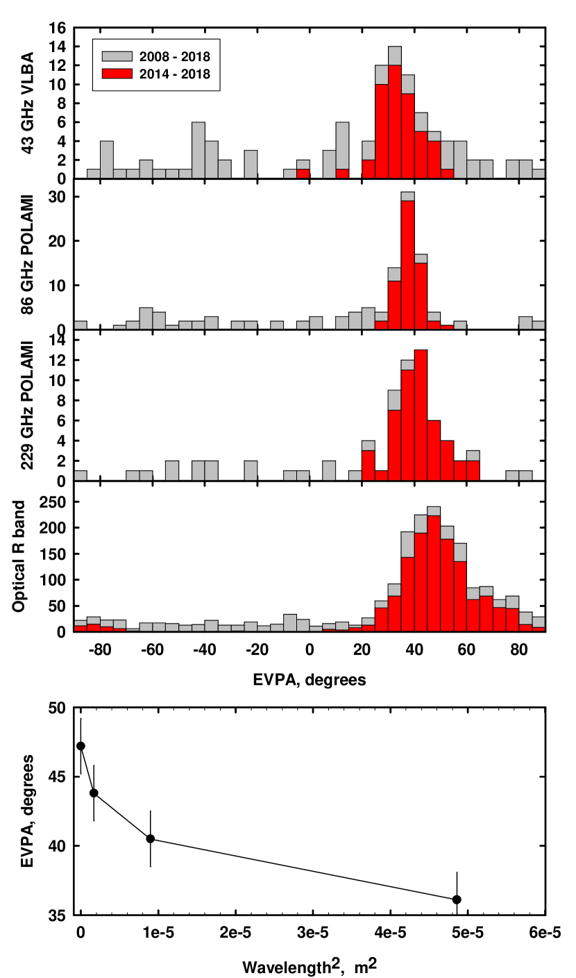
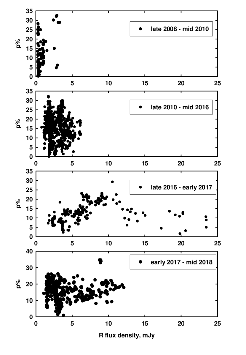
Figure 17 shows the dependencies of the optical PD on $R$-band flux density for different stages of activity (1)–(4), as defined in $ 3.6. The very different types of behaviour of PD vs. flux density may reflect different physical and geometrical conditions in the jet, as discussed above. Examples include changes in the Doppler factor due to shifts in viewing angle or variations in magnetic field strength and/or number of radiating electrons. Given the complexity of the observed behaviour, it is not surprising that time-limited campaigns may yield conclusions that are (or seem to be) contradictory.

Figure 17: Behaviour of fractional polarization of 3C 279 at different stages of activity.

Further important information that can be obtained from polarimetric data concerns possible spiral structure of the jet or helical structure of the magnetic field. During the past decade, several robust cases have been reported of optical EVPA rotations that mostly occurred close to optical, X-ray, and/or $\gamma$-ray outbursts, e.g., in BL Lac (Marscher et al., 2008), 3C 279 (Larionov et al., 2008), PKS 1510-089 (Marscher et al., 2010), S5 0716+71 (Larionov et al., 2013), and CTA 102 (Larionov et al., 2016b). However, regular patterns in the behaviour of polarization vector could also occur during quiescent states. Larionov et al. (2016a) suggested using a DCF analysis between normalized Stokes parameters $q$ and $u$ to uncover possible regular rotations that might be hidden by stochastic variability. If monotonic rotation of the EVPA is present during the temporal evolution of the polarization parameters, the curves of $q(t)$ and $u(t)$ must have a systematic shift relative to each other. In the opposite case, when only stochastic variability is present, no systematic shift is expected. Moreover, the direction of any rotation can be obtained from the sign of the DCF slope at lag=0: negative slope corresponds to counter-clockwise rotation and vice versa. In Fig. 18 we plot the DCF between $q$ and $u$ in optical $R$ band, which shows that during 2008–2018 there is a clear indication of anticlockwise rotation of the EVPA. To estimate the significance of the correlation between Stokes $q$ and $u$ parameters, we have performed a Monte-Carlo simulation in way similar to the one we used to estimate the significance of the $\gamma$-ray – optical correlation. The only difference is the method we used to make a set of synthetic curves. The time dependence of the Stokes parameters does not show well defined peaks, and cannot be adequately fit by a set of double exponential peaks, as is possible for the $\gamma$-ray and optical curves. To make synthetic light curves of the Stokes parameters, we approximated them using a damped random walk (DRW) model (Kelly et al., 2009; Zu et al., 2013). We used a JAVELIN code to obtain parameters of the DRW models for both $q$ and $u$ data sets and to generate $10^{4}$ random light curves with the derived parameters. By correlating these synthetic light curves, we find that the maximum difference of 0.4 between the highest-magnitude positive and negative correlations of the observed $q$ and $u$ data sets is reached only in $3\cdot 10^{-4}$ cases. Therefore, we can consider this correlation to be statistically significant at the 0.03 per cent level.

Figure 18: Discrete correlation function between normalized Stokes parameters $q$ and $u$ in optical $R$ band for the time interval 2008–2018 (top) and statistical distribution of the lag of the peak from Monte Carlo simulations (bottom). The grey area in the upper panel correspond to $\pm 1\sigma$ spread of simulated DCFs.

4 CONCLUSIONS

We have reported the results of decade-long (2008–2018) monitoring of the blazar 3C 279 from $\gamma$-rays to 1 GHz radio frequencies. Our data set includes Fermi and Swift data, obtained alongside an intensive GASP-WEBT collaboration campaign, polarimetric and spectroscopic data collected during the same time interval, and roughly monthly sequences of VLBA images at 43 GHz.

By analysing the multi-colour flux dependencies, we have isolated the spectra of the variable optical to near-IR continuum, which follows a power law with slope ranging from $-1.47$ to $-1.65$. Our multi-epoch optical spectra reveal changes in Mg ii and Fe ii emission-line flux. The Mg ii line consists of a component at the systemic redshift of 3C 279, as well as a second component 3500 km s^-1 on the long-wavelength (red) side. The fluxes of both components are proportional to the optical continuum flux, although the redder component has a stronger dependence. If the redder feature is free falling toward the central black hole, we estimate that the line-emitting clouds lie $\sim 0.6$ pc from the black hole. The reverberation of the changing continuum – which is synchrotron emission from the jet – is less than two months, restricting the location of the clouds to within $\sim 10\degr$ of the jet axis as viewed by the black hole. This polar line emission is likely to be a significant, variable source of seed photons for ‘external’ Compton scattering creating X-ray and $\gamma$-ray emission.

The SED contains the two-hump shape typical of blazars. The ratio of the higher peak, which falls in the $\gamma$-ray range, to the synchrotron peak in the IR, exceeds 100 during some outbursts. An analysis of the peak frequencies of the IR and $\gamma$-ray humps eliminates synchrotron self-Compton as the dominant $\gamma$-ray emission process during outbursts unless the magnetic field is extremely low, $\sim 0.4$ mG, and the plasma extremely far from equipartition between the magnetic and particle energy densities. Instead, EC emission appears to dominate at most epochs, which is consistent with the high $\gamma$-ray to IR-optical flux ratios.

The X-ray and $\gamma$-ray behaviour of 3C 279 are remarkably similar, with a time lag between the two light curves of $\la 3$ hours, indicating co-spatiality of the X-ray and $\gamma$-ray emission regions. The relation between the $\gamma$-ray and optical flux is quite complex, with a variety of slopes during different stages of activity. The dependence changes from linear to quadratic to a period when the $\gamma$-ray flux varied greatly during much more modest optical variations. At radio bands we have found progressive shifts of the most prominent light curve features with decreasing frequency, consistent with the emission peaking as it emerges from the $\tau=1$ surface. In addition, some fluctuations that emerge in the radio light curve disappear with decreasing frequency, which suggests different Doppler boosting of different radio-emitting zones in the jet.

From our series of VLBA images at 43 GHz, we have identified 14 bright knots that appear to move at various superluminal speeds. Some of the trajectories curve, with the direction of ‘ejection’ close to the ‘core’ changing with time. In 2010 two extremely bright knots initially emerged to the south-east of the core before veering toward the usual south-western direction of the $\ga 0.5$ mas-scale jet. Periods of different multi-wavelength behaviour of the light curves correspond to changes in the behaviour of the compact jet. The formation of three stationary emission features, which occurred after the direction of ejection became more consistent, and increase in apparent speed of moving knots up to $37c$ coincide with the highest-amplitude high-energy and optical outbursts. The extremely high apparent velocity requires a bulk Lorentz factor exceeding 37, which is nearly the value of $\sim 50$ needed to explain extremely rapid variations during the highest-amplitude $\gamma$-ray flares in 2013-15. Turbulent motions at the relativistic sound speed could increase this up to $\sim 70$ when a portion of the plasma moves toward the line of sight relative to the systemic flow.

The degree and position angle of linear polarization at optical and millimetre wavelengths (single-telescope and VLBA) changes with time, with the most rapid variability occurring at optical wavelengths. The correlation of variations in the optical $q$ and $u$ Stokes parameters corresponds to that expected in the case of a persistent helical magnetic field component or spiral motion of the radiating plasma.

The patterns of multi-wavelength variability of the flux, polarization, and structure of the relativistic jet of 3C 279 change over time. The variations in the ratios of the peak fluxes of the high-energy and optical-IR portions of the SED can be ascribed to changes in the ratio of the seed-photon to magnetic energy densities in the plasma frame. Such changes can occur via (1) variations in the bulk Lorentz factor of the plasma, (2) shifts in location of the site of acceleration of relativistic electrons relative to the emission-line clouds, especially those lying within $\sim 10^{\circ}$ of the jet axis, or (3) time-dependent reverberation of emission lines following variations in the UV continuum from either the jet or accretion disk. General variations of the flux can correspond to fluctuations in the number of radiating electrons, magnetic field (for synchrotron and SSC emission only), or Doppler factor, with the last of these caused by a variation in either the bulk Lorentz factor or direction of the velocity vector of the emitting plasma. The complexity of the variations in 3C 279 implies that most, or all, of these factors play a major role at different times.

AFFILIATIONS

¹Astron. Inst., St.-Petersburg State Univ., Russia
²Pulkovo Observatory, St.-Petersburg, Russia
³Institute for Astrophysical Research, Boston University, MA, USA
⁴INAF, Osservatorio Astrofisico di Torino, Italy
⁵Steward Observatory, University of Arizona, Tucson, AZ85721, USA
⁶ Instituto de Astrofísica de Andalucía-CSIC, Glorieta de la Astronomía s/n, E–18008 Granada, Spain
⁷Instituto de Astrofisica de Canarias (IAC), La Laguna, Tenerife, Spain
⁸ Departamento de Astrofisica, Universidad de La Laguna, La Laguna, Tenerife, Spain
⁹ University of Michigan, 323 West Hall, Dept of Astronomy, Ann Arbor MI, 48109-1107, USA
¹⁰ Institute of applied astronomy, Russian Academy of Sciences, Kutuzov  emb. 10 191187 St. Petersburg, Russia
¹¹ Institute of Astronomy and National Astronomical Observatory, Bulgarian Academy of Sciences, 72 Tsarigradsko shosse Blvd., 1784 Sofia, Bulgaria
¹² Astronomical Observatory, Department of Physical Sciences, Earth and Environment - University of Siena, Via Roma 56, 53100 Siena, Italy
¹³Crimean Astrophysical Observatory, Russia
¹⁴Dept. of Astronomy, Faculty of Physics, Sofia University, Bulgaria
¹⁵ Osservatorio Astronomico della Regione Autonoma Valle d’Aosta, I-11020 Nus, Italy
¹⁶EPT Observatories, Tijarafe, La Palma, Spain
¹⁷INAF, TNG Fundacion Galileo Galilei, La Palma, Spain
¹⁸ Max-Planck-Institut für Radioastronomie, Auf dem Hügel 69, 53121 Bonn, Germany
¹⁹ Graduate Institute of Astronomy, National Central University, Jhongli City, Taoyuan County 32001, Taiwan
²⁰Astronomical Observatory, Volgina 7, 11060 Belgrade, Serbia
²¹INAF, Osservatorio Astronomico di Roma, Italy
²² INAF - Osservatorio Astrofisico di Catania, via S. Sofia, 78, I-95123 Catania, Italy
²³ASI Italian Space Agency, Italy
²⁴ Center for Astrophysics $|$ Harvard & Smithsonian, 60 Garden Street, Cambrige, MA 02138 USA
²⁵ Finnish Centre for Astronomy with ESO, University of Turku, FI-20014 University of Turku, Finland
²⁶ Aalto University Metsähovi Radio Observatory, FI-02540 Kylmäl,̈ Finland
²⁷ Department of Physics and Astronomy, University of Shumen, 9700 Shumen, Bulgaria
²⁸ California Institute of Technology, 1216 E California Blvd, Pasadena, CA 91125, USA
²⁹Abastumani Observatory, Mt. Kanobili, 0301 Abastumani, Georgia
³⁰ Astro Space Center of Lebedev Physical Institute, Profsoyuznaya St. 84/32, 117997 Moscow, Russia
³¹ Institute of Physics and Technology, Dolgoprudny, Institutsky per., 9, Moscow region, 141700, Russia
³² Engelhardt Astronomical Observatory, Kazan Federal University, Tatarstan, Russia
³³ Landessternwarte, Zentrum für Astronomie der Universität Heidelberg, 69117 Heidelberg, Germany
³⁴ Aalto University Dept of Electronics and Nanoengineering, FI-00076 Aalto, Finland
³⁵Astronomical Institute, Osaka Kyoiku University, Osaka, 582-8582, Japan
³⁶ Special Astrophysical Observatory, Russian Academy of Sciences, Nizhnii Arkhyz, 369167 Russia
³⁷Kazan Federal University, 18 Kremlyovskaya St., Kazan, 420008, Russia
³⁸ Ulugh Beg Astronomical Institute, Uzbekistan Academy of Sciences, Astronomical street 33, Tashkent 100052, Uzbekistan
³⁹ INAF, Istituto di Radioastronomia, via Piero Gobetti 93/2, 40129 Bologna, Italy
⁴⁰Osservatorio Astronomico Sirio, Italy
⁴¹Department of Physics, University of Colorado, Denver, USA
⁴² Physical Research Laboratory, Navrangpura, Ahmedabad, Gujarat 380009, India
⁴³Institute of Astronomy, Bulgarian Academy of Sciences, Sofia, Bulgaria
⁴⁴ Instituto de Radio Astronomía Millimétrica, Avenida Divina Pastora, 7, Local 20, E–18012 Granada, Spain

References

- Abdo et al. (2010) Abdo A. A., et al., 2010, ApJ, 722, 520
- Ackermann et al. (2016) Ackermann M., et al., 2016, ApJ, 824, L20
- Agudo et al. (2010) Agudo I., Thum C., Wiesemeyer H., Krichbaum T. P., 2010, ApJS, 189, 1
- Agudo et al. (2014) Agudo I., Thum C., Gómez J. L., Wiesemeyer H., 2014, A&A, 566, A59
- Agudo et al. (2018a) Agudo I., Thum C., Ramakrishnan V., Molina S. N., Casadio C., Gómez J. L., 2018a, MNRAS, 473, 1850
- Agudo et al. (2018b) Agudo I., et al., 2018b, MNRAS, 474, 1427
- Aller et al. (1985) Aller H. D., Aller M. F., Latimer G. E., Hodge P. E., 1985, ApJS, 59, 513
- Arnaud (1996) Arnaud K. A., 1996, in Jacoby G. H., Barnes J., eds, Astronomical Society of the Pacific Conference Series Vol. 101, Astronomical Data Analysis Software and Systems V. p. 17
- Atwood et al. (2009) Atwood W. B., et al., 2009, ApJ, 697, 1071
- Baars et al. (1977a) Baars J. W. M., Genzel R., Pauliny-Toth I. I. K., Witzel A., 1977a, A&A, 61, 99
- Baars et al. (1977b) Baars J. W. M., Genzel R., Pauliny-Toth I. I. K., Witzel A., 1977b, A&A, 500, 135
- Böttcher et al. (2005) Böttcher M., et al., 2005, ApJ, 631, 169
- Böttcher et al. (2007) Böttcher M., et al., 2007, ApJ, 670, 968
- Bowker & Lieberman (1972) Bowker A. H., Lieberman G. J., 1972, Engineering Statistics. Prentice Hall, Inc.
- Burbidge & Rosenberg (1965) Burbidge E. M., Rosenberg F. D., 1965, ApJ, 142, 1673
- Carnerero et al. (2015) Carnerero M. I., et al., 2015, MNRAS, 450, 2677
- Cash (1979) Cash W., 1979, ApJ, 228, 939
- Chatterjee et al. (2008) Chatterjee R., et al., 2008, ApJ, 689, 79
- Corbin (1997) Corbin M. R., 1997, ApJ, 485, 517
- D’Ammando et al. (2012) D’Ammando F., et al., 2012, MNRAS, 426, 317
- Dermer (1995) Dermer C. D., 1995, ApJ, 446, L63
- Dickey & Lockman (1990) Dickey J. M., Lockman F. J., 1990, ARA&A, 28, 215
- Edelson & Krolik (1988) Edelson R. A., Krolik J. H., 1988, ApJ, 333, 646
- Fitzpatrick (1999) Fitzpatrick E. L., 1999, PASP, 111, 63
- Gaur et al. (2019) Gaur H., et al., 2019, MNRAS, 484, 5633
- Giannios et al. (2009) Giannios D., Uzdensky D. A., Begelman M. C., 2009, MNRAS, 395, L29
- González-Pérez et al. (2001) González-Pérez J. N., Kidger M. R., Martín-Luis F., 2001, AJ, 122, 2055
- Guerras et al. (2013) Guerras E., Mediavilla E., Jimenez-Vicente J., Kochanek C. S., Muñoz J. A., Falco E., Motta V., Rojas K., 2013, The Astrophysical Journal, 778, 123
- Hagen-Thorn et al. (2008) Hagen-Thorn V. A., Larionov V. M., Jorstad S. G., Arkharov A. A., Hagen-Thorn E. I., Efimova N. V., Larionova L. V., Marscher A. P., 2008, ApJ, 672, 40
- Hayashida et al. (2012) Hayashida M., et al., 2012, ApJ, 754, 114
- Hayashida et al. (2015) Hayashida M., et al., 2015, ApJ, 807, 79
- Hufnagel & Bregman (1992) Hufnagel B. R., Bregman J. N., 1992, ApJ, 386, 473
- Isler et al. (2015) Isler J. C., et al., 2015, ApJ, 804, 7
- Isler et al. (2017) Isler J. C., Urry C. M., Coppi P., Bailyn C., Brady M., MacPherson E., Buxton M., Hasan I., 2017, ApJ, 844, 107
- Jorstad & Marscher (2016) Jorstad S., Marscher A., 2016, Galaxies, 4, 47
- Jorstad et al. (2001a) Jorstad S. G., Marscher A. P., Mattox J. R., Wehrle A. E., Bloom S. D., Yurchenko A. V., 2001a, ApJS, 134, 181
- Jorstad et al. (2001b) Jorstad S. G., Marscher A. P., Mattox J. R., Aller M. F., Aller H. D., Wehrle A. E., Bloom S. D., 2001b, ApJ, 556, 738
- Jorstad et al. (2004) Jorstad S. G., Marscher A. P., Lister M. L., Stirling A. M., Cawthorne T. V., Gómez J.-L., Gear W. K., 2004, AJ, 127, 3115
- Jorstad et al. (2005) Jorstad S. G., et al., 2005, AJ, 130, 1418
- Jorstad et al. (2007) Jorstad S. G., et al., 2007, AJ, 134, 799
- Jorstad et al. (2010) Jorstad S. G., et al., 2010, ApJ, 715, 362
- Jorstad et al. (2017) Jorstad S. G., et al., 2017, ApJ, 846, 98
- Kang et al. (2015) Kang S., Lee S.-S., Byun D.-Y., 2015, J. Korean Astron. Soc., 48, 257
- Kelly et al. (2009) Kelly B. C., Bechtold J., Siemiginowska A., 2009, ApJ, 698, 895
- Khaikin et al. (1972) Khaikin S. E., Kaidanovskii N. L., Pariiskii I. N., Esepkina N. A., 1972, Izvestiya Glavnoj Astronomicheskoj Observatorii v Pulkove, 188, 3
- Kiehlmann et al. (2016) Kiehlmann S., et al., 2016, A&A, 590, A10
- Korolkov & Pariiskii (1979) Korolkov D. V., Pariiskii I. N., 1979, Sky & Telesc., 57, 324
- Kovalev et al. (1999) Kovalev Y. Y., Nizhelsky N. A., Kovalev Y. A., Berlin A. B., Zhekanis G. V., Mingaliev M. G., Bogdantsov A. V., 1999, A&AS, 139, 545
- Larionov et al. (2008) Larionov V. M., et al., 2008, A&A, 492, 389
- Larionov et al. (2010) Larionov V. M., Villata M., Raiteri C. M., 2010, A&A, 510, A93
- Larionov et al. (2013) Larionov V. M., et al., 2013, ApJ, 768, 40
- Larionov et al. (2016a) Larionov V., Jorstad S., Marscher A., Smith P., 2016a, Galaxies, 4, 43
- Larionov et al. (2016b) Larionov V. M., et al., 2016b, MNRAS, 461, 3047
- Larionov et al. (2017) Larionov V., et al., 2017, Galaxies, 5, 91
- León-Tavares et al. (2013) León-Tavares J., et al., 2013, ApJ, 763, L36
- León-Tavares et al. (2015) León-Tavares J., Chavushyan V., Lobanov A., Valtaoja E., Arshakian T. G., 2015, in Massaro F., Cheung C. C., Lopez E., Siemiginowska A., eds, IAU Symposium Vol. 313, Extragalactic Jets from Every Angle. pp 43–47, doi:10.1017/S1743921315001842
- Lister et al. (2016) Lister M. L., et al., 2016, AJ, 152, 12
- Lister et al. (2019) Lister M. L., et al., 2019, ApJ, 874, 43
- Lu et al. (2013) Lu R.-S., et al., 2013, ApJ, 772, 13
- MacDonald et al. (2015) MacDonald N. R., Marscher A. P., Jorstad S. G., Joshi M., 2015, ApJ, 804, 111
- MacDonald et al. (2017) MacDonald N. R., Jorstad S. G., Marscher A. P., 2017, ApJ, 850, 87
- Malmrose et al. (2011) Malmrose M. P., Marscher A. P., Jorstad S. G., Nikutta R., Elitzur M., 2011, ApJ, 732, 116
- Marscher (2014) Marscher A. P., 2014, ApJ, 780, 87
- Marscher & Gear (1985) Marscher A. P., Gear W. K., 1985, ApJ, 298, 114
- Marscher et al. (2008) Marscher A. P., et al., 2008, Nature, 452, 966
- Marscher et al. (2010) Marscher A. P., et al., 2010, ApJ, 710, L126
- Marscher et al. (2018) Marscher A. P., et al., 2018, The Astrophysical Journal, 867, 128
- Marziani et al. (1996) Marziani P., Sulentic J. W., Dultzin-Hacyan D., Calvani M., Moles M., 1996, ApJS, 104, 37
- Massaro et al. (2006) Massaro E., Tramacere A., Perri M., Giommi P., Tosti G., 2006, A&A, 448, 861
- Mead et al. (1990) Mead A. R. G., Ballard K. R., Brand P. W. J. L., Hough J. H., Brindle C., Bailey J. A., 1990, A&AS, 83, 183
- Mingaliev et al. (2014) Mingaliev M. G., Sotnikova Y. V., Udovitskiy R. Y., Mufakharov T. V., Nieppola E., Erkenov A. K., 2014, A&A, 572, A59
- Moretti et al. (2005) Moretti A., et al., 2005, in Siegmund O. H. W., ed., Proc. SPIEVol. 5898, UV, X-Ray, and Gamma-Ray Space Instrumentation for Astronomy XIV. pp 360–368, doi:10.1117/12.617164
- Nilsson et al. (2009) Nilsson K., Pursimo T., Villforth C., Lindfors E., Takalo L. O., 2009, A&A, 505, 601
- Parijskij (1993) Parijskij Y. N., 1993, IEEE Antennas and Propagation Magazine, 35, 7
- Park et al. (2018) Park J., et al., 2018, ApJ, 860, 112
- Patiño-Álvarez et al. (2018) Patiño-Álvarez V. M., et al., 2018, MNRAS, 479, 2037
- Peterson et al. (1998) Peterson B. M., Wanders I., Horne K., Collier S., Alexander T., Kaspi S., Maoz D., 1998, PASP, 110, 660
- Pittori et al. (2018) Pittori C., et al., 2018, ApJ, 856, 99
- Punsly (2013) Punsly B., 2013, ApJ, 762, L25
- Qian et al. (2019) Qian S. J., Britzen S., Krichbaum T. P., Witzel A., 2019, A&A, 621, A11
- Raiteri et al. (1998) Raiteri C. M., Villata M., Lanteri L., Cavallone M., Sobrito G., 1998, A&AS, 130, 495
- Raiteri et al. (2007) Raiteri C. M., et al., 2007, A&A, 473, 819
- Raiteri et al. (2008) Raiteri C. M., et al., 2008, A&A, 491, 755
- Raiteri et al. (2012) Raiteri C. M., et al., 2012, A&A, 545, A48
- Raiteri et al. (2017) Raiteri C. M., et al., 2017, Nature, 552, 374
- Rani et al. (2018) Rani B., et al., 2018, ApJ, 858, 80
- Richards et al. (2011) Richards J. L., et al., 2011, ApJS, 194, 29
- Rybicki & Lightman (1979) Rybicki G. B., Lightman A. P., 1979, Astronomy Quarterly, 3, 199
- Schlafly & Finkbeiner (2011) Schlafly E. F., Finkbeiner D. P., 2011, ApJ, 737, 103
- Shepherd (1997) Shepherd M. C., 1997, in Hunt G., Payne H., eds, Astronomical Society of the Pacific Conference Series Vol. 125, Astronomical Data Analysis Software and Systems VI. p. 77
- Sikora et al. (2009) Sikora M., Stawarz Ł., Moderski R., Nalewajko K., Madejski G. M., 2009, ApJ, 704, 38
- Smith et al. (2011) Smith P. S., Schmidt G. D., Jannuzi B. T., 2011, arXiv e-prints, p. arXiv:1110.6040
- Stocke et al. (1998) Stocke J. T., Penton S., Harvanek M., Neely W. A., Blades J. C., 1998, AJ, 115, 451
- Thum et al. (2008) Thum C., Wiesemeyer H., Paubert G., Navarro S., Morris D., 2008, PASP, 120, 777
- Thum et al. (2018) Thum C., Agudo I., Molina S. N., Casadio C., Gómez J. L., Morris D., Ramakrishnan V., Sievers A., 2018, MNRAS, 473, 2506
- Tsybulev (2011) Tsybulev P. G., 2011, Astrophysical Bulletin, 66, 109
- Udovitskiy et al. (2016) Udovitskiy R. Y., Sotnikova Y. V., Mingaliev M. G., Tsybulev P. G., Zhekanis G. V., Nizhelskij N. A., 2016, Astrophysical Bulletin, 71, 496
- Unwin et al. (1989) Unwin S. C., Cohen M. H., Biretta J. A., Hodges M. W., Zensus J. A., 1989, ApJ, 340, 117
- Vacca et al. (2003) Vacca W. D., Cushing M. C., Rayner J. T., 2003, PASP, 115, 389
- Vestergaard & Wilkes (2001) Vestergaard M., Wilkes B. J., 2001, ApJS, 134, 1
- Villata et al. (2002) Villata M., et al., 2002, A&A, 390, 407
- Villata et al. (2006) Villata M., et al., 2006, A&A, 453, 817
- Villata et al. (2008) Villata M., et al., 2008, A&A, 481, L79
- Villata et al. (2009) Villata M., et al., 2009, A&A, 504, L9
- Wardle & Kronberg (1974) Wardle J. F. C., Kronberg P. P., 1974, ApJ, 194, 249
- Wehrle et al. (1998) Wehrle A. E., et al., 1998, ApJ, 497, 178
- Wehrle et al. (2001) Wehrle A. E., Piner B. G., Unwin S. C., Zook A. C., Xu W., Marscher A. P., Teräsranta H., Valtaoja E., 2001, ApJS, 133, 297
- Wills & Brotherton (1995) Wills B. J., Brotherton M. S., 1995, ApJ, 448, L81
- Wood et al. (2017) Wood M., Caputo R., Charles E., Di Mauro M., Magill J., Perkins J. S., Fermi-LAT Collaboration 2017, International Cosmic Ray Conference, 35, 824
- Zu et al. (2013) Zu Y., Kochanek C. S., Kozłowski S., Udalski A., 2013, ApJ, 765, 106