Variational-Correlations Approach to Quantum Many-body Problems

Abstract

We investigate an approach for studying the ground state of a quantum many-body Hamiltonian that is based on treating the correlation functions as variational parameters. In this approach, the challenge set by the exponentially-large Hilbert space is circumvented by approximating the positivity of the density matrix, order-by-order, in a way that keeps track of a limited set of correlation functions. In particular, the density-matrix description is replaced by a correlation matrix whose dimension is kept linear in system size, to all orders of the approximation. Unlike the conventional variational principle which provides an upper bound on the ground-state energy, in this approach one obtains a lower bound instead. By treating several one-dimensional spin $1/2$ Hamiltonians, we demonstrate the ability of this approach to produce long-range correlations, and a ground-state energy that converges to the exact result. Possible extensions, including to higher-excited states are discussed.

I Introduction

Systems comprising of many interacting quantum particles are encountered in various fields, from condensed-matter and cold-atoms systems to quantum chemistry and nuclear matter. The ability to analyze quantum many-body systems, however, is severely limited by the exponential amount of information needed to describe the quantum wave-function. The challenge in studying quantum many-body systems is, therefore, to access the relevant physical observables without having to store and manipulate the full wave function

In one dimension (1d), the Density Matrix Renormalization Group (DMRG) method does that by employing the Matrix Product State representation that can describe ground states using an amount of information that scales only as a power law with the system size (and for gapped ground states strictly linear) (White, 1992, 1993; Schollwöck, 2005). This is not the case, however, for higher-dimensional systems or for highly-excited states. Quantum Monte Carlo simulations (Gubernatis et al., 2016) are not limited to 1d. However, they are only suitable for systems not suffering from the notorious “sign problem” (Loh et al., 1990), leaving out many interesting physical systems. Recently, promising results have been achieved by employing machine learning techniques to study quantum many-body systems (Carleo and Troyer, 2017; Melko et al., 2019; Sharir et al., 2019), and the full potential of these methods is yet to be discovered.

In this paper, we discuss a method for numerically studying the ground state of quantum many-body systems. This method relies on directly accessing a limited amount of physical information, involving the energy and several correlation functions, instead of treating the full quantum many-body wave function. This is done by treating these correlation functions as variational parameters in the minimization of the ground-state energy. Importantly, constraints are placed on the correlation functions, in a way that approximates the condition of the density-matrix being positive semidefinite. By gradually keeping more correlation functions, this approximation becomes increasingly better, and the resulting ground-state energy approaches its exact value.

Our approach follows a similar logic to that of the variational two-electron reduced density matrix (2-RDM) method (Mazziotti, 2002; Zhao et al., 2004; Mazziotti, 2005, 2006, 2007; Barthel and Hübener, 2012; Baumgratz and Plenio, 2012; Anderson et al., 2013; Verstichel et al., 2013; Mazziotti, 2016; Alcoba et al., 2018; Rubio-García et al., 2019), developed in the context of quantum chemistry. As in these past works, the method we discuss involves a relaxation of the constraints on the many-body wave-function, and it therefore yields a lower bound on the ground-state energy. In the present work, an emphasis is put on limiting the amount of information kept in a way that enables applying the approximation order by order, without changing the scaling of the computation with the system size. This allows for the treatment of large systems, including in the absence of translational invariance.

More specifically, this relaxation is achieved by substituting the density-matrix description of the system, which requires an exponentially-large amount of information, with a physical correlation matrix whose dimension is only linear in the system size. To demonstrate the variational-correlations approach, we treat several one-dimensional spin-1/2 models, with and without disorder, and show the method can achieve convergence towards the exact ground-state energy, as well as to produce long-range spin correlations.

II The variational correlations Approach

For simplicity, we present the formalism as it applies to spin-1/2 chains with nearest neighbor interactions. An extension to more general systems and higher dimensions is straightforward. The Hamiltonian for such a system is most generally given by

$$\hat{H}=\sum_{n=1}^{N}\sum_{i\in\{x,y,z\}}\sum_{\alpha\in\{0,x,y,z\}}J_{ni\alpha}\hat{\sigma}_{n}^{i}\hat{\sigma}_{n+1}^{\alpha},$$ (1)

where $N$ is the number of spins, $n$ runs over the chain’s sites, $\hat{\sigma}_{n}^{x,y,z}$ are the Pauli matrices on site $n$, and $\hat{\sigma}_{n}^{0}$ is the identity matrix on site $n$. The system is assumed to have periodic boundary conditions, namely $\hat{\sigma}_{N+1}^{\alpha}$ should be identified with $\hat{\sigma}_{1}^{\alpha}$.

II.1 The variational principle

We begin by formulating the conventional variational principle in terms of the density matrix. The density matrix for the system can most generally be written as

$$\hat{\rho}=\frac{1}{2^{N}}\sum_{\alpha_{1},\dots,\alpha_{N}}p_{\alpha_{1},\dots,\alpha_{N}}\hat{\sigma}_{1}^{\alpha_{1}}\hat{\sigma}_{2}^{\alpha_{2}}\dots\hat{\sigma}_{N}^{\alpha_{N}},$$ (2)

where each of the indices $\alpha_{n}$ runs over $0,x,y,z$. In this representation the density matrix is parameterized by the tensor $p_{\alpha_{1},\dots,\alpha_{N}}$, which contains $4^{N}$ elements. For $\hat{\rho}$ to be a valid density matrix it must obey $\rho=\rho^{\dagger},$ ${\rm Tr}(\rho)=1$, and $\rho\succeq 0$ (positive semidefiniteness). The first two conditions are enforced by $p_{\alpha_{1},\dots,\alpha_{N}}=p_{\alpha_{1},\dots,\alpha_{N}}^{\ast}$ and $p_{0,\dots,0}=1$, respectively.

The variational principle states that the ground state of $\hat{H}$ is described by the parameters, $p_{\alpha_{1},\dots,\alpha_{N}}^{{\rm gs}}$, satisfying

$$\begin{split}\underset{\{p\}}{{\rm minimize}}\,\,&E(\{p\})={\rm Tr}(\hat{\rho}\hat{H})\\ {\rm s.t.}\hskip 10.00002pt&\hskip 10.00002pt\hat{\rho}(\{p\})\succeq 0.\end{split}$$ (3)

In the absence of ground-state degeneracy, the resulting density matrix is guaranteed to describe a pure state, while in the case of a degenerate ground state it can more generally describe a classical mixture of several ground states.

For a large system, obtaining $p_{\alpha_{1},\dots,\alpha_{N}}^{{\rm gs}}$ through a straight-forward numerical minimization is impractical due to the exponentially-large number of parameters in $\{p\}$. Notice, however, that the function to be minimized, $E(\{p\})$, only involves a small subset of the elements in $\{p\}$. Specifically, it contains those elements that have the form

$${\rm Tr}(\hat{\rho}\hat{\sigma}_{n}^{i}\hat{\sigma}_{n+1}^{\alpha})=p_{\underset{1}{0},0,\dots,0,\underset{n}{i},\alpha,0,\dots,\underset{N}{0}},$$ (4)

whose number scales linearly with the system size, $N$. Instead, it is the condition $\hat{\rho}\succeq 0$ that limits the application of the variational principle by coupling this subset with the rest of the parameters in $\{p\}$.

With this in mind, we now look for a condition that would approximate $\hat{\rho}\succeq 0$ in a manner involving only a subset of parameters in $\{p\}$. More specifically, we shall formulate an ordered approximation to $\hat{\rho}\succeq 0$ that invokes a number of parameters scaling quadratically in $N$, for any order of the approximation (and linearly in $N$ for translationally-invariant systems).

II.2 Approximating the positive-semidefiniteness condition

To approximate the condition $\hat{\rho}\succeq 0$, we rely on the observation that $\hat{\rho}\succeq 0$ if and only if

$${\rm Var}(\hat{O}) =\langle(\hat{O}-\langle\hat{O}\rangle)^{2}\rangle\geq 0$$ (5)

for any hermitian operator $\hat{O}$, where $\left\langle\cdot\right\rangle\equiv{\rm Tr}(\hat{\rho}\,\cdot)$. The forward direction easily follows from noting that ${\rm Var}(\hat{O})={\rm Tr}(\hat{\rho}\hat{A})$ where $\hat{A}=[\hat{O}-{\rm Tr}(\hat{\rho}\hat{O})]^{2}$ is positive semidefinite, because it is the square of a Hermitian operator. Together with $\hat{\rho}\succeq 0$ this readily ensures ${\rm Var}(\hat{O})\geq 0$.

To prove the converse direction, let us denote by $\{|l\rangle,w_{l}\}_{l}$ the set of eigenstates and eigenvalues of $\hat{\rho}$. If ${\rm Var}(\hat{O})\geq 0$ for any hermitian $\hat{O}$, it is in particular true for $\hat{O}=\left|l\right\rangle\left\langle l\right|$, from which it follows that

$$0\leq{\rm Var}(\left|l\right\rangle\left\langle l\right|)=w_{l}(1-w_{l}),$$ (6)

namely $0\leq w_{l}\leq 1$. Since this is true for any $l$, one concludes that all the eigenvalues of $\hat{\rho}$ are non-negative, i.e. $\hat{\rho}\succeq 0$.

The equivalence between $\hat{\rho}\succeq 0$ and Eq. (5) suggests a route towards approximating the condition $\hat{\rho}\succeq 0$. Instead of requiring that all hermitian operators have a non-negative variance, let us limit this requirement to the subset of hermitian operators that have the form

$$\hat{O}^{(k)}=\sum_{n,\nu}c_{n\nu}\hat{L}_{n,\nu}^{(k)},$$ (7)

where $c_{n\nu}$ are real coefficients and $\{\hat{L}_{n,\nu}^{(k)}\}_{\nu=1}^{3\times 4^{k-1}}$ span the space of range-$k$ local hermitian zero-trace operators, that is

$$\begin{split}\{\hat{L}_{n,\nu}^{(1)}\}_{\nu}&=\{\hat{\sigma}_{n}^{i}\}_{i}\,\,\,;\,\,\,\{\hat{L}_{n,\nu}^{(2)}\}_{\nu}=\{\hat{\sigma}_{n}^{i}\hat{\sigma}_{n+1}^{\alpha}\}_{i,\alpha}\,\,\,;\\ \{\hat{L}_{n,\nu}^{(3)}\}_{\nu}&=\{\hat{\sigma}_{n}^{i}\hat{\sigma}_{n+1}^{\alpha}\hat{\sigma}_{n+2}^{\beta}\}_{i,\alpha,\beta}\,\,\,;\,\,\,\dots\end{split}$$ (8)

where $i\in\{x,y,z\}$ and $\alpha,\beta\in\{0,x,y,z\}$. As $k$ increases, the condition ${\rm Var}(\hat{O}^{(k)})\geq 0$ becomes a better approximation of $\hat{\rho}\succeq 0$. While the two conditions are strictly equivalent only when $k=N$, we shall see below that it is often sufficient to consider the case $k=2$ or $k=3$.

The benefit of using the condition ${\rm Var}(\hat{O}^{(k)})\geq 0$ instead of the exact condition, $\hat{\rho}\succeq 0$, is that it can be enforced by constraining a relatively small set of the parameters, whose number scales only quadratically with the system size, $N$. To see this, let us substitute the expression for $\hat{O}^{(k)}$, Eq. (7), in the condition ${\rm Var}(\hat{O}^{(k)})\geq 0$. This results in the condition

$$\sum_{m,n,\mu,\nu}c_{m\mu}\mathcal{M}_{m\mu,n\nu}^{(k)}c_{n\nu}\geq 0\hskip 10.00002pt\forall\,\,\{c_{n\nu}\},$$ (9)

where

$$\begin{split}\mathcal{M}_{m\mu,n\nu}^{(k)}\equiv\frac{1}{2}&\langle\{\hat{L}_{m\mu}^{(k)},\hat{L}_{n\nu}^{(k)}\}\rangle-\langle\hat{L}_{m\mu}^{(k)}\rangle\langle\hat{L}_{n\nu}^{(k)}\rangle,\end{split}$$ (10)

is the correlation matrix considered in Ref. (Qi and Ranard, 2019), which is manifestly real and symmetric. Here, $\{\cdot,\cdot\}$ stands for the anticommutator. The condition, Eq. (9), is equivalent to $\mathcal{M}^{(k)}\succeq 0$. We thus approximate the condition that $\hat{\rho}$ is positive semidefinite by the condition that the correlation matrix, $\mathcal{M}^{(k)}$, is positive semidefinite. Importantly, while the dimension of $\hat{\rho}$ is $d_{\rho}=2^{N}$, making it intractable, the dimension of $\mathcal{M}^{(k)}$ is $d_{\mathcal{M}}=3\cdot 4^{k-1}N$.

Had we not limited the range of the operators $\hat{L}^{(k)}$ in Eq. (7), the resulting constraint would be equivalent to the so-called $k$-positivity conditions (Mazziotti and Erdahl, 2001), which require that all $k$-body reduced density matrices (RDM) are positive-semidefinite, and which are at the source of the variational 2-RDM method (Mazziotti, 2002; Zhao et al., 2004; Mazziotti, 2005, 2006, 2007; Barthel and Hübener, 2012; Baumgratz and Plenio, 2012; Anderson et al., 2013; Verstichel et al., 2013; Mazziotti, 2016; Alcoba et al., 2018; Rubio-García et al., 2019). The dimension of the $k$-body RDM scales as $N^{k}$, which typically limits the ability to increase accuracy by increasing $k$. In contrast, by restricting the range of $\hat{L}^{(k)}$ to be $k$, we force the dimension of the correlation matrix $\mathcal{M}^{(k)}$ to remain linear in $N$ for any fixed $k$. In this regard, one should also note Ref. (Barthel and Hübener, 2012), where restrictions on the range of considered operators are placed using a different protocol, enabling the authors to treat both 1d and 2d lattice systems. Finally, note that although the range $\hat{L}^{(k)}$ is restricted to $k$, the matrix $\mathcal{M}^{(k)}$ contains also long-range correlations since $m$ and $n$ in Eq. (10) are not restricted.

II.3 The variational-correlation procedure

We are now in a position to describe the variational-correlation procedure for approximating the system’s ground-state. We define the variational parameters as the disconnected correlation functions

$$b_{n\nu}\equiv\langle\hat{L}_{n\nu}^{(k)}\rangle\,\,\,\,;\,\,\,\,C_{m\mu n\nu} \equiv\langle\hat{L}_{m\mu}^{(k)}\hat{L}_{n\nu}^{(k)}\rangle\,\>{\rm for}\,\,(n\geq m+k),$$ (11)

collectively denoted by $x=\{b_{n\nu},C_{\mu\nu}^{mn}\}$, whose number scales quadratically with $N$. The approximate ground-state energy and correlations are then obtained “to order $k$” by solving the following optimization problem:

$$\begin{split}&\underset{\{x\}}{{\rm minimize}}\,\,\,E(\{x\})={\rm Tr}(\hat{\rho}\hat{H}),\\ &{\rm s.t.}\hskip 10.00002pt\mathcal{M}^{(k)}(\{x\})\succeq 0.\end{split}$$ (12)

The resulting energy, $E(\{x_{{\rm min}}\})$, sets a lower bound on the true ground-state energy of the system. This is because the constraint in Eq. (12) is a result of relaxing the constraint in the original minimization problem of Eq. (3). Namely, the minimum point of Eq. (3), which describes the exact ground state, is contained within the space of feasible points considered in the minimization problem of Eq. (12). Alternatively stated, unlike the conventional use of the variational principle where one places additional constrains on the wave function, here one relaxes the constraints on it (by replacing $\hat{\rho}\succeq 0$ with $\mathcal{M}^{(k)}\succeq 0$). While the former procedure yields an energy which is greater than the ground state, the latter yields an energy which is lower.

This, of course, comes at a price. First, we do not possess all the information about the ground state, but rather only correlation functions of the form given in Eq. (11). Second, the resulting ground state is generally not physical. In other words, the correlation functions $x_{{\rm min}}=\{b,C\}_{{\rm min}}$ cannot arise from an exactly positive semidefinite $\hat{\rho}$. Nevertheless, as $k$ increases these correlations should approximate the true ground-state correlation functions with increasing accuracy. In Sec. III, we demonstrate this method up to order $k=3$.

II.4 Interpretation of active constraints

Since the objective function in Eq. (12) is linear, the minimum point is always at the boundary of the region defined by $\mathcal{M}^{(k)}\succeq 0$. Namely, at the optimum, at least some of the eigenvalues of $\mathcal{M}^{(k)}$ are zero; these represent the active constraints of the problem. Each such zero eigenvalue of $\mathcal{M}^{(k)}$ corresponds to an eigenvector, with elements $\omega_{n\nu}$, which can be used to define an operator $\hat{\Omega}\in\hat{O}^{(k)}$,

$$\hat{\Omega}=\sum_{n,\nu}\omega_{n\nu}\hat{L}_{n\nu}^{(k)}.$$ (13)

Each such operator then obeys

$$\langle\hat{\Omega}^{2}\rangle-\langle\hat{\Omega}\rangle^{2}=\sum_{m,n,\mu,\nu}\omega_{m\mu}\mathcal{M}_{m\mu,n\nu}^{(k)}\omega_{n\nu}=0,$$ (14)

due to $\omega_{mn}$ being in the null space of $\mathcal{M}_{m\mu,n\nu}^{(k)}$. From Eq. (14), one infers that the ground state is an eigenstate of $\hat{\Omega}$. This could suggest that the accuracy of the variational correlation approximation is determined by the locality of the operators for which the ground-state is an eigenstate. If these operators can be approximated by operators in $\hat{O}^{(k)}$, they would manifest as active constraints in the minimization of Eq. (12), forcing the energy to increase and thereby get closer to the exact ground state energy.

II.5 Translational Invariance

The variational procedure described above can be significantly simplified when the Hamiltonian of Eq. (1) is translationally-invariant, namely when $J_{ni\alpha}$ is independent of $n$. In this case, the ground state (and in fact any eigenstate) of $\hat{H}$ is guaranteed to either be translationally invariant or degenerate. In the latter case one can always choose a superposition (or a classical mixture) of the degenerate ground states that would itself be translationally invariant.

We can, therefore, impose translational invariance on the variational correlations,

$$C_{m\mu;n\nu} =C_{\mu\nu}^{\left(n-m\right)}\hskip 10.00002pt;\hskip 10.00002ptb_{n\nu}=b_{\nu}.$$ (15)

This reduces the number of variational parameters, now denoted by $x=\{b_{\nu},C_{\mu\nu}^{\Delta n}\}$. In particular, the number of elements in $x$ scales only linearly with $N$.

III Numerical Results

In this section, we demonstrate the application of the variational correlation (VC) approximation, as defined in Eq. (12), for studying 1d Hamiltonians of nearest-neighbor interacting spin-$1/2$ particles. We focus on two types of models: (i) the tilted-field Ising model and (ii) the XXZ model.

We begin by examining the results for the ground state energy within the $k=2$ order of the approximation. These results are compared with those obtained from the density matrix renormalization group (DMRG), which for the studied systems are essentially exact. Next, the error within the $k=2$ order is examined as a function of the systems size and upon introducing disorder. We then study the dependence of the ground-state energy on $k$ by comparing results for $k=1,2,3$. Finally, we examine the results for the correlation functions. Details regarding the numerical implementation of the VC approximation are found in Appendix A.

III.1 Ground-state energy

III.1.1 Tilted-field Ising model

The Ising model with a tilted-filed is described by the Hamiltonian

$$\hat{H}_{{\rm Ising}}=\sum_{n=1}^{N}\left(h_{x}\hat{\sigma}_{n}^{x}+h_{z}\hat{\sigma}_{n}^{z}+J_{z}\hat{\sigma}_{n}^{z}\hat{\sigma}_{n+1}^{z}\right),$$ (16)

where periodic boundary conditions are assumed. This Hamiltonian is a special case of the Hamiltonian considered in Eq. (1). The direction of the field in the $xz$ plane is parameterized by the angle, $\theta,$ where $h_{x}=|\vec{h}|\cos\theta$ and $h_{z}=|\vec{h}|\sin\theta$.

(a)

(b)

Figure 1: Ground-state energy of the Ising model [see Eq. (16)] within the variational-correlations (VC) approximation, to order $k=2$, as a function of the field $|\vec{h}|$. The system size is $N=80$ spins. The VC method sets a lower-bound on the exact ground state energy of the system. In (a), the field angle is $\theta=0$, allowing for an exact analytical solution (solid blue line) by virtue of the Jordan Wigner transformation. In (b), the field angle is $\theta=\pi/6$ and results are compared with a density matrix renormalization group (DMRG) calculation (blue squares). Results are also compared with a mean-filed calculation (dashed black line), which sets an upper bound on the ground state energy.

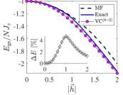
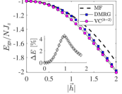
In Figs. 1(a) and  1(b), we present the ground-state energy for $\theta=0$ and $\theta=\pi/6$, respectively, calculated using the VC approximation to order $k=2$, for a system of $N=80$ spins. The results are shown as a function of the field strength, $|\vec{h}|$, for fixed $J_{z}=1$. In the case of $\theta=0$, the Hamiltonian can be solved exactly by mapping the problem to a system of free fermions by virtue of the Jordan-Wigner transformation (Suzuki et al., 2012). This solution is marked by a solid blue line in Fig. 1(a). As can be seen, the VC approximation is in reasonable agreement with the exact solution already in the $k=2$ order. Notice the maximal discrepancy is at $|\vec{h}|=J_{z},$ where the system is known to go through a continuous phase transition.

For a general field angle, an exact analytical calculation is not possible. Accordingly, the results of the VC approximation for the case of $\theta=\pi/6$, shown in Fig. 1(b), are compared with those of a DMRG calculation. The latter is implemented using the iTensor library (ITe, ). The results are qualitatively similar to those obtained for $\theta=0$. Importantly, we see that deviating from integrability does not reduce the accuracy of the approximation.

As explained in Sec. II.3, the variational correlation approximation sets a lower bound on the ground-state energy, contrary to the conventional variational principle which allows one to obtain an upper bound. This is manifested in comparing the results with those of a mean-field calculation. The latter is obtained by considering a product-state trial variational wave function, $|\Psi_{{\rm MF}}\rangle$, and minimizing $\langle\Psi_{{\rm MF}}|\hat{H}|\Psi_{{\rm MF}}\rangle$. Indeed, the mean-field result (dashed black line) bounds the exact result from above, while the VC approximation bounds it from below.

III.1.2 The XXZ model

The Hamiltonian describing the XXZ model is given by

$$\hat{H}_{{\rm XXZ}}=\sum_{n=1}^{N}\left[J_{x}\left(\hat{\sigma}_{n}^{x}\hat{\sigma}_{n+1}^{x}+\hat{\sigma}_{n}^{y}\hat{\sigma}_{n+1}^{y}\right)+J_{z}\hat{\sigma}_{n}^{z}\hat{\sigma}_{n+1}^{z}\right],$$ (17)

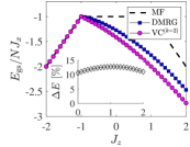
where, as before, periodic boundary conditions are assumed. The results for the ground-state energy as a function of the field $J_{z}$ are shown in Fig. 2(a) for fixed $J_{x}=1$ and $N=80$. As before, we compare the variational correlation method, calculated to order $k=2$, with the result of the variational mean-field state (dashed black line) and of the DMRG calculation (blue squares).

For $J_{z}<-1$, the ground state is a symmetry-broken ferromagnetic state with all spins pointing in the $z$ direction, and the energy is, therefore, linear in $J_{z}$. In this phase the VC, DMRG, and mean-field calculations all coincide. At $J_{z}=-1$, a first-order quantum phase transition occurs signalled by the discontinuous derivative of the ground-state energy. For $J_{z}>-1$, the results of the VC calculation start to deviate considerably from the DMRG result. In Sec. III.4 we shall see that this discrepancy can be mitigated by increasing the approximation order to $k=3$.

(a)

(b)

Figure 2: (a) Ground-state energy of the XXZ model with $N=80$ spins [see Eq. (17)], within the variational-correlations (VC) approximation, calculated to order $k=2$. Results are compared with a DMRG calculation (blue squares) and with a mean-filed calculation (dashed black line). At $J_{z}=-1$, the system goes through a first-order quantum phase transition, above which a discrepancy of up to $\sim 12\%$ develops between the VC and the DMRG results. (b) Difference between the ground-state energy calculated by DMRG and by the VC method to order $k=2$, as a function of system size, $N$, for fixed $J_{x}=1$ and different values of $J_{z}$. Notice the error does not increase with system size. As shown below, in Fig. 4, this error of the VC approximation decreases significantly upon going to the $k=3$ order.

III.2 Scaling of the error with system size

Before moving on to study the effect of increasing the order of approximation, $k$, it is important to examine the error of the VC approximation as a function of the system size, for a fixed value of $k$.

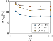
In Fig. 2(b), we present the relative energy difference $\Delta E=(E_{{\rm dmrg}}-E_{{\rm vc}})/|E_{{\rm dmrg}}|$ between the DMRG result and the VC approximation, calculated to order $k=2$, as a function of the number of spins, $N$, for the XXZ model of Eq. (17). Results are shown for several different values of $J_{z}$. Importantly, the relative error in energy does not increase with system size but rather goes to a constant.

III.3 Disorder

Next, let us examine the effect of introducing a disordered field. This is done by adding a term

$$\hat{H}_{{\rm dis}}=\sum_{n=1}^{N}h_{n}^{{\rm dis}}\hat{\sigma}_{n}^{z},$$ (18)

to the Hamiltonians of Eqs. (16) and (17), where $h_{n}^{{\rm dis}}\in[-W_{{\rm dis}},W_{{\rm dis}}]$ is a uniformly distributed random variable and $N=80$.

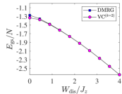
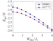
In Fig. 3, the ground-state energy is presented as a function of the disorder strength, $W_{{\rm dis}}$, for a single disorder realization, calculated using both DMRG and the VC approximation to order $k=2$. Figure 3(a) shows results for the transverse-field Ising model at its critical point, $h_{x}=J_{z}$, and Fig. 3(b) shows results for the Heisenberg model, obtained by setting $J_{x}=J_{z}$ in Eq. (17).

Increasing the strength of disorder actually improves the performance of the VC method at predicting true ground-state energies (i.e. the DMRG result) in both models. This could be related to the localization induced by the disorder field (see also the discussion in Sec. II.4).

(a)

(b)

Figure 3: Effect of a disorder field in the $z$ direction. The ground-state energy is plotted versus the disorder strength, as defined below Eq. (18), for (a) the transverse-field Ising model at its critical point, $h_{x}=J_{z}$, and (b) the Heisenberg model, $J_{x}=J_{z}$. The plots correspond to a single disorder realization. For both models, the variational correlation (VC) approximation becomes better as the disorder strength increases. Here, the system size was taken to be $N=80$.

III.4 Dependence on approximation order

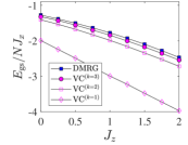
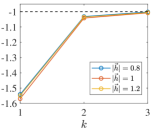
We now study the dependence of the VC approximation on the order of approximation, $k$. We examine first the XXZ model, for which the $k=2$ results were presented in Fig. 2. In Fig. 4(a), we present the results for the ground state energy with $N=30$ spins, calculated within the VC approximation to orders $k=1,2,3$. As $k$ increases, the energy approaches the DMRG results, shown in blue squares. This is emphasized in Fig. 4(b) which presents the VC ground state energy, $E_{{\rm vc}}$, normalized by $E_{{\rm dmrg}}$, for three values of $J_{z}$ as a function of $k$.

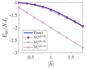
Similarly, In Figs. 4(c,d) the ground-state energy for the transverse-field Ising model ($\theta=0$) with $N=30$ spins is examined for three different approximation orders, $k=1,2,3$. Qualitatively similar behavior as in the XXZ model is observed, although with a faster convergence.

(a)	(b) $E_{\rm vc}^{(k)}/E_{\rm dmrg}$
(c)	(d) $E_{\rm vc}^{(k)}/E_{\rm exact}$

Figure 4: (a) Ground-state energy within the variational correlation (VC) approximation for the XXZ model with $N=30$ spins, for different values of the approximation order, $k=1,2,3$, with fixed $J_{x}=1$. Upon increasing $k$, the VC results approach those of the DMRG calculation, shown in blue squares. In (b), the energy is plotted as a function of $k$, for several values of $J_{z}$. Similar behavior is observed for the the transverse-field Ising model in (c) and (d).

III.5 Correlation functions

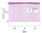
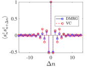
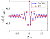
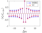
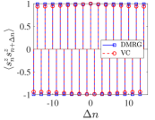
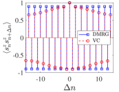
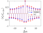
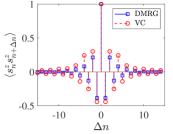
The VC approach, as described in Sec. II.3, allows for obtaining not only the ground-state energy but also correlation functions of the form $C_{m\mu n\nu}\equiv\langle\hat{L}_{m\mu}^{(k)}\hat{L}_{n\nu}^{(k)}\rangle$. We now examine the correlation functions obtained from the VC approximation, focusing on $k=3$, for which $\hat{L}_{n;i\alpha\beta}^{(k=3)}\equiv\hat{\sigma}_{n}^{i}\hat{\sigma}_{n+1}^{\alpha}\hat{\sigma}_{n+2}^{\beta}$.

In Fig. 5, we present the $\langle\hat{\sigma}_{n}^{z}\hat{\sigma}_{n+\Delta n}^{z}\rangle$ correlations for the XXZ model studied in Figs. 4(a,b), for several values of $J_{z}$, obtained from the $k=3$ order of the VC approximation. As before, the results are compared with those of a DMRG calculation. The VC method captures correctly the qualitative ferromagnetic [Fig. 5(a)] and antiferromagnetic correlations [Fig. 5(b-d)]. For small $\Delta n$, good quantitative agreement is observed. However, that slightly diminishes when increasing $\Delta n$. The same level of agreement is obtained when examining other kinds of spin-spin correlations (e.g. $\langle\hat{\sigma}_{m}^{x}\hat{\sigma}_{n}^{x}\rangle$). Similar conclusions can be drawn from Fig. 6, which presents the $\langle\sigma_{n}^{z}\sigma_{n+\Delta n}^{z}\rangle$ correlations for the transverse-field Ising model, for several fixed values of $|\vec{h}|$.

(a)	(b)
(c)	(d)

Figure 5: Correlation functions for the XXZ model with $N=30$ spins, calculated to order $k=3$ (red circles) and compared with DMRG (blue squares), for (a) $J_{z}=-2$, (b) $J_{z}=0.5$, (c) $J_{z}=1,$ and (d) $J_{z}=1.5$.

(a)	(b)
(c)	(d)

Figure 6: Correlation functions for the transverse-field Ising model with $N=30$ spins. Results are shown for the $k=3$ order of the VC approximation (red circles) and for DMRG (blue squares), for (a) $|\vec{h}|=0.2$, (b) $|\vec{h}|=0.6$, (c) $|\vec{h}|=1$, and (d) $|\vec{h}|=1.4$. These correspond to the ordered, critical, and disordered phases of the Ising model, respectively.

IV Discussion

We have investigated the variational correlations (VC) approach for studying the ground state of interacting many-body systems. In this approach, the elements of a correlation matrix, whose dimension is linear in system size, serve as the variational parameters, and replace the density matrix in describing the system. The variational procedure then relies on using this correlation matrix for obtaining an order-by-order approximation of the positive semidefiniteness condition of the density matrix. Since in this variational procedure one relaxes the constraint on the density matrix rather than over-constraining it, the resulting energy sets a lower bound on the true ground state energy, similar to the variational 2-RDM method (Mazziotti, 2002; Zhao et al., 2004; Mazziotti, 2005, 2006, 2007; Barthel and Hübener, 2012; Baumgratz and Plenio, 2012; Anderson et al., 2013; Verstichel et al., 2013; Mazziotti, 2016; Alcoba et al., 2018; Rubio-García et al., 2019).

The VC approach was tested on several 1d systems of spin 1/2 particles by comparing its results with those of DMRG, which for 1d systems is essentially exact. It was demonstrated that the VC approach is able to produce long-range correlations, as well as to provide a lower bound on the ground-state energy that converges to the exact result as the order of approximation is increased. Interestingly, the VC approximation becomes better in the presence of disorder. The fact that the VC approach provides a lower bound could be used together with a conventional variational ansatz (e.g. mean field) to bound the ground state energy from both above and below.

In 1d, the VC method offers no advantage over DMRG in terms of computational complexity, as both of them scale polynomially , and for a gapped system DMRG scales linearly. In 2d, however, DMRG scales exponentially with the width of the system (Stoudenmire and White, 2012), while the VC method remains polynomial. It will, therefore, be interesting to examine the VC approach when applied to models in 2d, where it has the potential to address some outstanding challenges, both in condensed matter and in cold atoms systems. Since the VC approximation can be formulated as an Semidefinite Programming (Vandenberghe and Boyd, 1996) (SDP) problem, recent advances (Yurtsever et al., 2017) in large-scale SDP algorithms could help to achieve this goal, as well as to attend higher-approximation orders. Interestingly, it has been suggested that SDP is one of a few problems that could acquire a speedup from the introduction of Noisy Intermediate-Scale Quantum (NISQ) technology (Preskill, 2018), through a recently-introduced algorithm dubbed Quantum Semidefinite Programming (Brandao and Svore, 2017; Van Apeldoorn et al., 2017; Brandão et al., 2019).

As explained in Sec. II.2, the VC approach is based on relaxing the condition of Eq. (5), by requiring it is obeyed for only a subset of operators, denoted $\hat{O}^{(k)}$, of range $k$-local operators. Clearly, one can choose a different subset of operators, amounting to a different way of approximating the ground state. Two such examples are the approximations employed in Refs. (Mazziotti, 2002; Zhao et al., 2004; Mazziotti, 2005, 2006, 2007; Baumgratz and Plenio, 2012; Anderson et al., 2013; Verstichel et al., 2013; Mazziotti, 2016; Alcoba et al., 2018; Rubio-García et al., 2019) and Ref. (Barthel and Hübener, 2012). It will therefore be interesting to study the effect of choosing different subsets of operators in Eq. (7), and the physical meaning of their resulting approximations. In particular, it is reasonable to assume that the optimal choice could depend on the properties of the ground-state being targeted.

Finally, while the VC method targets the ground-state, a possible extension might be to study excited states. This could possibly be achieved using the fact that the variance of the energy, $\langle H^{2}\rangle-\langle H\rangle^{2}$, which is a linear function of the correlation matrix, is a non-negative quantity that vanishes only for eigenstates. Minimizing it, while constraining $\langle H\rangle$ to lie withing a narrow window, could potentially yield an approximation for the correlation functions at finite energy density.

Appendix A Implementation

To numerically solve the minimization problem of Eq. (12), we first formulate it as a semidefinite programming (SDP) problem (Vandenberghe and Boyd, 1996). To this end we write the correlation matrix, defined in Eqs. (10) and (11), as

$$\mathcal{M}_{m\mu;n\nu}^{(k)}=C_{m\mu;n\nu}-b_{m\mu}b_{n\nu,}$$ (19)

and use the fact that the condition $\mathcal{M}^{(k)}\succeq 0$ is equivalent to

$$X=\begin{pmatrix}C&b\\ b^{{\rm T}}&1\end{pmatrix}\succeq 0.$$ (20)

The objective function, $E=\langle H\rangle$ , can now be written as a linear function of the positive-semidefinite matrix, $X$. Notice also that the elements of $C_{m\mu;n\nu}=\langle\hat{L}_{m\mu}^{(k)}\hat{L}_{n\nu}^{(k)}\rangle$ for $|n-m|<k$ are not independent, and can be expressed as linear functions of the other matrix elements. This therefore constitutes a SDP problem which we then solve using the CVX package for specifying and solving convex programs (Grant and Boyd, 2013), with the MOSEK interior-point solver (ApS, 2019).

For example, for $k=2,$ one has

$$b_{i\alpha}^{n}=\langle\sigma_{n}^{i}\sigma_{n+1}^{\alpha}\rangle\hskip 10.00002pt;\hskip 10.00002ptC_{i\alpha j\beta}^{mn}=\langle\sigma_{m}^{i}\sigma_{m+1}^{\alpha}\sigma_{n}^{j}\sigma_{n+1}^{\beta}\rangle.$$ (21)

The energy can be written as

$$E=\langle\hat{H}\rangle=\sum_{mi\alpha}J_{mi\alpha}b_{mi\alpha}=\sum_{mi\alpha}J_{mi\alpha}X_{12N+1;mi\alpha},$$ (22)

and the matrix $X$ obeys the following linear constraints

$$X_{mi\alpha;m+1,j\beta}={\rm Re}(\kappa_{\alpha j\gamma})\kappa_{\beta l0}\kappa_{mi\gamma;m+2,l0}+{\rm Re(}\kappa_{\alpha j\gamma})\delta_{\beta 0}X_{12N+1;mi\gamma,}$$ (23)

$$X_{mi\alpha;mj\beta}={\rm Re}(\kappa_{ijl}\kappa_{\alpha\beta\delta})X_{12N+1;ml\delta}+{\rm Re}(\kappa_{ij0}\kappa_{\alpha\beta k})X_{12N+1;m+1,k0}+\delta_{ij}\delta_{\alpha\beta},$$

where the tensor $\kappa$ is defined by $\sigma^{\alpha}\sigma^{\beta}=\kappa_{\alpha\beta\gamma}\sigma^{\gamma}$. Finally, when solving for the ground-state energy and correlation functions of Figs. 4-6 we first use the translational invariance of the model in order to reduce the number of parameters as explained in Sec. II.5. The minimization problem is then solved using an interior-point algorithm for nonlinear optimization problems implemented by MATLAB.

References

- White (1992) S. R. White, Phys. Rev. Lett. 69, 2863 (1992).
- White (1993) S. R. White, Phys. Rev. B 48, 10345 (1993).
- Schollwöck (2005) U. Schollwöck, Rev. Mod. Phys. 77, 259 (2005).
- Gubernatis et al. (2016) J. Gubernatis, N. Kawashima, and P. Werner, Quantum Monte Carlo Methods (Cambridge University Press, 2016).
- Loh et al. (1990) E. Y. Loh, J. E. Gubernatis, R. T. Scalettar, S. R. White, D. J. Scalapino, and R. L. Sugar, Phys. Rev. B 41, 9301 (1990).
- Carleo and Troyer (2017) G. Carleo and M. Troyer, Science 355, 602–606 (2017).
- Melko et al. (2019) R. G. Melko, G. Carleo, J. Carrasquilla, and J. I. Cirac, Nature Physics , 1 (2019).
- Sharir et al. (2019) O. Sharir, Y. Levine, N. Wies, G. Carleo, and A. Shashua, “Deep autoregressive models for the efficient variational simulation of many-body quantum systems,” (2019), arXiv:1902.04057 [cond-mat.dis-nn] .
- Mazziotti (2002) D. A. Mazziotti, Phys. Rev. A 65, 062511 (2002).
- Zhao et al. (2004) Z. Zhao, B. J. Braams, M. Fukuda, M. L. Overton, and J. K. Percus, The Journal of chemical physics 120, 2095 (2004).
- Mazziotti (2005) D. A. Mazziotti, Phys. Rev. A 72, 032510 (2005).
- Mazziotti (2006) D. A. Mazziotti, Accounts of chemical research 39, 207 (2006).
- Mazziotti (2007) D. A. Mazziotti, Reduced-density-matrix mechanics: with applications to many-electron atoms and molecules, Vol. 134 (Wiley Online Library, 2007).
- Barthel and Hübener (2012) T. Barthel and R. Hübener, Phys. Rev. Lett. 108, 200404 (2012).
- Baumgratz and Plenio (2012) T. Baumgratz and M. B. Plenio, New Journal of Physics 14, 023027 (2012).
- Anderson et al. (2013) J. S. Anderson, M. Nakata, R. Igarashi, K. Fujisawa, and M. Yamashita, Computational and Theoretical Chemistry 1003, 22 (2013).
- Verstichel et al. (2013) B. Verstichel, H. van Aggelen, W. Poelmans, S. Wouters, and D. Van Neck, Computational and Theoretical Chemistry 1003, 12–21 (2013).
- Mazziotti (2016) D. A. Mazziotti, Phys. Rev. Lett. 117, 153001 (2016).
- Alcoba et al. (2018) D. R. Alcoba, A. Torre, L. Lain, G. E. Massaccesi, O. B. Ona, E. M. Honoré, W. Poelmans, D. Van Neck, P. Bultinck, and S. De Baerdemacker, The Journal of chemical physics 148, 024105 (2018).
- Rubio-García et al. (2019) A. Rubio-García, J. Dukelsky, D. Alcoba, P. Capuzzi, O. Oña, E. Ríos, A. Torre, and L. Lain, The Journal of chemical physics 151, 154104 (2019).
- Qi and Ranard (2019) X.-L. Qi and D. Ranard, Quantum 3, 159 (2019).
- Mazziotti and Erdahl (2001) D. A. Mazziotti and R. M. Erdahl, Phys. Rev. A 63, 042113 (2001).
- Suzuki et al. (2012) S. Suzuki, J.-i. Inoue, and B. K. Chakrabarti, Quantum Ising phases and transitions in transverse Ising models, Vol. 862 (Springer, 2012).
- (24) ITensor Library (version 3.0.0) http://itensor.org .
- Note (1) At each step of the minimization procedure, Eq. (12), one has to diagonalize the correlation matrix, , whose dimension scales linearly with the system size, . The overall number of variational parameters, , scales either as or as , the latter case corresponding to translationally-invariant systems.
- Stoudenmire and White (2012) E. Stoudenmire and S. R. White, Annu. Rev. Condens. Matter Phys. 3, 111–128 (2012).
- Vandenberghe and Boyd (1996) L. Vandenberghe and S. Boyd, SIAM review 38, 49 (1996).
- Yurtsever et al. (2017) A. Yurtsever, M. Udell, J. A. Tropp, and V. Cevher, “Sketchy decisions: Convex low-rank matrix optimization with optimal storage,” (2017), arXiv:1702.06838 [math.OC] .
- Preskill (2018) J. Preskill, Quantum 2, 79 (2018).
- Brandao and Svore (2017) F. G. S. L. Brandao and K. M. Svore, in 2017 IEEE 58th Annual Symposium on Foundations of Computer Science (FOCS) (2017) pp. 415–426.
- Van Apeldoorn et al. (2017) J. Van Apeldoorn, A. Gilyén, S. Gribling, and R. de Wolf, in 2017 IEEE 58th Annual Symposium on Foundations of Computer Science (FOCS) (2017) pp. 403–414.
- Brandão et al. (2019) F. G. S. L. Brandão, R. Kueng, and D. S. França, “Faster quantum and classical sdp approximations for quadratic binary optimization,” (2019), arXiv:1909.04613 [cs.DS] .
- Grant and Boyd (2013) M. Grant and S. Boyd, CVX: Matlab software for disciplined convex programming, version 2.0 beta (2013).
- ApS (2019) M. ApS, The MOSEK optimization toolbox for MATLAB manual. Version 9.0. (2019).